1c. Functions of Several Variables_ppt_07

7/27/2019 1c. Functions of Several Variables_ppt_07

http://slidepdf.com/reader/full/1c-functions-of-several-variablesppt07 1/62

© 2010 Pearson Education Inc. Goldstein/Schneider/Lay/Asmar, CALCULUS AND ITS APPLICATIONS , 12e – Slide 1 of 62

Chapter 7

Functions of Several Variables




Examples of Functions of Several Variables

Partial Derivatives

Maxima and Minima of Functions of Several Variables

Lagrange Multipliers and Constrained Optimization

The Method of Least Squares

Double Integrals

Chapter Outline




§ 7.1

Examples of Functions of Several Variables




Functions of More Than One Variable

Cost of Material

Tax and Homeowner Exemption

Level Curves

Section Outline





Definition Example

Function of Several

Variables: A function

that has more than one

independent variable

w z

xyw z y x f

5

,,,2





EXAMPLE

SOLUTION

Let . Compute g (1, 1) and g (0, -1). 22 2, y x y x g

31211211,1 22 g

21201201,022 g


http://slidepdf.com/reader/full/1c-functions-of-several-variablesppt07 7/62© 2010 Pearson Education Inc. Goldstein/Schneider/Lay/Asmar, CALCULUS AND ITS APPLICATIONS , 12e – Slide 7 of 62

Cost of Material

EXAMPLE

SOLUTION

(Cost ) Find a formula C ( x, y, z ) that gives the cost of material for the

rectangular enclose in the figure, with dimensions in feet, assuming that the

material for the top costs $3 per square foot and the material for the back and

two sides costs $5 per square foot.

TOP LEFT SIDE RIGHT SIDE BACK

3 5 5 5

xy yz yz xz Area (sq ft)

Cost (per sq ft)



Cost of Material

The total cost is the sum of the amount of cost for each side of the enclosure,

CONTINUED

.5feetsquareinside back of area back of footsquare per cost xz

Similarly, the cost of the top is 3 xy. Continuing in this way, we see that the

total cost is

.51035553,, xz yz xy xz yz yz xy z y xC



Tax & Homeowner Exemption

EXAMPLE

(Tax and Homeowner Exemption) The value of residential property for tax

purposes is usually much lower than its actual market value. If v is the market

value, then the assessed value for real estate taxes might be only 40% of v.

Suppose the property tax, T , in a community is given by the function

where v is the estimated market value of a property (in dollars), x is a

homeowner’s exemption (a number of dollars depending on the type of

property), and r is the tax rate (stated in dollars per hundred dollars) of net

assessed value.

Determine the real estate tax on a property valued at $200,000 with a

homeowner‟s exemption of $5000, assuming a tax rate of $2.50 per hundred

dollars of net assessed value.

,4.0100,, xv

r

xvr f T



Tax & Homeowner Exemption

SOLUTION

We are looking for T . We know that v = 200,000, x = 5000 and r = 2.50.

Therefore, we get

.18755000000,2004.0100

5.25000,000,200,5.2 f T

CONTINUED

So, the real estate tax on the property with the given characteristics is $1875.



Level Curves

Definition Example

Level Curves: For a

function f ( x, y), a

family of curves with

equations f ( x, y) = c

where c is any constant

An example

immediately follows.



Level Curves

EXAMPLE

SOLUTION

Find a function f ( x, y) that has the curve y = 2/ x2 as a level curve.

2/2 x y

Since level curves occur where f ( x, y) = c, then we must rewrite y = 2/ x2 in that

form.

This is the given equation of

the level curve.

0/2 2 x y Subtract 2/ x2 from both sides

so that the left side resembles

a function of the form f ( x, y).

Therefore, we can say that y – 2/ x2 = 0 is of the form f ( x, y) = c, where c = 0.

So, f ( x, y) = y – 2/ x2.



§ 7.2

Partial Derivatives



Partial Derivatives

Computing Partial Derivatives

Evaluating Partial Derivatives at a Point

Local Approximation of f ( x, y)

Demand Equations

Second Partial Derivative

Section Outline



Partial Derivatives

Definition Example

Partial Derivative of f ( x, y)

with respect to x: Written ,

the derivative of f ( x, y),

where y is treated as a

constant and f ( x, y) is

considered as a function of x

alone

If , then

x

f

432, y x y x f

.8

and 6

33

42

y x y

f

y x x f





EXAMPLE

SOLUTION

Compute for

To compute , we only differentiate factors (or terms) that contain x and

we interpret y to be a constant.

This is the given function.

.ln, 32 ye x y x f x

x

f

ye x y x f x ln, 32

Use the product rule where

f ( x) = x2 and g ( x) = e3 x. 233 32ln xee x y

x

f x x

y f

x f

and

To compute , we only differentiate factors (or terms) that contain y and

we interpret x to be a constant. y

f





This is the given function. ye x y x f x ln, 32

Differentiate ln y.

CONTINUED

ye x

y

f x 132





EXAMPLE

SOLUTION

Compute for

To compute , we treat every variable other than L as a constant. Therefore

This is the given function.

.3, LK K L f

L

f

L f

LK K L f 3,

Rewrite as an exponent. 213, LK K L f

Bring exponent inside

parentheses.

21213, K L K L f

Note that K is a constant. 21213, L K K L f

Differentiate. L

K L K

L

f

2

33

2

1 2121




Evaluating Partial Derivatives at a Point

EXAMPLE

SOLUTION

Let Evaluate at ( x, y, z ) = (2, -1, 3). .5,, 2 z xy z y x f

y f

.1231223,1,2,2

y

f xyz

y

f




Local Approximation of f (x , y )




Local Approximation of f (x , y )

EXAMPLE

SOLUTION

Let Interpret the result .5,, 2 z xy z y x f .123,1,2

y f

We showed in the last example that .123,1,2

y

f

This means that if x and z are kept constant and y is allowed to vary near -1,

then f ( x, y, z ) changes at a rate 12 times the change in y (but in a negative

direction). That is, if y increases by one small unit, then f ( x, y, z ) decreases by

approximately 12 units. If y increases by h units (where h is small), then f ( x, y,

z ) decreases by approximately 12h. That is,

.123,1,23,1,2 h f h f




Demand Equations

EXAMPLE

SOLUTION

The demand for a certain gas-guzzling car is given by f ( p1, p2), where p1 is

the price of the car and p2 is the price of gasoline. Explain why and 0

1

p

f

is the rate at which demand for the car changes as the price of the car

changes. This partial derivative is always less than zero since, as the price of

the car increases, the demand for the car will decrease (and visa versa).

.02

p

f

1 p

f

is the rate at which demand for the car changes as the price of gasoline

changes. This partial derivative is always less than zero since, as the price of

gasoline increases, the demand for the car will decrease (and visa versa).

2 p

f




Second Partial Derivative

EXAMPLE

SOLUTION

Let . Find .

2

y x f

We first note that This means that to compute , we

must take the partial derivative of with respect to x.

34, y y x xe y x f y

.2

y

f

x y x

f

y x

f

2

y

f

3242

43 xe y x xe

x y

f

x y x

f y y




§ 7.3

Maxima and Minima of Functions of Several

Variables




Relative Maxima and Minima

First Derivative Test for Functions of Two Variables

Second Derivative Test for Functions of Two Variables

Finding Relative Maxima and Minima

Section Outline




Relative Maxima & Minima

Definition Example

Relative Maximum of f ( x, y):

f ( x, y) has a relative

maximum when x = a, y = b

if f ( x, y) is at most equal to

f (a, b) whenever x is near a

and y is is near b.

Examples are forthcoming.

Definition Example

Relative Minimum of f ( x, y):

f ( x, y) has a relativeminimum when x = a, y = b if

f ( x, y) is at least equal to

f (a, b) whenever x is near a

and y is is near b.

Examples are forthcoming.




First-Derivative Test

If one or both of the partial derivatives does not exist, then there is no

relative maximum or relative minimum.




Second-Derivative Test




Finding Relative Maxima & Minima

EXAMPLE

SOLUTION

Find all points ( x, y) where f ( x, y) has a possible relative maximum or minimum. Then use the second-derivative test to determine, if possible, the

nature of f ( x, y) at each of these points. If the second-derivative test is

inconclusive, so state.

2216432, 22 y x y xy x y x f

We first use the first-derivative test.

422

y x x

f

1662

y x

y

f





Now we set both partial derivatives equal to 0 and then solve each for y.

0422 y x 01662 y x

CONTINUED

2 x y

3

8

3

1 x y

Now we may set the equations equal to each other and solve for x.

3

8

3

12 x x

863 x x

862 x

22 x

1 x





We now determine the corresponding value of y by replacing x with 1 in the

equation y = x + 2.

CONTINUED

321 y

So we now know that if there is a relative maximum or minimum for thefunction, it occurs at (1, 3). To determine more about this point, we employ the

second-derivative test. To do so, we must first calculate

.,

22

2

2

2

2

y x

f

y

f

x

f y x D

d l





Since , we know, by the second-derivative test,

that f ( x, y) has a relative maximum at (1, 3).

CONTINUED

0 and 0,2

y x

f y x D

24222

2

y x

x x

f

x x

f

616622

2

y x

y y

f

y y

f

216622

y x

x y

f

x y x

f

8262,2

22

2

2

2

2

y x

f

y

f

x

f y x D

i di l i i i i





EXAMPLE

SOLUTION

A monopolist manufactures and sells two competing products, call them I andII, that cost $30 and $20 per unit, respectively, to produce. The revenue from

marketing x units of product I and y units of product II is

Find the values of x and y that maximize the monopolist‟s profits.

.2.01.004.011298, 22 y x xy y x y x R

We first use the first-derivative test.

x y x

R2.004.098

y x y

R4.004.0112

Fi di R l i M i & Mi i





Now we set both partial derivatives equal to 0 and then solve each for y.

CONTINUED

Now we may set the equations equal to each other and solve for x.

02.004.098 x y 04.004.0112 y x

24505 x y 2801.0 x y

2801.024505 x x

28024509.4 x

21709.4 x

443 x






We now determine the corresponding value of y by replacing x with 443 in the

equation y = -0.1 x + 280.

CONTINUED

2362804431.0 y

So we now know that revenue is maximized at the point (443, 236). Let‟sverify this using the second-derivative test. To do so, we must first calculate

.,

22

2

2

2

2

y x

R

y

R

x

R y x D






Since , we know, by the second-derivative test,

that R( x, y) has a relative maximum at (443, 236).

CONTINUED

0 and 0,2

y x

R y x D

2.02.004.0982

2

x y x x

R

x x

R

4.04.004.01122

2

y x

y y

R

y y

R

04.04.004.01122

y x

x y

R

x y x

R

0784.004.04.02.0,2

22

2

2

2

2

y x

R

y

R

x

R y x D




§ 7.4

Lagrange Multipliers and Constrained

Optimization




Background and Steps for Lagrange Multipliers

Using Lagrange Multipliers

Lagrange Multipliers in Application

Section Outline

O ti i ti




Optimization

In this section, we will optimize an objective equation f ( x, y) given a constraint

equation g ( x, y). However, the methods of chapter 2 will not work, so we must

do something different. Therefore we must use the following equation and

theorem.

y x g y x f y x F ,,,,

St F L M lti li




Steps For Lagrange Multipliers

L-1

L-2

L-3

U i L M lti li





EXAMPLE

SOLUTION

Maximize the function , subject to the constraint22 y x

We have and

.32,,22

y x y x y x F

022

x

x

F

.032 y x

32, ,, 22 y x y x g y x y x f

The equations L-1 to L-3, in this case, are

02

y y

F

.032

y x

F

U i L M lti li





From the first two equations we see that

CONTINUED

.2 y x

Therefore,

.2 y x

Substituting this expression for x into the third equation, we derive

032 y x

0322 y y

035 y

5

3 y

U i L M lti li





Using y = 3/5, we find that

CONTINUED

.

5

6

5

32

5

6

5

32

x

So the maximum value of x2 + y2 with x and y subject to the constraint occurs

when x = 6/5, y = 3/5, and That maximum value is.5/6

.8.125

45

25

9

25

36

5

3

5

622

L M lti li i A li ti





EXAMPLE

SOLUTION

Four hundred eighty dollars are available to fence in a rectangular garden. Thefencing for the north and south sides of the garden costs $10 per foot and the

fencing for the east and west sides costs $15 per foot. Find the dimensions of

the largest possible garden.

Let x represent the length of the garden on the north and south sides and y

represent the east and west sides. Since we want to use all $480, we know that

.48015151010 y y x x

We can simplify this constraint equation as follows. 04803020, y x y x g

We must now determine the objective function. Since we wish to maximize

area, our objective function should be about the quantity „area‟.






The area of the rectangular garden is xy. Therefore, our objective equation is

., xy y x f A

Therefore,

CONTINUED

.4803020,,,, y x xy y x g y x f y x F

Now we calculate L-1, L-2, and L-3.

020

y

x

F

030

x y

F

04803020

y x

F






From the first two equations we see that

CONTINUED

.3020

x y

Therefore,

.

3

2 x y

Substituting this expression for y into the third equation, we derive

04803020 y x

0480323020 x x

04802020 x x

12 x






Using x = 12, we find that

CONTINUED

.

5

2

30

12

8123

2

y

So the maximum value of xy with x and y subject to the constraint occurs when

x = 12, y = 8, and That maximum value is.5/2

.feetsquare 96812




§ 7.5

The Method of Least Squares




Least Squares Error

Least Squares Line (Regression Line)

Determining a Least Squares Line

Section Outline

Least Squares Error




Least Squares Error

Definition Example

Least Squares Error : The total error in

approximating the data points ( x1, y1),....,

( x N , y N ) by a line y = Ax + B, measured by

the sum E of the squares of the vertical

distances from the points to the line,

Example is

forthcoming.

22

2

2

1 N E E E E






Definition Example

Least Squares Line

( Regression Line): A

straight line y = Ax + B for which the error E is

as small as possible.

Example isforthcoming.






EXAMPLE

Table 5 shows the 1994 price of a gallon (in U.S. dollars) of fuel and the averagemiles driven per automobile for several countries.

(a) Find the straight line that provides the best least-squares fit to these data.

(b) In 1994, the price of gas in Japan was $4.14 per gallon. Use the straight

line of part (a) to estimate the average number of miles automobiles weredriven in Japan.






(a) The points are plotted in the figure below. The sums are calculated in

the table below and then used to determine the values of A and B.

CONTINUED

SOLUTION

0

2000

4000

6000

8000

10000

12000

0 1 2 3 4

Price per Gallon

A v e r a g e M i l e s p e r A u t o






CONTINUED

x y xy x 2

1.57 10,371 16,282.47 2.4649

2.86 10,186 29,131.96 8.17963.31 8740 28,929.4 10.9561

3.34 7674 25,631.16 11.1556

3.44 7456 25,648.64 11.8336

1.24 11,099 13,762.76 1.5376∑ x = 15.76 ∑ y = 55,526 ∑ xy = 139,386.4 ∑ x2 = 46.1274






CONTINUED

824.1365

76.151274.466

526,5576.154.386,13962

A

898.841,12

6

76.15824.1365526,55

B

Therefore, the equation of the least-squares line is y = -1365.824 x + 12,841.898.

(b) We use the straight line to estimate the average number of miles

automobiles were driven in Japan in 1994 by setting x = 4.14. Then we get

y = -1365.824(4.14) + 12,841.898 ≈ 7187.

Therefore, we estimate the average number of miles per auto in Japan in

1994 to be 7187.




§ 7.6

Double Integrals




Double Integral of f ( x, y) over a Region R

Evaluating Double Integrals

Double Integrals in “Application”

Section Outline

Double Integral of f (x y) over a Region R




Double Integral of f (x , y ) over a Region R

Definition Example

Double Integral of f ( x, y) over a Region

R: For a given function f ( x, y) and aregion R in the xy-plane, the volume of

the solid above the region (given by the

graph of f ( x, y)) minus the volume of

the solid below the region (given by the

graph of f ( x, y))

Example is

forthcoming.

The Double Integral




The Double Integral






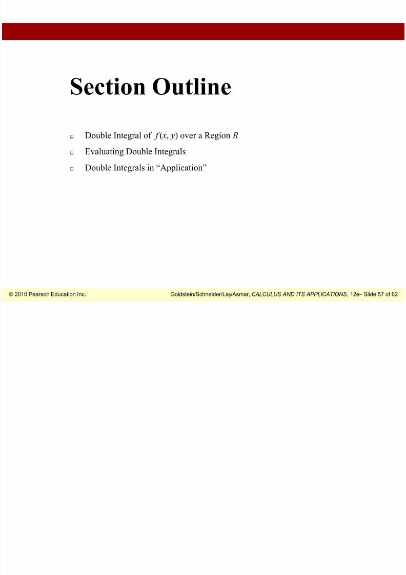
EXAMPLE

SOLUTION

Calculate the iterated integral.

Here g ( x) = x and h( x) = 2 x. We evaluate the inner integral first. The variablein this integral is y (because of the dy).

3

0

2

dx ydy x

x

2

2222

2

2

3

22

2

2 x

x x y ydy

x

x

x

x

Now we carry out the integration with respect to x.

2

270

2

13

2

1

2

1

2

3 33

3

0

33

0

2 xdx x

So the value of the iterated integral is 27/2.





Double Integrals in Application

EXAMPLE

SOLUTION

Calculate the volume over the following region R bounded above by the graphof f ( x, y) = x2 + y2.

R is the rectangle bounded by the lines x = 1, x = 3, y = 0, and y = 1.

The desired volume is given by the double integral . By the

result just cited, this double integral is equal to the iterated integral

R

dxdy y x 22

1

0

3

1

22 .dydx y x

We first evaluate the inner integral.

22223

23

3

1

23

3

1

22 23

26

3

1391

3

13

3

3

3 y y y y y xy

xdx y x




Double Integrals in Application

Now we carry out the integration with respect to y.

3

2800

3

2

3

260

3

20

3

261

3

21

3

26

3

2

3

262

3

26 33

1

0

31

0

2

y ydy y

CONTINUED

So the value of the iterated integral is 28/3.

Notice that we could have set up the initial double integral as follows.

This would have given us the same answer.

3

1

1

0

22 dxdy y x

Documents

1c. Functions of Several Variables_ppt_07