Embed Size (px)
Citation preview
University of WollongongResearch Online
University of Wollongong Thesis Collection University of Wollongong Thesis Collections
1998
Intelligent impact control in anti-personnel minedetectionAlireza Mohammad ShahriUniversity of Wollongong
Research Online is the open access institutional repository for theUniversity of Wollongong. For further information contact the UOWLibrary: [email protected]
Recommended CitationShahri, Alireza Mohammad, Intelligent impact control in anti-personnel mine detection, Doctor of Philosophy thesis, School ofElectrical, Computer and Telecommunications Engineering, University of Wollongong, 1998. http://ro.uow.edu.au/theses/1952


Intelligent Impact Control in Anti-Personnel Mine
Detection
A thesis submitted in fulfilment of the requirements for
the award of the degree
PhD
from
T TNIVERSITY
\ \ 70LLONGONG
By
Alireza Mohammad Shahri
B.Sc. Khajeh Nasir Toosi University, Tehran, Iran, 1985
M.E. (Hons) University of Wollongong, Wollongong, Australia, 1994
SCHOOL OF ELECTRICAL, COMPUTER AND TELECOMMUNICATIONS
ENGINEERING
August 1998

//
DECLARATION
This is to certify that the work presented in this thesis was carried out by the
author in the School of Electrical Computer and Telecommunications
Engineering at the University of Wollongong, and has not been submitted to any
other university or institute.
Alireza M o h a m m a d Shahri

///
To all victims of injustice
Thanks and love to those who sacrificed their life
and wealth to establish God rules on the earth.
Special thanks and love to Imam Hussein (AS) the
extraordinary teacher of freedom and martyrdom
who sacrificed his life and all his family to teach
how should resist against oppressors in the history.
Next, a warm thank to my wife, my son
Mohammaad, and my daughters Hosna and Zoha
who have supported and put up with me throughout
the course patiently.

IV
ACKNOWLEDGMENTS
In the name of God
Praise to God, the Cherisher and the Sustainer of the world. Without the
strengths and blessings from Him, I simply could not come to this stage.
However, whoever is not thankful to people is not thankful to God. Therefore,
some valuable contributions must be acknowledged here.
I would like to thank m y supervisor, Associate Professor Fazel Naghdy for his
invaluable guidance and supervision throughout this research work. In particular
I would like to thank him for his thorough review of m y thesis and published
papers.
I would also wish to thank m y friends Ali Yazdian, Ali Jalilian, Mohsen Kahani,
Peter Vial and Philip Ciufo for their valuable and helpful discussions. The
technical and adminishative supports of the departmental staff especially Carlo
Giusti, Joe Tisiano, Frank Mikk, Brian Webb, Steve Petrou, Tracy O'Keefe and
Maree Fryer are also acknowledged.
M y gratitude also goes to the Ministry of Culture and Higher Education ( M C H E )
of the Islamic Republic of Iran and the Department of Education, Employment
and Training (DEET) of Australia for their assistance with financial support and
postgraduate research scholarship (OPRS).

V
ABSTRACT
According to the International Committee of the Red Cross and Red Crescent
Societies (ICRC), there are approximately 110 million land-mines scattered
around the world in 64 countries. There are also as many mines in the stockpiles
around the world waiting to be deployed. As the result of explosions of mines,
around 2000 people are killed or maimed monthly. The victims are mostly
civilians including w o m e n and children who are trapped by mines after the end of
hostilities.
At present mine clearance mostly takes place manually. Unfortunately, on
average for every 5000 mines cleared one mine clearer is killed. Using the current
approach, it would take more than 1,100 years to clear the mines planted in the
world at a cost of US$33 billion.
The main focus of this thesis is to investigate the feasibility of developing a
robotic arm to detect buried Anti-Personnel (AP) mines in the field and hence to
overcome the above mentioned problems. The hand-prodding manual demining
procedure using a bayonet is simulated using a single degree force sensing
robotic arm.
The robotic device inserts a bayonet into the soil. A strategy to control the
bayonet is developed by modelling the dynamics of the manipulator and
environment, while adapting for variation in the stiffness sensed by the bayonet
when it comes in contact with the mine or any other object in the soil. A n explicit
impact control scheme is applied as the main control scheme, while three
different intelligent control methods are designed to deal with uncertainties and
varying parameters of the environment.

VI
A n analytical object recognition algorithm based on multiple prodding is
developed. A multi-probe mine detection mechanism with the ability to detect a
mine faster than a single-probe mechanism is also proposed.
All the developed algorithms are validated through computer simulation and
experimented work. The intelligent control algorithms have outperformed the
conventional controllers in all of the case studies. They have also produced
performances acceptable for demining operation.

VII
TABLE OF CONTENTS
DECLARATION II ACKNOWLEDGMENTS IV ABSTRACT V TABLE OF CONTENTS VE LIST OF FIGURES X LIST OF TABLES XIV
Chapter 1: Introduction 1 1.1. Introduction 2 1.2. Need for a Robotic Mine Detector 2 1.3. Problem Statement 3 1.4. Approach 4 1.5. Significance and Contribution of the Work 5 1.6. Thesis Aim and Objectives 6 1.7. Overview of Thesis 7 1.8. Publications Relating to Thesis 8
Chapter 2: Background 10 2.1. Introduction 11 2.2 Current Status of A P Land Mine Clearance Activities 11 2.3 A P Land Mine Detection Techniques 12 2.4. Automated Prodding Systems 16 2.5. A Review of Force/Impact Control Methods 27 2.6. Force/impact Control Methods 29 2.7 Summary 35
Chapter 3: Robot Arm and Environment Modelling 36 3.1. Introduction 37 3.2. Soil Dynamics 37 3.3. Dynamics of the Mine 40 3.4. Arm/Sensor model 42 3.4.1. Mathematical Modelling 43 3.4.2. Validation of the Model 55
3.5. A S M O D Modelling 57 3.5.1. Associative Memory Networks (AMN) 57 3.5.2. B-spline Basis Functions 60 3.5.3. One Dimensional B-Spline Model 62 3.5.4. Multi Dimensional B-spline Models 63 3.5.5. The A S M O D Model Presentation 64 3.5.6. A S M O D as a Neuro-Fuzzy Algorithm 67

VIII
3.5.7. A S M O D (Neuro-Fuzzy) Model Construction 70 3.5.8. A S M O D (Neuro-Fuzzy) Model Validation 72
3.6. Conclusion 75
Chapter 4: Design of Proposed Intelligent Impact Control Methods 76 4.1. Introduction 77
4.2. Impact Control 78 4.2.1. Impact Dynamics Model 78
4.2.2. Impact Control Guidelines 80
4.3. Neuro-Fuzzy Control 81 4.3.1. Direct Neuro-fuzzy Adaptive Control 82 4.3.2. Indirect Neuro-fuzzy Control 83
4.4. Design of Adaptive Indirect Neuro-Fuzzy Controller 85 4.4.1. Neuro-fuzzy Controller Design Based on the A S M O D Algorithm 88 4.4.2. Inverse A S M O D Model Construction 88
4.5. Intelligent Impact Control Design 89 4.5.1. Neuro-Fuzzy Adaptive Gain Impact Controller (NFAGC) 90 4.5.1.1. PI Velocity Control Design 90 4.5.1.2 Proportional Force Control Design 91 4.5.1.3. Simulation Scenario 94
4.5.2. Neuro-Fuzzy Impact Controller (NFIC) 97 4.5.2.1. Neuro-Fuzzy Inverse Model Construction 97 4.5.2.2. Feedforward NFIC without Velocity Controller 101 4.5.2.3. Feedforward NFIC with Velocity Controller 103
4.5.3. Neuro-Fuzzy Impact Control and PID Controller (NFIC/PDID) 105 4.5.3.1. P D Force Control Design 107 4.4.3.2. Simulation Results of the NFIC/PD Control Scheme 109 4.4.3.3. Simulation Results of the NFIC/PDPI Control Scheme 111
4.6. Conclusion 112
Chapter 5: Validation of Control Strategies 115 5.1. Introduction.... 116 5.2. Experimental Rig 116 5.2.1. D C Servo Motor Specifications 117 5.2.2. Load Cell Specifications 118 5.2.3. Linear Variable Differential Transformer (LVDT) 120 5.2.3.1. Operation of L V D T 121
5.2.4. Interface Circuits Description 123 5.3. Commissioning of the Experimental Rig 124
5.3.1. Hardware Problems 124 5.3.2. Software Problems 125 5.3.3. Implementation of Digital PID Controller 126
5.4. Validation ...127 5.4.1. Neruo-Fuzzy Adaptive Gain (NFAG) Controller 128
5.4.2. Neuro-Fuzzy Impact Controller (NFIC) 130 5.4.2.1. Feedforward NFIC with PI Velocity Controller 131

IX
5.4.2.2. Feedforward NFIC without Velocity Controller 133
5.4.3. NFIC/PID Results 136 5.4.3.1. Results of the NFIC/PD without Velocity Controller 136 5.4.3.2. Results of the NFIC/PDPI with Velocity Controller 138
5.5. Summary of Results 140 5.6. Conclusion.... 146
Chapter 6: Mine Detection Algorithm 148 6.1. Introduction 149
6.2. Land Mine Recognition Methods 149
6.3. Object Recognition Procedure 151 6.3.1. Feature Extraction of an Unknown Object 152
6.4. Estimation of the Object Radius and Centre Point 153 6.5. Mine Recognition Algorithm 157 6.6. Simulation 160 6.7. Experimental Results 163 6.8. Fuzzy Decision Making 166 6.9. Conclusion 172
Chapter 7: Conclusion and Further Research 173 7.1. Introduction 174
7.2. Summary of the Thesis 174 7.3. Future Research 176
References 178
Appendix A: Matcom Compiler 186 A.l. Introduction 186 A.2. Makefile for Building Standalone Executable Application 186
Appendix B: Algorithm in C++ Programming 188 B.l. Introduction 188 B.2. A Sample Code of the Intelligent Impact Controller 188 B.3. A Sample Code to build an A S M O D model 193
Appendix C: Plastic Cylindrical Anti-Personnel Mines 194

X
LIST OF FIGURES
Figure 2.1: A probe and two plastic A P land mines 12 Figure 2.2: Different methods of land mine detection 13 Figure 2.3: The lab. prototype deminer robot proposed by [Daw98] 17 Figure 2.4: The result of probing (b) and original image of three A P mines and a rock
(a) proposed by [Daw98] 18
Figure 2.5: Robot proposed by Anotoniae to detect buried mines [Ant95] 19 Figure 2.6: Pemex-B robot in grass and in packed 21 Figure 2.7: DETEC-1, the mobile and static unit [Gue97] 22 Figure 2.8: DETEC-2 [Gue97] 22 Figure 2.9: Close-up of probing mechanism [Ska96] 24 Figure 2.10: The prototype of automated prodding system and proposed terrain vehicle
to support the detection unit 25 Figure 2.11: Vehicle mounted mine detector ( V M M D ) [Ham96] 26 Figure 2.12: Explicit force controller block diagrams 28 Figure 2.13: Implicit force controller block diagrams 29 Figure 3.1: Result of dry beach sand (K=1.2 Kgf/m) 38 Figure 3.2: Result of wet beach sand (K=3.8 Kgf/m) 38 Figure 3.3: Result of river sand (2.6 Kgf/m) 39 Figure 3.4: Pottery clay (K =14 Kgf/m) 40 Figure 3.5: End-effector in contact with the environment 42 Figure 3.6: A/P cylindrical plastic mines (Picture Courtesy of Defence Science and
Technology Organisation) 42 Figure 3.7: Stiffness coefficients of the A/P cylinder plastic mine body and fuse (VS
50) 43 Figure 3.8: The dynamic model of the manipulator and end-effector in contact with the
environment 44 Figure 3.9: The open loop force model 47 Figure 3.10: A simple explicit force control with an inner velocity control loop 48
Figure 3.11: Step response and the root locus of the inner velocity loop using a PID controller 49
Figure 3.12: The root locus of the system with a PID velocity controller 50 Figure 3.13: Step response with the proportional force controller (Ke=14000, Kf=0.()25)
50 Figure 3.14: Velocity of the motor for the above step response 51 Figure 3.15: The step response corresponding to pair poles on the imaginary axis 53 Figure 3.16: Unit step response of the total system in 50 seconds. 53 Figure 3.17: The step response for Ke= 14() and Kt=().()25 54 Figure 3.18: Step response of the system with the designed PID controller contacting
the stiff environment (ke=28000 [Kgf/m]) 55 Figure 3.19: Root-locus of the system after removing poles on imaginary axis 55 Figure 3.20: Behaviour of the system using the designed compensator 57
Figure 3.21: Three-layer perceptron 59
Figure 3.22: B-spline type of an A M N s structure 60

XI
Figure 3.23: One-dimensional B-spline basis functions (degree 0, 1 and 2) for the Knot-Vector r\ = (1, 2, 3, 4, 5) 62
Figure 3.24: A two-dimensional B-spline basis functions with degree 1 and 2 in each dimension 63
Figure 3.25: The A S M O D algorithm structure for the example presented in Table 167 Figure 3.26: A typical triangular fuzzy membership function 68
Figure 3.27: Linguistic fuzzy output sets 70 Figure 3.28: A n Example of a Neuro-Fuzzy Model 72 Figure 3.29: Neuro-fuzzy adaptive gain control system 73 Figure 3.30: Open-loop position step response of the drive system 74 Figure 3.31: Simulation Results when stiffness is switching from 10 to 5000 75
Figure 4.1: Impact Dynamic Model 79 Figure 4.2: A general structure of a direct neuro-fuzzy adaptive controller 83 Figure 4.3: Structure of an indirect fuzzy adaptive control system. 84 Figure 4.4: A n online Feedforward Neural Network Model 85 Figure 4.5: Off-line inverse training mechanism 88 Figure 4.6: Neuro-fuzzy adaptive gain controller (NFAG) system 90 Figure 4.7: Step response of the inner velocity loop control 91 Figure 4.8: Gain-Varying Switch Non-linear System 92 Figure 4.9: A S M O D model to estimate the stiffness of the environment 93 Figure 4.10: Neuro-fuzzy adaptive gain controller (NFAG) system 94 Figure 4.11: S I M U L I N K graph of the N F A G control system 95 Figure 4.12: Environment model used in the simulation 95 Figure 4.13: Simulation results of N F A G and proportional force when stiffness changes
from 10 to 2500 [Kgf/m] 96 Figure 4.14: Simulation results of N F A G and proportional force when stiffness changes
from 10 to 5000 [Kgf/m] 96 Figure 4.15: Simulation results of N F A G and proportional force when stiffness changes
" from 10 to 7500 [Kgf/m] 97 Figure 4.16: Off-line inverse training mechanism 98 Figure 4.17: Graphical presentation of Sub-model No. 1 and No. 2 of the constructed
A S M O D model for NFIC controller 99 Figure 4.18: Graphical presentation of Sub-model No. 3 of the constructed A S M O D
model for NFIC controller 100 Figure 4.19: Validation of the constructed model for NFIC control 101
Figure 4.20: Block diagram of a NFIC method 102 Figure 4.21: Simulink graph for feed-forward NFIC 103 Figure 4.22: Simulation result of feedforward NFIC without velocity control loop when
stiffness switches from 10 to 5000 [Kgf/m] 103 Figure 4.23: Simulation result of feedforward NFIC without velocity control loop when
stiffness switches from 10 to 7500 [Kgf/m] 103 Figure 4.24: S I M U L I N K graph of the NFIC controller with PI velocity controller 104 Figure 4.25: Comparison of the simulation results with NFIC and without NFIC when
stiffness is switching from 10 to 2500 [Kgf/m] 104 Figure 4.26: Comparison of the simulation results with NFIC and without NFIC when
stiffness is switching from 10 to 5000 [Kgf/m] 105

xn Figure 4.27: Comparison of the simulation results with NFIC and without NFIC when
stiffness is switching from 10 to 7500 [Kgf/m] 105 Figure 4.28: NFIC controller block diagram 106
Figure 4.29: Root locus for the total system. 107 Figure 4.30: Step response of the PDPI explicit controller for the P D force controller
108 Figure 4.31: Step response of the PDPI explicit force controller 108 Figure 4.32: S I M U L I N K graph of the NFIC/PD control system 109 Figure 4.33: Simulation result of NFIC/PD when stiffness changes from 10 to 5000
[kgf/m] 110
Figure 4.34: Simulation result of NFIC/PD when stiffness changes from 10 to 7500 [kgf/m] 110
Figure 4.35: Simulation result of NFIC/PD when stiffness changes from 10 to 10000
[kgf/m] 110 Figure 4.36: S I M U L I N K graph of the NFIC/PDPI control system 111 Figure 4.37: Simulation result of NFIC/PDPI and PDPI when stiffness changes from 10
to 5000 [kgf/m] 112 Figure 4.38: Simulation result of NFIC/PDPI and PDPI when stiffness changes from 10 " to 7500 [kgf/m] 112
Figure 4.39: Simulation result of NFIC/PDPI and PDPI when stiffness changes from 10 to 10000 [kgf/m] 112
Figure 4.40: Force response comparison of all the proposed methods 114 Figure 5.1: End-effector connected to the force and L V D T sensor 117 Figure 5.2: Unbalanced mode Whetstone bridge 119 Figure 5.3: Cutaway view of the Schaevitz L V D T 121 Figure 5.4: Linear variable differential transformer 122 Figure 5.5: Experimental set up 123 Figure 5.6: Hardware configuration of deminer arm 124 Figure 5.7: Experimental result of N F A G Controller (A) 129 Figure 5.8: Experimental result of N F A G Controller (B) 129 Figure 5.9: Experimental result, of N F A G Controller (C ) 130 Figure 5.10: Experimental result of feedforward NFIC with PI velocity control loop (A)
131 Figure 5.11: Experimental result of feedforward NFIC with PI velocity control loop (B)
132
Figure 5.12: Experimental result of feedforward NFIC with PI velocity control loop (C ) 133
Figure 5.13: Experimental result of feedforward NFIC without velocity control loop (A) 134
Figure 5.14: Experimental result of feedforward NFIC without velocity control loop (B) 135
Figure 5.15: Experimental result of feedforward NFIC without velocity control loop (C ) 135
Figure 5.16: Experimental result of NFIC/PD controller (A) 137 Figure 5.17: Experimental result of NFIC/PD controller (B) 137 Figure 5.18: Experimental result of NFIC/PD controller (C ) 138 Figure 5.19: Experimental result of NFIC/PDPI controller (A) 139

XIII
Figure 5.20: Experimental result of NFIC/PDPI controller (B) 140 Figure 5.21: Experimental result of NFIC/PDPI controller (C ) 140
Figure 5.22: M a x i m u m overshoots of the force step response 143 Figure 5.23: Focus of the previous figure on NFIC/PDPI results 143 Figure 5.24: Comparison of the force range of different conventional and intelligent
methods 144
Figure 5.25: Comparison of the force range of different intelligent methods 144 Figure 5.26: Comparison of standard deviation of the force step response 145 Figure 5.27: Mode values for conventional and intelligent control methods 146
Figure 6.1: A buried anti-personnel mine beneath the soi 150 Figure 6.2: The three-probe robot in contact with a mine 151 Figure 6.3: Top view of the robot probes in contact with the cross section of a
cylindrical object 155 Figure 6.4: Side view of two contact points with a mine 156 Figure 6.5: A P mine recognition algorithm flow chart 159 Figure 6.6: Simulation based on different insertion points and different location for the
third c o ntac t p o i n ts 161 Figure 6.7: Simulation of A P mine recognition by multi-probe robot 162 Figure 6.8: Simulation of A P mine recognition by multi-probe robot 163 Figure 6.9: Objects which are used for experimental results 164 Figure 6.10: The Mamdani Fuzzy Inference System 167 Figure 6.11: Schematic diagram of fuzzy decision making 168 Figure 6.12: Inputs and output membership functions for F D M S 170 Figure 6.13: Outputs of the F D M S for eight objects 172

XIV
LIST OF TABLES
Table 4.1: A S M O D model construction for N F A G C 93 Table 4.2: A S M O D model construction for NFIC 99 Table 5.1: Hitachi D C servo motor specifications 117 Table 5.2: Load cell Specification 118 Table 5.3: Instrumentation amplifier specifications 120 Table 5.4: D C - L V D T specifications 123
Table 5.5: Performance of intelligent impact methods with PI velocity controller 141 Table 5.6: Statistical Comparison of the Intelligent Impact Control Methods 142 Table 6.1: Mine possibility table 153 Table 6.2: Experimental results for mine recognition algorithm 165 Table 6.3: Input and output variables of F D M S system and their characteristics 169 Table 6.4:: Rules of the fuzzy decision making 169 Table 6.5: Input and output data for F D M S 171

INTRODUCTION

Chapter 1 Introduction 2
1.1. Introduction
The main focus of this thesis is to investigate the feasibility of developing a
robotic arm to detect buried Anti-Personnel (AP) mines in the field. The need for
such a device and the problems associated with its development are initially
described in this chapter. The methodologies developed in this work to provide a
solution to some of the problems are then introduced. Finally the structure of the
thesis is presented and a summary of each chapter is given.
1.2. Need for a Robotic Mine Detector
According to the International Committee of the Red Cross and Red Crescent
Societies (ICRC), there are approximately 110 million land-mines scattered
around the world in 64 countries [Intl]. There are also as many mines in the
stockpiles around the world waiting to be deployed. As the result of explosions
of mines, around 2000 people are killed or maimed monthly. The victims are
mostly civilians including women and children who are trapped by mines after
the end of hostilities [Int2]. For every mine cleared, 20 are laid. In 1994, around
100,000 mines were cleared whereas 2 million new mines were planted. Overall,
anti-personnel mines are among the deadliest weapons used in the world today.
The United Nations Secretary-General has stated that "land-mines may be the
most widespread, lethal, and long-lasting form of pollution w e have yet
encountered" [Sta94].
At present mine clearance mostly takes place manually. Unfortunately, on
average, for every 5000 mines cleared, one mine clearer is killed. Using the
current approach, it would take more than 1,100 years to clear the mines planted
in the world at a cost of US$33 billion [Int2]. The hand-prodding technique is
the most reliable method of civilian mine clearance as it has a reliability of more

Chapter 1 Introduction 3
than 99.8%. A probe is manually insetted into the soil at a 30 degree angle,
approximately every five centimetres. W h e n an object is detected with higher
stiffness compared to the environment stiffness, more examinations are
conducted to identify the shape and size of the object. If the object is determined
to be a potential mine, a mine clearing team is called in to uncover or detonate the
object.
1.3. Problem Statement
In the work conducted in this thesis, the hand-prodding manual demining
procedure using a bayonet is simulated using a single degree force sensing
robotic arm. Four different stages can be identified in the task:
(a) The unconstrained and free motion of the arm towards the soil. At this
stage pure position control of the arm will be sufficient to maintain a stable
movement.
(b) Impact of the arm with the soil. At this stage, the arm encounters a rapid
change in the stiffness of the environment. Impact control is necessary to
prevent the oscillation of the arm, which may result in unstable behaviour of
the arm. Entry of the probe into the ground can be detected by a proximity
sensor.
(c) The movement of the arm in the soil. At this stage, the arm motion is under
physical constraints. In addition, there could be variations in the stiffness of
the environment as the arm comes in to contact with various objects in the
soil.
(d) Detection of an object in the soil and determining whether the object is a
mine. This requires various pattern recognition algorithms.

Chapter 1 Introduction 4
In this work an in depth study of the above phenomena is carried out. Various
methodologies are also inttoduced and developed to achieve a satisfactory
operation of the arm and a reliable detection of an A P mine.
1.4. Approach
The device inserts a bayonet into the soil. A suategy to control the bayonet is
developed by modelling the dynamics of the manipulator and environment, while
adapting for variation in the stiffness sensed by the bayonet when it comes into
contact with the mine or any other object in the soil. A n explicit impact control
scheme is applied as the main control scheme, while three different intelligent
control methods are designed to deal with uncertainties and varying parameters of
the environment.
Due to the nature of the task and the uncertainties associated with the model of
the system, the primary control methodology applied has been Intelligent Control
(IC). In the study carried out in this project, a neuro-fuzzy contioller is employed
to produce a compliant motion during impact control. Neural networks and fuzzy
systems are trainable dynamical systems which estimate the input-output
functions. Unlike statistical estimators, they estimate a function without a
mathematical model of how outputs depend on inputs. They are referred to as
model-free estimators [Kos92].
The approach adopted in this work is based on the class of (lattice-based)
Associative Memory Networks ( A M N s ) which have the abilities of universal
approximation and local generalisation. Examples of this class of networks
include the Radial Basis Function (RBF) network, the Cerebellar Model
Articulation Controller ( C M A C ) , the Basis (B)-spline network, Adaptive Spline
Modelling of Observation Data ( A S M O D ) and a certain class of fuzzy logic

Chapter 1 Introduction 5
network. The latter approach is selected as the main approach in this work to
implement the impact control.
Initially, a neuro-fuzzy adaptive gain controller (NFAGC) is designed to adapt
the force gain control according to the estimated environment stiffness. Then, a
feedforward impact controller (NFIC), which is based on the inverse dynamic
model of the aim in contact with the environment, is designed to control the
transient impact force if you move from free motion to constrained motion.
Finally the proposed NFIC, plus a conventional PID controller are employed to
switch from a PID controller to a neuro-fuzzy impact control (NFIC), when an
impact is detected. In this application, the characteristics of the environment
(soil) will change during the mine clearance operation. In other words, there is
uncertainty about the characteristics of the environment and its parameters.
One of the basic issues in intelligent control is to identify the model and the
variation of the system on-line. By introducing the ability of learning into the
control system, a plant becomes more flexible to deal with unpredictable and
complex, real-world environments. Learning, which is an integral part of any
intelligent control system, includes the heart of adaptive neural and fuzzy
modelling and control systems.
1.5. Significance and Contribution of the Work
The work carried out in this study is significant from different points of view. As
mentioned earlier, the A P mines currently cause a great deal of injury and death.
In addition, the current mine clearance methods employed are quite slow and
dangerous for the deminer. This work is a positive step towards the development
of a less dangerous and faster method of mine detection. Hence the project has
significant humanitarian values.

Chapter I Introduction 6
In addition, this work presents an in-depth study of intelligent control of a partly
structured environment. The methods developed for impact control and
constrained motion control of the mine detection arm are generic and can be
applied to similar situations in other applications.
Besides, all the introduced methods are validated through experimental work.
This highlights the effectiveness of the proposed methods in real time
applications.
1.6. Thesis Aim and Objectives
The primary aim of the project can be defined as developing appropriate
methodologies and techniques to mimic the hand-prodding manual demining
procedure using a single degree force sensing robotic arm. This aim has been
pursued by achieving the following objectives:
• A n in depth critical study of the previous work in this area.
• Modelling of the robotic arm and its environment using both mathematical and
intelligent methods.
• Design and development of intelligent impact controllers using neuro-fuzzy
methods.
• Design and development of mine detection algorithms.
• Validation of the developed methods using both computer simulation and
experimental work.
Chapter I Introduction 7 _
1.7. Overview of Thesis
The work carried out is presented in this thesis through seven chapters. The
problem statement, aim and objectives of the work, and a brief introduction to the
A P mine detection arm and major control schemes developed in the work are
provided in Chapter 1. The results of the literature search of the previous work in
the two areas of automatic mine detection and force control techniques is set in
Chapter 2. Chapter 3 is dedicated to the modelling of the robot arm, sensors and
environment. A mathematical model and a neuro-fuzzy model of the robot arm
in contact with the environment are developed and their performance is
compared. The advantages of the neuro-fuzzy model over the mathematical
model is also demonstrated in this chapter through computer simulation.
The intelligent impact control is studied in Chapter 4. An in depth analysis of
impact and the methods employed for its control are presented. Three neuro-
fuzzy impact control techniques developed in this work are then explained and
validated through computer simulation.
Chapter 5 presents the experimental rig used in the project and the experimental
work carried out to validate the impact control methods. In this chapter, the
software and hardware problems encountered in developing the experimental rig
are also described.
The mine detection algorithm developed in the work is described in Chapter 6.
A n analytical object recognition algorithm based on multiple prodding is
presented. A multi-probe mine detection mechanism with the ability to detect an
A P mine faster than a single-probe mechanism is also proposed. The proposed
algorithm is validated through computer simulation and experimental work.

Chapter I Introduction 8
A summary of the work conducted in this project, its outcomes and future work
to enhance the performance of the A P mine detector robot arm are provided in
Chapter 7. This chapter also provides the conclusions reached at in this work.
1.8. Publications Relating to Thesis
A. M. Shahri, F. Naghdy, "Neuro-Fuzzy Adaptive Torque Control of a SCARA
Robot", Proceedings qf the Australian New Zealand Conference on Intelligent
Information Systems (ANZIIS 96), IEEE 96TH8234, pp. 241-244, Adelaide,
South Australia, 18-20 November 1996.
A. M . Shahri, F. Naghdy, "Adaptive Neuro-Fuzzy Compliance Control with the
Ability of Learning", Proceedings of International Conference on Intelligent and
Cognitive Systems (ICICS-96), pp. 74-79, Tehran, Iran, September 23-26, 1996.
A. M . Shahri, F. Naghdy, "Intelligent Compliance Control in Anti-Personnel
Mine Detection", Proceedings of Fourth Annual Conference on Mechatronics
and Machine Vision in Practice (M2vip97), IEEE Computer Society, pp. 84-91,
Toowoomba, Australia, September 23-25 1997.
A. M . Shahri, F. Naghdy, P. Nguyen, "Neuro-Fuzzy Compliance Conttol with the
Ability of Skill Acquisition from Human Experts", Proceedings of First
International Conference on Conventional and Knowledge-Based Engineering
Systems (KES'97), pp. 442-448, Vol 2, IEEE 97TH8250, Adelaide, Australia,
May 21-23 1997.
A. M . Shahri, F. Naghdy, "Anti_Personnel Mine Detection Manipulator",
Proceedings qf the International Conference on Field and Service Robotics
(FSR'97), Australian Robot Association INC., Canberra, Australia 8-10
December 1997.
Chapter 1 Introduction 9
A. M . Shahri, F. Naghdy, "Mechatronics Approach to Detect Anti-Personnel
Mines", Proceedings qf the International Conference "Detection and
Remediation Technologies for Mines and Minelike Targets III", (SPIE'98), pp.
808-819, 13-17 April, 1998.
A. M . Shahri, F. Naghdy, "Anti-Personnel Mine Detection Algorithm Based on a
Multi-Probe Robotics Arm", To be published in Conference Proceedings oflARP
Workshop on Robotics for Humanitarian Demining, Toulouse, France, 14-15
September, 1998.
A. M . Shahri, F. Naghdy, "Neuro-Fuzzy Impact Control (NFIC) for Anti-
Personnel (AP) Mines Detection", To be published in Conference Proceedings qf
the Fifth International Conference on Control, Automation, Robotics and Vision
(ICARCV98), Singapore, 8-11 December, 1998.
Talaie, Afshad. Shahri, Alireza M. Talaie, Farhad, "Adaptive Spline Modelling of
Observation Data ( A S M O D ) : A Solution to the Problems in Conducting
Polymer-based Sensors", Journal of Synthetic Metals, p 63-67, v 79 n 1 Apr 30
1996.
A. M . Shahri, F. Naghdy, "Anti_Personnel Mine Detection Manipulator", in
"Field & Service Robotics" Springer-Verlag, ISBN: 185230392, July 1998.
A. M . Shahri, F. Naghdy, "Neuro-Fuzzy Compliance Control of Peg-in-Hole
Insertion", Submitted to International Journal of Robotics & Automation (IJRA).

BACKGROUND

Chapter 2 Background }j
2.1. Introduction
In this chapter two distinct reviews of different Anti-Personnel (AP) land mine
detection techniques and different force control strategies will be presented. The
first review will outline research directions currently pursued being in this area
and will highlight the contribution of the work conducted in this thesis. Five
major research works will be reviewed. These works cover the two major
approaches to mine detection: contact and non-contact sensing techniques.
As part of the second review, a review of previous force/impact control research
will be presented in Section 2.5. Then some of the new impact control methods
are discussed. Finally, a summary of this chapter is presented.
2.2 Current Status of AP Land Mine Clearance Activities
Currently, metal detectors are mostly employed as a first step in the demining
process. Metal detectors work by measuring the disturbance of an emitted
electromagnetic field caused by the presence of metallic objects in the soil
[Tsi96]. The hand-prodding technique which is one of the most reliable methods
of mine clearance, is used as the second step to locate the A P mines. A probe is
manually inserted into the soil at a 30 degree angle, approximately every five
centimetres. Figure 2.1: shows a probe and two plastic A P land mines.

Chapter 2 Background J2
_F-__ll
Figure 2.1: A probe and two plastic A P land mines
When an object with higher stiffness compared to the stiffness of the
environment is detected, more examinations are conducted to identify the shape
and size of the object. If the object is determined to be a potential mine, a mine
clearing team is called to uncover or detonate the object as the third and last step
of the demining procedure. The problem associated with this method is that A P
mines are intentionally fabricated with almost no metal parts, except for the
striker pin. Although, it is possible to increase the sensitivity of the metal
detectors to detect very tiny items (a tenth of a gram of metal at a depth of 10
cm), this will considerably increase the rate of the false alarms and therefore lead
to the detection of unwanted small debris and artefacts.
There is a considerable difference between military and humanitarian mine
clearance procedures. In the former case the aim is to make a quick breach in the
minefield usually with a success rate of around 80%, while in the latter approach
the demining process is expected to have a higher success rate of above 99.6%
[Nic96].
2.3 AP Land Mine Detection Techniques
The work carried out so far on A P mine detectors has centred on their sensory
aspects. Very few research groups have attempted to develop a specific mobile

Chapter 2 Background 13
robot to automatically manoeuvre the sensory device on the mine field. The non-
contact sensing techniques have a success rate of up to 9 0 % , which is accurate
enough for military applications but not for civil demining. It should be also
pointed that a mine detected by the non-contact sensing methods ultimately will
be located and cleared by employing a contact sensing technique such as manual
prodding.
The two major categories of mine detection approaches and various techniques
employed in each approach are illustrated in the chart shown in Figure 2.2. The
chart also highlights the specific characteristics of each method including the type
of the sensor, the stage of the development or the maturity of the technique, its
advantages, disadvantages, and cost/complexity.
Sensor
Maturity
Advantage
Mcadvant-gc
Cost
Human Fuiger
Available
Accurate
Reliable
Slow Dangerous
Low ^ J
Forte / Tactile
Near
Accurate
Reliable
Fast
Not Flexible
Medium
Induction Coil
Available
Very Common
Slow Inaccurate
Dangerous
Low
^DogNose ^ Odor Sensor Available
Good for Area Detection
Inaccurate Locating
Nodding is need
Medium
Antenna
Far
Fast
Complex
Heavy-Weight
High j
Infrared Senost
Near
Fast
Soil Dependant
Medium
Combination
Near
Depends on
Serauis "»"l
Complex
Medium/High V _ _ _ J
Figure 2.2: Different methods of land mine detection
2.3.1 Non-Contact Sensing Techniques
The current non-contact sensing methods tested in both laboratories and
landmine fields are:
• Conventional and Advanced Metal Detectors (Impulse M D ) • Infra-Red Sensors (IR)

Chapter 2 Background 14
• Ground Penetrating Radar (GPR)
• Dogs, e.g. Mechem Explosive and Drug Detection Systems(MEDDS)
• Elecuonic Dog's Nose
• Micro Electro Mechanical Systems ( M E M S )
• Bio-Sensors
• Millimetre Wave Radar ( M W R )
• Nuclear Methods and Nuclear Magnetic or Quadruple Resonance ( N M R / N Q R )
• Thermal Neutron Activation (TNA).
In the work conducted by Fritzche and Trinkhaus [Fri95], ground penetrating
radar (GPR) sensors and high sensitivity metal detectors have been used to
identify metal mines. The aim has been to eventually employ the two sensors in
parallel and to fuse the data produced by them to provide a more robust and
reliable detection process. G P R seems to be one of the few technologies feasible
for detection of anti-tank and anti-personnel mines. There is, however, a great
deal of work required to accommodate the technology in an appropriate field
device [Fri95]. The F O A team in Sweden has started a project in this area using
a 0.3-3 G H z G P R system [Chi95]. The Lawrence Livermore National Laboratory
(LLNL) has also developed and patented a new technology, the Micropower
Impulse Radar (MIR) [Bru94].
According to the information available on the World Wide W e b [Aze95], the U S
Army Research has provided funding for Duke University together with five
other institutions, including Caltech, Georgia Tech, Ohio State University and
Stanford University, to explore innovations in mine detection, ranging from a
microelectronic chemical-sniffing "nose", through-the-air ultrasound, to ground-
shaking seismic waves.
In a recent survey conducted by C. Bruschini and B. Gros from Demining
Technology Centre (DeTec), most of the current sensor technologies have been
studied in detail [Bru97]. Although all of these approaches have the capability to

Chapter 2 Background 15
detect A P mines, they generally suffer from various limitations and drawbacks,
which include sensitivity to weather/soil conditions, mine depth, poor
performance in heavy vegetation and wet soil, and by being not applicable in all
conditions. In order to overcome these limitations, researchers [Gue97] and
[Mcm96] are working on fusion techniques to fuse different data obtained from
multiple sensors to provide a more reliable mine detection device, with
considerably less false alarms.
In another critical review James Trevelyan [Tre97] has tried to be more realistic
and study more practical and real problems involved in mine detection methods.
He has particularly addressed the robotics researchers to learn from the land mine
problems and redirect their research toward more practical and worthy
approaches. According to his argument, robots have been tried at great expense,
but without success. H e also suggested that a robot arm was not an appropriate
solution for mine clearance. Research should preferably be directed towards
improving simple and low-cost robotics devices which can provide some useful
improvements in safety and cost-effectiveness.
According to Trevelyan [Tre97] the Pemex-B deminer robot proposed by Nicoud
[Nic95a] lacks a reliable mine detection sensor and the robot proposed by British
company E R A [Dan97], consisting of a robot arm and ground peneuating radar,
is not an appropriate device. He has also criticised all the armoured vehicles
which are claimed to withstand the effect of A P mines as they would set off the
mines by ground pressure or tripwires. All the work earned out on the
automation of the probing process by different research groups, such as Kenneth
Dawson-Howe [Daw97a] and [Daw97b] are blamed for having a non-realistic
assessment of the cost effectiveness of such robots, or do not address the practical

Chapter 2 Background 16
difficulties of dealing with stones, rubbish, roots and other extraneous objects
encountered in real minefields.
2.3.2 Contact Sensing Techniques
Manual prodding and automated prodding are the main techniques pursued in this
category. While some destructive techniques such as mobile mechanical
approaches could have been included, though have not been. In the destructive
methods, very heavy mobile mechanical systems are used to set off the A P mines.
Such an approach is only acceptable in military mine clearance applications not
in civilian mine clearance. As the focus of this research is on civilian mine
clearance, the destructive mechanical approaches are not addressed.
2.4. Automated Prodding Systems
Since all the automated prodding systems imitate manual prodding, they have
many common features. The most important feature of these systems is their
light weight to avoid accidental explosion of the mine if they move over them.
Since these systems are mainly used in underdeveloped parts of the world with
little high technical expertise and knowledge, they should be simple and easy to
maintain and operate. Cost efficiency is another critical issue which should be
considered likewise. There are a few research groups trying to design and
implement semi/full autonomous prodding systems to detect and locate A P
mines. These systems are also still in the laboratory condition test stages. Field
trials are essential to validate the performance and robustness of such devices.
2.4.1 Probot: Autonomous Probing Robot
This research is conducted in the Computer Vision and Robotics Research Group
of the Department of Computer Science at Trinity College Dublin. In this work a
robotics solution to the problem of automatic detection of APLs is proposed.

Chapter 2 Background 17
This solution is based on the physical detection of A P mines using a sharpened
probe in a fashion similar to that employed by human deminers. As the probe is
inserted into the ground (at 30 degrees relative to the horizon in order to avoid
triggering the landmine) the axial force applied to the probe is sensed. The force
information, together with absolute position information, is used to determine the
presence of buried objects [Daw97a]. Figure 2.3 illustrates the implemented
demonstrator system which is capable of scanning and inserting the probe into the
soil in order to locate unknown objects under the ground. The system [Daw98]
can accommodate an array of independent probes and a combination of other
sensors, such as a Metal Detector ( M D ) and Ground Penetrating Radar (GPR) to
speed up the probing task and increase the accuracy of the system.
Figure 2.3: The lab. prototype deminer robot proposed by [Daw98]
The system consists of an X Y table to allow probing over a limited test area. A n
electrical linear actuator drives the probe attached to a force sensor to sense
resistance to the probe. The system provides force and position (from an optical
encoder) data to control the probing task not to exceed a pre-selected threshold
(15 Newtons) and record the depth of insertion. The work conducted on the force
control of the probe does not seem to be considerable. In addition, it is assumed
Chapter 2 Background jg
that the leading edge of an object is probed in order to minimise the risk of
triggering the mine by probing it on the top surface. However, the proposed
object recognition algorithm is based on the data obtained from probing on the
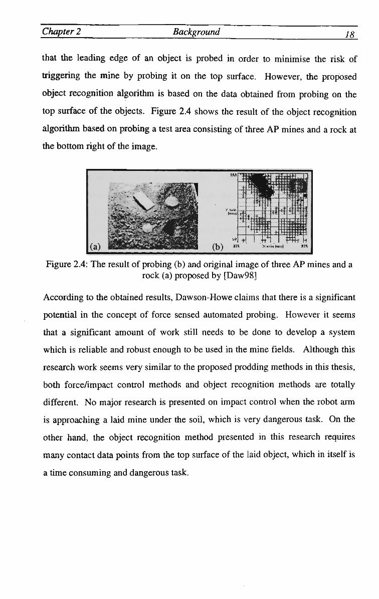
top surface of the objects. Figure 2.4 shows the result of the object recognition
algorithm based on probing a test area consisting of three A P mines and a rock at
the bottom right of the image.
Figure 2.4: The result of probing (b) and original image of three A P mines and a rock (a) proposed by [Daw98]
According to the obtained results, Dawson-Howe claims that there is a significant
potential in the concept of force sensed automated probing. However it seems
that a significant amount of work still needs to be done to develop a system
which is reliable and robust enough to be used in the mine fields. Although this
research work seems very similar to the proposed prodding methods in this thesis,
both force/impact control methods and object recognition methods are totally
different. N o major research is presented on impact control when the robot arm
is approaching a laid mine under the soil, which is very dangerous task. O n the
other hand, the object recognition method presented in this research requires
many contact data points from the top surface of the laid object, which in itself is
a time consuming and dangerous task.

Chapter 2 Background jg
2.4.2 Ground Probing Sensor for Automated Mine Detection
In Zagreb, Croatia, D. Anotoniae [Ant95] from the Faculty of Electrical
Engineering and Computing, Department of Control and Computer Engineering
in Automation, Ministry of Interior, has studied the development of a semi-
autonomous ground probing land-mine detection system. The concept resembles
the process of manual probing by using a teleoperated mobile robot equipped
with an appropriate ground probing sensor. The work so far has focused on the
development of a force detection sensor. The available information neither
reveals the nature of the detection algorithm nor any experimental results on the
performance of the device. The system consists of one linear servomechanism
attached to a 30 cm long needle. Force and position data are used to detect the
depth of a buried object. Anotoniae [Ant95] has proposed a method to determine
the contour of the buried object by analysing the collected data from probing
every 2.5 cm. According to this method, it is necessary to use more probing
around the point where an obstacle is detected. Figure 2.5 illustrates the
proposed semi-automated probing system remotely controlled by a human
operator.
Figure 2.5: Robot proposed by Anotoniae to detect buried mines [Ant95]
In Figure 2.5, two robotics arms are shown whereas the research has only focused
on the arm needed to detect the buried mine. Detection of the touch point is
Chapter 2 Background 20
performed by the force profile analysis. As there is no force measured before
touching the ground, contact with the surface of the soil builds up an increasing
force profile proportional to the depth of the insertion. According to Anotoniae,
the acting force should be below the activating force triggering the mine fuse
which is as low as 10 N for A P landmines. However, how this significant goal is
achieved is not clarified. The object recognition algorithm presented by
Anotoniae, interprets the collected data by converting it to a 256 level grey scale
image. According to this algorithm, the maximum sensing depth corresponds to
white and the sensor reference level is black. A proper threshold level
adjustment is used to enhance the quality of the image. Another algorithm wire
model is presented in this work which is claimed to have the advantage of
exuacting the information of exact position and depth of a buried object. Finally,
Anotoniae has concluded that the proposed system is designed to fill a gap
between the accurate but slow and hazardous manual probing technique, and
various non-contact sensing methods with insufficient accuracy for civil
demining.
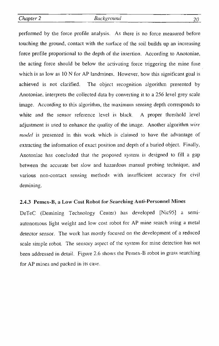
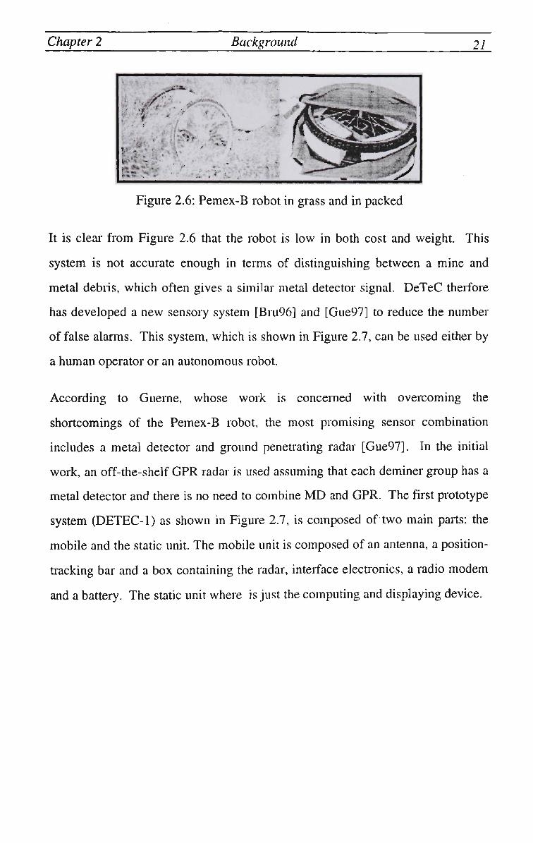
2.4.3 Pemex-B, a Low Cost Robot for Searching Anti-Personnel Mines
DeTeC (Demining Technology Center) has developed [Nic95] a semi-
autonomous light weight and low cost robot for A P mine search using a metal
detector sensor. The work has mostly focused on the development of a reduced
scale simple robot. The sensory aspect of the system for mine detection has not
been addressed in detail. Figure 2.6 shows the Pemex-B robot in grass searching
for A P mines and packed in its case.
Chapter 2 Background 21
-_--'-**• *
~ ''/ft-' • ' ??•
. - r'< [ S ^
ft**":'-
• • ? \
f ' *••,
\„ .
' • ^ • ' ; . ,
.., f*l£**"
'= fs^HfaS ' "llf >____ ^^^IM
MJ ;>*_
S N. i ,r_Jfln
* ^
"'^
Figure 2.6: Pemex-B robot in grass and in packed
It is clear from Figure 2.6 that the robot is low in both cost and weight. This
system is not accurate enough in terms of distinguishing between a mine and
metal debris, which often gives a similar metal detector signal. DeTeC therfore
has developed a new sensory system [Bru96] and [Gue97] to reduce the number
of false alarms. This system, which is shown in Figure 2.7, can be used either by
a human operator or an autonomous robot.
According to Guerne, whose work is concerned with overcoming the
shortcomings of the Pemex-B robot, the most promising sensor combination
includes a metal detector and ground penetrating radar [Gue97]. In the initial
work, an off-the-shelf G P R radar is used assuming that each deminer group has a
metal detector and there is no need to combine M D and GPR. The first prototype
system (DETEC-1) as shown in Figure 2.7, is composed of two main parts: the
mobile and the static unit. The mobile unit is composed of an antenna, a position-
tracking bar and a box containing the radar, interface electronics, a radio modem
and a battery. The static unit where is just the computing and displaying device.

Chapter 2 Background 22
Figure 2.7: DETEC-1, the mobile and static unit [Gue97]
The concept of using two units has proved to be one of the drawbacks of this
system. It is hard for a deminer to trust the decision taken by someone at a safe
distance based on the information received from the static unit. Deminers prefer
to see the data and analyse it themselves rather than someone else far from the
minefield to do it for them. To overcome this problem, DETEC-2 as shown in
Figure 2.8, is integrated in one unit. The major modification in this prototype is
that the G P R antenna to scan the mine field is not carried by hand any more. It is
clear from Figure 2.8 that the G P R antenna has now been located on the top of
the system. The antenna is capable of scanning the front area from left to right
angular motion and back to forward linear motion.
Figure 2.8: DETEC-2 [Gue97]

Chapter 2 Background 23
More details can be found in [Bro98] which reports some results of the DETEC-2
being tested on a real mine field in Cambodia.
2.4.4 A Mechanical Means of Land Mine Detection
This work was initially started as a landmine project for a group of mechanical
students at the University of Alberta, supported by the Defence Research
Establishment Suffield (DRES). Initially a list of minimum design requirements
was given to the students. The best research proposal satisfying the requirements
was then chosen for further work. The final design consisted of an automated,
multiple-prodding device designed to be mounted on the front of a remotely
controlled all terrain vehicle (ARGO).
The detection unit consisted of two sets of probes for Anti-Personnel and Anti-
Tank (AT) mines mounted by springs to sliders attached to the connecting rods.
A slider-crank mechanism is used to move the probes. A motor on the rack
drives two parallel crankshafts, one for the A P probes and the other for the A T
probes. Figure 2.9 shows a close-up of the probes and the crank shaft assembly.
The connecting rods convert the motion of the crank shafts into a reciprocating
motion on the probes.

Chapter 2 Background 24
Figure 2.9: Close-up of probing mechanism [Ska96]
At the back of each probe is an accelerometer, which measures the vibration from
the probe as it strikes an object. The amplitude and frequency of the vibration
signals change according to the object in contact with the probes.
The work has successfully completed the consti-uction of a test stand system,
including a pneumatic driver system, data acquisition and control system.
According to the project report, an automated signal processing and analysis
procedure has also been developed to recognise the unknown buried objects. N o
report is available on the success of the signal processing and other aspects of the
device.
The D R E S implemented test system [Ska96], consists of two pneumatic
cylinders, a steel frame to provide support and adapt for evaluation of different
operating conditions and various instrumentation. The insuumentation includes
an accelerometer, two pressure uansducers, an L V D T , and a rotary
potentiometer. The prodder system is actuated by two pneumatic cylinders to
Chapter 2 Background 25
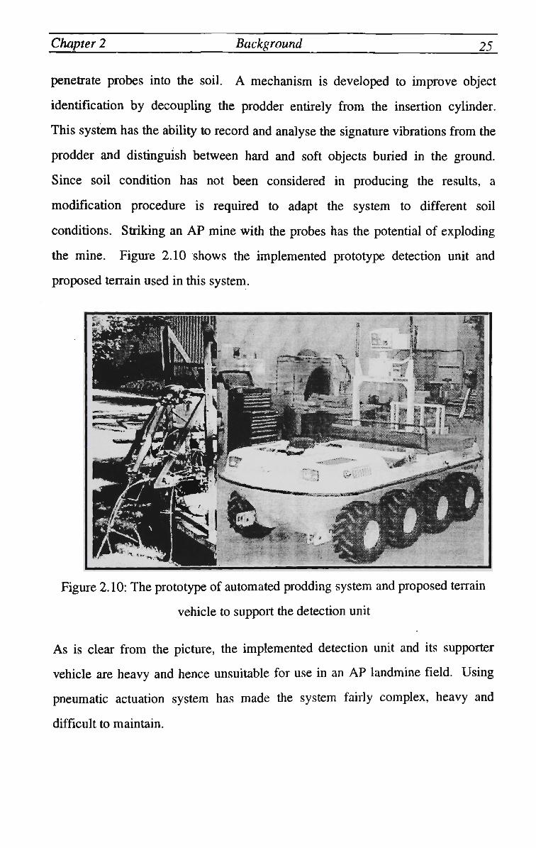
penetrate probes into the soil. A mechanism is developed to improve object
identification by decoupling the prodder entirely from the insertion cylinder.
This system has the ability to record and analyse the signature vibrations from the
prodder and distinguish between hard and soft objects buried in the ground.
Since soil condition has not been considered in producing the results, a
modification procedure is required to adapt the system to different soil
conditions. Striking an A P mine with the probes has the potential of exploding
the mine. Figure 2.10 shows the implemented prototype detection unit and
proposed terrain used in this system.
Figure 2.10: The prototype of automated prodding system and proposed terrain
vehicle to support the detection unit
As is clear from the picture, the implemented detection unit and its supporter
vehicle are heavy and hence unsuitable for use in an A P landmine field. Using
pneumatic actuation system has made the system fairly complex, heavy and
difficult to maintain.
Chapter 2 Background 26
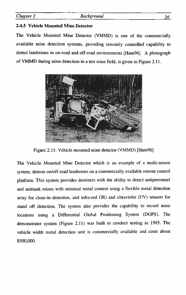
2.4.5 Vehicle Mounted Mine Detector
The Vehicle Mounted Mine Detector ( V M M D ) is one of the commercially
available mine detection systems, providing remotely controlled capability to
detect landmines in on-road and off-road environments [Ham96]. A photograph
of V M M D during mine detection in a test mine field, is given in Figure 2.11.
Figure 2.11: Vehicle mounted mine detector ( V M M D ) [Ham96]
The Vehicle Mounted Mine Detector which is an example of a multi-sensor
system, detects on/off-road landmines on a commercially available remote control
platform. This system provides deminers with the ability to detect antipersonnel
and antitank mines with minimal metal content using a flexible metal detection
array for close-in detection, and infra-red (IR) and ultraviolet (UV) sensors for
stand off detection. The system also provides the capability to record mine
locations using a Differential Global Positioning System (DGPS). The
demonstrator system (Figure 2.11) was built to conduct testing in 1995. The
vehicle width metal detection unit is commercially available and costs about
$500,000.

Chapter 2 Background 27_
2.5. A Review of Force/Impact Control Methods
Industrial robots have a wide variety of applications in industry. Most of the
robots require control of position in some Cartesian degree of freedom and
control of force in others. Apart from some exceptions such as application of
robots in paint spray or visual servoing, the majority of the robotics applications
require interaction with the environment. Position controlled manipulators are
ideal for tasks, such as pick and place or spot welding with no interaction or
minor interaction with the environment. However in these applications a very
small position error, while the arm is in contact with the stiff environment, can
cause a large reaction forces exerted on the arm. There are other robotics
applications, such as pushing, polishing, assembly, scrapping, grinding, and
twisting in which force control is a vital requirement. In these types of tasks,
there should be at least one degree of freedom force controlled link in addition to
the position control of other links.
Impact phenomena plays an important role in the field of robotics particularly
when the robot is in contact with the environment. The transition between the
conditions of free motion and constrained motion which induces an undesirable
reaction force, is called impact phenomenon. The most common assumption
made in the control of a robotic manipulator is that the robot is either moving in a
free space or is constrained by a known environment.
Robot manipulators and drive systems can experience instability or poor control
performance after collision with a surface. Similarly, during mechanical mine
detection process, an impact force is generated which may cause the robot to
oscillate and hence lose its contact with the environment. This usually results in
an oscillatory motion of the robot as the stiffness of the environment suddenly

Chapter 2 Background 28
changes while the gain of the control system remains constant. This oscillation
can set off an A P mine.
Therefore, force/impact conttol is a vital requirement for a robot under
constrained motion. The control methods used in the constrained motion tasks
can be categorised into passive compliance and active compliance methods. In
this thesis, the active compliance is discussed in details. Active control force
methods can be also categorised into hybrid position/force control and impedance
control.
Hybrid position/force control can be classified into explicit or force-based and
implicit or position-based control methods depending on the method by which
force information is included in the forward control path [Vuk94]. Position-
mode and force-mode are the main two categories of the impedance control
methods. In explicit force conttol [Rai81][Wed88], the reference command is
force whereas in implicit force control [And88] it is position. This implies that
the primary feedback signal in explicit force control scheme is force, while in
implicit control is position. Figures 2.12 and 2.13 show general block diagrams
of explicit and implicit force control schemes.
^Q-Explicit Force Controller
Robots Manipulator
m >
Figure 2.12: Explicit force controller block diagrams

Chapter 2 Background 29
?Q-Implicit Force
Controller
x c
•7TT Position Controller
Robots
Manipulator
X F mm »
Figure 2.13: Implicit force controller block diagrams
There are different control strategies proposed by different researchers for
explicit force-based control, such as simple proportional control to different
subsets of the PID controllers (i.e. I, PI, PD, PID). A n extensive review and
analysis of all these strategies can be found in [Vol91].
2.6. Force/impact Control Methods
There are a number of different force control methods reported in the literature to
control a manipulator coming in contact with a stiff environment. They include;
active stiffness control [SaI80], maximal active damping [kha86], passive
compliance and damping [Xu88], integral explicit force control [Tou89],
impedance control and proportional explicit force control [Hog85a].
Volpe and Khosla identified three phases in controlling a robot approaching a
stiff environment: free motion, impact transience, and force control [Vol91].
Mandal and Payandeh proposed an approach based on the same idea of three
phase but their emphasis was on experimental result and implementing the impact
control strategies [Man93]. Their results indicate that for very stiff environment,
stable impact control may be achieved at low velocities only, and that for a
compliant system, there is a trade off between approach velocity, compliance,
sampling time and the bandwidth of the robot system.

Chapter 2 Background 30
Tornambe has carried out extensive analytical modelling for one-degree-of-
freedom impact between two bodies [Tor96]. H e proposed a control scheme on
the basis of an observer that is able to asymptotically estimate the impact induced
forces and to allow their asymptotic compensation when the two bodies are in
contact. The proposed control scheme is just supported by a simulation test
which is far from a physical system, particularly in a system with force sensing.
W u and his colleagues proposed a solution to the robust impact control and force
regulation by adding a positive acceleration feedback to the feedback loop
[Wu96]. A switching control suategy is also designed to guarantee the stability
of the impact control. This approach is implemented and the results are compared
with the impedance and hybrid force/position control. Results demonstrates the
advantages of the proposed impact control scheme over the other methods. A
stochastic optimal control approach capable of modelling uncertainties in contact
environment, force sensing, and manipulator dynamics is proposed by Lee and
Chiu [Suk96]. Simulation results have verified that the stochastic optimal control
approach yields a controller optimally robust in terms of performance according
to the statistics of the uncertainties. Walker utilised kinematic redundancy of
robot manipulators to find configurations that minimised the effect of impact at
similar approach velocities [Wal94]. Model predictive control (MPC) proposed
by Carufel and Necsulescu is another impact control scheme which allows for the
control in both conditions, free and contact, without having to deal with
switching control law [Car95]. However it is claimed that M P C can solve the
impact-contact motion control problem, though no real-time implementation is
reported.
Increasingly, new impact control schemes combined with conventional force
control methods are proposed as solutions to the problem of impact control. A

Chapter 2 Background 31
few recent impact control schemes proposed by researchers are discussed in more
details in the following sections.
2.6.1. Impact Control Using Force and Vision Feedback
Since transition from non-contact to contact states should be fast and stable, a
new method using vision feedback in addition to the force feedback is proposed
by Nelson and his colleagues in the Robotics Institute at the Carnegie Mellon
University [Nel95]. In this method both vision and force feedback signals are
considered simultaneously in the connol strategy until the camera lens system is
unable to accurately resolve the location of the end-effector relative to the contact
surface. At this stage the conhol system switches to pure force control. The use
of visual servoing has simplified the force control problem by allowing a low
gain force control while approaching a rigid surface with a high velocity, hence
minimising the impact force and avoiding bounce between the surfaces.
The force conuol portion of the vision/force servoing strategy is based on a
combination of hybrid force/position conhol [Rai81] and damping force control
[Whi85]. The aim of visual servoing is to overcome the problem associated with
guarded motion and pure force conhol strategies upon impact. During a guarded
motion, the surface is approached under position control while the force sensor is
monitored. If the measured force exceeds a threshold, motion is immediately
stopped and a force control strategy is invoked. In visual servoing, when the end-
effector is far from the environment, the end effector is driven at a high speed.
The velocity, however, starts to decrease as the end effector comes closer to the
surface. Hence a low gain force conuoller can achieve a stable uansition to
contact state.
The introduction of visual servoing is quite expensive and requires extensive
computing power to handle real time image processing and control. It, however,

Chapter 2 Background 32
improves the manipulator performance during contact transitions. This approach
is not a feasible solution for the mine detection task.
2.6.2. Jump Impact Control (JIC)
The jump impact control method proposed by Chiu and Sukhan [Chi97] is
derived from stochastic optimal control theory and jump linear system theory
with the goal of creating an impact/force controller which is robust to the
environment dynamics and collision surface location uncertainties. Chiu justifies
the use of word 'jump' in JIC method, because after a collision there is a jump in
the system dynamics. The 'jump' implies that the state space description of the
system dynamics changes abruptly. The manipulator collision dynamics in the
presence of uncertainties can be constructed within the framework of a class of
stochastic random processes called jump linear systems, whose regime transition
rate is state-dependent. The JIC theory, optimally chooses the conhol bandwidth
and approach velocity according to uncertainties in the environment dynamics,
the location of the collision surface, and time delay in the force sensor. The
robustness of the JIC control method has been demonstrated through
experimental work.
2.6.3. Bang-Bang Impact Control
In this approach which is proposed by [Lee96], a nonlinear bang-bang impact
controller is developed to absorb impact forces and to stabilise the system during
impact transient. This control strategy uses a robust impedance/time delay
control algorithm with negative force feedback. During impact transient, the
control input switches from negative force feedback to zero if no force is sensed
due to loss of contact. Therefore, there is no control input when contact is broken
due to bouncing. This alternation of control action repeats until the impact

Chapter 2 Background 53
transient subsides and steady state condition is reached. After impact transient,
proportional-derivative force control is used.
The performance of the bang-bang impact controller is investigated by comparing
it against other impact control methods via computer simulation. It is shown that
overall, the performance is comparable or superior to other techniques of impact
control [Lee96]. It is important to note that simulation results of bang-bang
control shows a 5 0 0 % overshoot of the contact force response upon the impact,
which is totally unacceptable in the mine detection manipulator.
2.6.4. Impact Control Using Positive Acceleration Feedback
A n event-driven switching control strategy based on the positive acceleration
feedback is proposed by Tarn [Tar96] to avoid large impact forces and bouncing
after making contact. In this method the detection of the impact is considered as
an event. It is reported that this new control method is robust with respect to
different environments and there is no need to adjust the gain of the controller in
order to have a stable contact Uansition in an unknown environment. This
method is implemented on a 6-DOF P U M A 560 robot arm with a 6-Axis
force/torque sensor. In the experiment, positions in x, y, and z directions are
given for free space motion. The robot will be driven along z-direction only
when a contact is detected. The impact velocity is chosen to be 0.1 m/sec.
According to the experimental results, the force response for a desired force of 1
[Kg] is stabilised after a relatively long time of several bouncing (about 5 sec)
with an overshoot of about 4 0 % . It should be mentioned that these results are
quite comparable to the results of the bang-bang impact control [Lee96].
Chapter 2 Background 34
2.6.5. Impact Control Using Discontinuous Model-based Adaptive Control
This method which is proposed by Akella et al [Ake94] is based on the concept
of Generalised Dynamical Systems (GDSc), the principle of Orthogonalisation,
the Hertz contact model, and model-based adaptive control. In this method the
controller tunes independently for both position and constrained motion while it
attempts to reduce the forces produced during contact with the environment. This
method is digitally simulated for a planar, direct drive robot. The contact force
response to a step of 10 [N] (desired force) shows around 6 0 0 % overshoot and
0.125 [sec] settling time with no bounce. It is reasonable to assume that the
performance of the controller will deteriorate significantly in a physical system
due to various noise signals present in the system, particularly the one produced
by the force sensor.
2.6.6. Impact Control Inspired by Human Reflex
A reflex mechanism that emulates human reflex is the main core of the proposed
impact control by W e n g and Young [Wen96]. Human reflex, which requires no
conscious effort, responds to external stimuli without any delay. The reflex
mechanism basically consists of a series of pre-programmed motion commands.
After detecting an unexpected impact, the reflex mechanism is triggered to issue
appropriate motion commands for impact control. After a smooth contact
transition, the control of the plant is returned to the original controller. The
implemented control system includes three main modules; the impedance
controller, the impact control command derivation module and the impact control
command generalisation module.
The performance of the proposed method is investigated by simulation based on a
single-joint robot manipulator when the robot collides with different types of
environment at high speed. The performance of the impact conuol scheme is

Chapter 2 Background 35
compared with the performance of the system with impedance control alone. The
simulation results indicates that the impact conhol scheme has clearly
outperformed the impedance controller.
2.7 Summary
In this chapter a review of mine detection research and methods was presented. It
was shown that this area is currently active and quite promising to provide
solutions for automatic land mines detection, particularly A P land mines. The
emphasis of this study was mainly on contact mine detection methods whereas
non-contact methods were also discussed. Finally, five implemented mine
detection projects illustrating the features of different systems and methodologies
were also reviewed in more details. This study reveals further study and research
are required before a more practical and realistic automatic deminer is developed.
As impact control is one of the major issues in automatic mine detection methods
a review of different force/impact control methods were also reviewed.

ROBOT ARM AND ENVIRONMENT MODELLING

Chapter 3 Robot Arm and Environment Modelling 37
3.1. Introduction
Modelling is one of the important aspects of developing a robotic arm,
particularly if it is in contact with an unknown environment. As the focus of this
thesis is on designing a control system for a demining robot arm, it is necessary to
derive a complete model of the arm, the sensor used in the arm, and the
environment in contact with the arm. Moreover, as the behaviour of a robotic
arm in contact with the environment is fairly complex, non-linear and to some
extent uncertain, a heuristic method is also employed as an alternative approach
to model the system.
In this chapter various aspects of the mechanical deminer and the environment
are modelled. It is assumed that the environment in contact with the arm consists
mainly of soil and A P mines.
3.2. Soil Dynamics
Soil behaviour in response to the insertion of the bayonet is modelled here. A
series of experiments with three different types of soils were carried out. In each
experiment a sharp bayonet was inserted into the soil at a 30 degree angle relative
to the horizon, while the axial force and linear translation data were measured
and logged. Initially, the shear strength of different types of soil was studied to
acquire some understanding about the prodding process. The shear strength (rj/)
of a specific soil at a point on a particular plane is defined by Coulomb as a linear
function of the normal stress icf ) on the plane at the same point.
x\f =c+Gf tan(|) (3.1)
Where V and '(J)' are the Cohesion and the angle of shearing resistance which are
the parameters of the shear strength [Cra94]. For such a study, generally, clay

Chapter 3 Robot Arm and Environment Modelling 38
and sand are chosen since the cohesion 'c* in sand and the angle of shearing
resistance '(J)' in clay, are negligible. As sand is granular, its shear resistance
comes from the friction between the sand grains. As clay is not granular and the
size of its particles is very small, the shear resistance of the clay is the result of
the inter-planular forces between surfaces of the clay. Therefore, sand (beach
and river) and pottery clay were chosen in this study as the two major different
types of soil to be used to analyse their behaviour in the process of prodding.
The measured force against the insertion depth for dry beach sand, wet beach
sand, river sand, and pottery clay are illustrated in Figures 3.1 to 3.4.
I 8 o u.
1 0 0
9 0
S 0
7 0
CO
5 O
4 li
-
u 1 A
,\ 20
A / , '
* 0 W.V f• 0
P r v B « a c t
8 V [1 IS If. (. C c
S a n d
1U1) [m m ]
1 2 0 1 4 V 1 CO
" -
1 8 0
Figure 3.1: Result of dry beach sand (K=1.2 Kgf/m)
3 5 0
3 0 0
2 5 0
% R 2 0 0
1 5 0
1 0 0
6 0
C
-
"
-A/nA s
W *< E< M C !
0 [i l l l t ' l d l
i. «nd
10 0 [m m ]
1 S •0
Figure 3.2: Result of wet beach sand (K=3.8 Kgf/m)

Chapter 3 Robot Arm and Environment Modelling 39
!
1 2 0
1 00
8 0
no
40
2 0
0
.20
• 40 I
h iv.r
"
"
A r.,, LL.Lril JU. ILL Millv
mmm^^ww . fr i i 2 0 4 o f. y flu
ti i»littt*
: ;• h d
k JWw 1 V
inrH^T ^APT V
IP 10 0 1 2 " 1 4 0 1 r. (J
. ( m m J
-
-
-
-
1 8 0
Figure 3.3: Result of river sand (2.6 Kgf/m)
3 _ o o t-. - — . — T — . .. . -y —r— •• ••• - t '• i • , , , , , , . . , .
3 0 0 0 -
2 S 0 0 - /"^
«r 2 0 0 0 - jS
» l i O O • /
10 0 0 - /
b o 0 - y
O 2 0 4 1) fc (> H » !(ld 1 _ fi 1 * 0 16ft
I1 i • t * r»«: f | m m )
Figure 3.4: Pottery clay (K =14 Kgf/m)
According to these results, each type of soil has a constant stiffness and the
measured force is partly linear relative to the depth of insertion. It should be
mentioned that because of the triangular shape of the bayonet the force profile at
the insertion point is not increasing fast. Therefore the reaction force generated
in the soil as the result of bayonet insertion can be approximated by the simple
relationship F = K*X, where F is the measured force and X is the relative
distance between the initial bayonet position and the current position. The
surface of the soil is where the force starts to increase. Hence the insertion depth
can be obtained from the distance travelled by the bayonet multiplied by
sin(30°). The parameter K represents the stiffness of the soil, which varies
according to the type of the soil. The stiffness of each type of soil can be derived
from the slope of its corresponding graph. For example, the stiffness of the
pottery clay in response to the bayonet insertion is about 14 [kg/m].
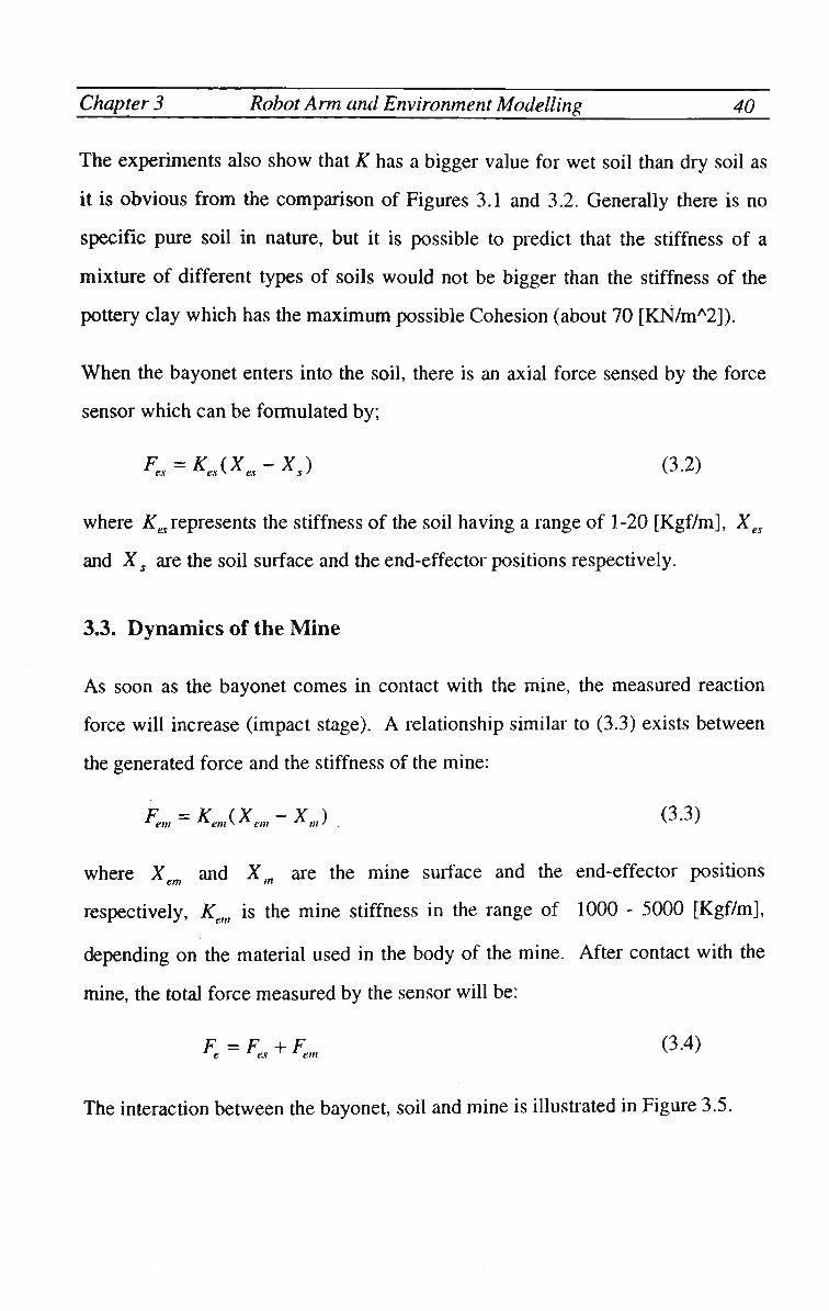
Chapter 3 Robot Arm and Environment Modelling 40
The experiments also show that K has a bigger value for wet soil than dry soil as
it is obvious from the comparison of Figures 3.1 and 3.2. Generally there is no
specific pure soil in nature, but it is possible to predict that the stiffness of a
mixture of different types of soils would not be bigger than the stiffness of the
pottery clay which has the maximum possible Cohesion (about 70 [KN/mA2]).
When the bayonet enters into the soil, there is an axial force sensed by the force
sensor which can be formulated by;
F„ = Ka(Xa-X,) (3.2)
where ^represents the stiffness of the soil having a range of 1-20 [Kgf/m], Xes
and Xs are the soil surface and the end-effector positions respectively.
3.3. Dynamics of the Mine
As soon as the bayonet comes in contact with the mine, the measured reaction
force will increase (impact stage). A relationship similar to (3.3) exists between
the generated force and the stiffness of the mine:
F =K (X -X ) (3.3) em * emv em m' . v '
where X and X,„ are the mine surface and the end-effector positions em tn A
respectively, Kem is the mine stiffness in the range of 1000 - 5000 [Kgf/m],
depending on the material used in the body of the mine. After contact with the
mine, the total force measured by the sensor will be:
F =F +F (3.4) e e.i em
The interaction between the bayonet, soil and mine is illustrated in Figure 3.5.
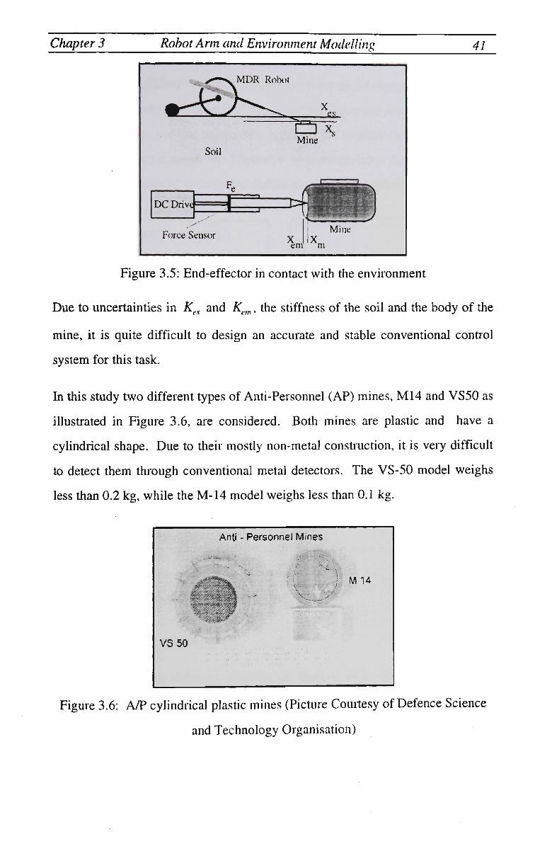
Chapter 3 Robot Arm and Environment Modelling 41
M D R Robot
_____
Q xs Mine
Soil
DC Drive
Force Sensor
em
__/ Mine
m
Figure 3.5: End-effector in contact with the environment
Due to uncertainties in Kes and Kem, the stiffness of the soil and the body of the
mine, it is quite difficult to design an accurate and stable conventional conhol
system for this task.
In this study two different types of Anti-Personnel (AP) mines, M 1 4 and VS50 as
illustrated in Figure 3.6, are considered. Both mines are plastic and have a
cylindrical shape. Due to their mostly non-metal construction, it is very difficult
to detect them through conventional metal detectors. The VS-50 model weighs
less than 0.2 kg, while the M-14 model weighs less than 0.1 kg.
Figure 3.6: A/P cylindrical plastic mines (Picture Courtesy of Defence Science
and Technology Organisation)

Chapter 3 Robot Arm and Environment Modelling 42
The stiffness coefficients of the two mines were measured experimentally and the
results are illustrated in Figure 3.7. The graph (a) shows the relationship between
the reaction force and the penetration depth of the bayonet for the body of the
mine whereas the diagram (b) illustrates such relationship for the fuse of the
mine. The gradients of these curves define the stiffness coefficients.
a)
VS 50 A/P Mine Stiffness
4000
Distance [mm]
b)
./
i % i % i
Figure 3.7: Stiffness coefficients of the A/P cylinder plastic mine body and fuse
(VS 50)
The stiffness coefficient of the body of V S 50 is about 1200 [Kgf/m] which
means the stiffness coefficient of this type of mine is in the order of a few
thousand. The material used for the fuse of the A/P mines is softer than its body.
In addition, the fuse is assembled with a spring which has a lower stiffness
coefficient compared to the material used in the body of the mine. The
experimental results indicate that the stiffness of the fuse is about 10 [Kgf/m].
Therefore, this study will focus on demining various A/P plastic mines with
stiffness coefficients of up to 5000 [Kgf/m].
3.4. Arm/Sensor model
In this section three different methods are applied to model the arm and the
sensor in contact with the environment. Firstly, a mathematical method is
presented which has proved to be unsatisfactory. Then an experimental approach
is reviewed which uses an input/output data set to derive a simplified transfer

Chapter 3 Robot Arm and Environment Modelling 43
function representing the whole system. Finally a neuro-fuzzy modelling
algorithm is described which is employed to derive an intelligent model for the
whole system.
3.4.1. Mathematical Modelling
Developing an accurate mathematical model to represent the mechanical arm and
its interaction with the environment has proved to be a difficult task. In order to
simplify the modelling process, a number of non-linear and complex parameters
of the experimental rig (Figure 3.8), such as friction and backlash, are ignored in
the model. Studying and including every single of these parameters in the
mathematical model in order to design an appropriate controller could be a P h D
thesis. But the aim of this thesis is to focus on intelligent control methods.
Sliding Part
Force Sensor
f Motor 3
fa \Jr,* G(s)
T muffli
Environment
A
x-,
u< > K T
H_>SI_
4
K
KE
1 B+SJT G2
w • » HH
— i
ke
-<
nil bs nh Dynamic M(«lel irfUw Anii/Sensor/Eiiviroiihienf
Figure 3.8: The dynamic model of the manipulator and end-effector
As it can be seen in Figure 3.8, the stiffness and viscous damping coefficients of
the force sensor are considered in the dynamics of the robot. In the following
equations the term *,(*, -x2) describes the stiffness force component detected
by a force sensor and the term k,xy describes the contact force between the end-
effector and the environment.

Chapter 3 Robot Arm and Environment Modelling 44
The term ^(JCJ -X2) also describes the damping component of the force sensor.
mlxl+bs{xl -x2) + ks(xl -x2) = F (3.5)
m2Jc2+^(i:2 -ij) + fcT(jc2 -x{) + kex3 =0 (3.6)
T-Fr, xx - v, , x2 = v2 , v, =o)r (3.7)
where
mi mass of manipulator [kg]
m2 mass of end-effector [kg]
*! position of manipulator (sliding part) [m]
x2 position of end-effector (sensor shaft) [m]
x, deformation of environment in contact with end-effector [m]
manipulator velocity [m/s]
end-effector velocity [mis]
co angular velocity of motor [rad/s]
bs damping coefficient of force sensor [N-s/m]
ks stiffness coefficient of force sensor [N/m]
ke stiffness coefficient of environment [N/m]
F force applied to manipulator [N]
T torque needed to produce force F [NM]
r radius of motor/reduction gear tm]
The torque equation can be written as
Te = JTw + B(o + T (3-8)
l3
Vl
V2

Chapter 3 Robot Arm and Environment Modelling 45
where
B armature viscous damping coefficient [NM-s/rad]
JT load inertia of the servo motor [NM-s ]
Using Equations (3.7) and (3.8) and substituting them in Equations (3.5) and (3.6
) we obtain
v,= K [Te-Bevl + rbsv2-rkx(xl-x2)] (3.9)
v2 = V [b^v.-b^v^+k^Xy-x^-k^] (3.10) / ^v
J B where Je - — + rm{ and Be = — I - rbs
r r
In order to find the transfer function of the total system, first the transfer function
G/s) is obtained. The input and output of G}(s) are the velocity error and the
output torque generated by the motor respectively. For the velocity control loop,
it is assumed that the end-effector is moving in free space and is not in contact
with the environment. Therefore, the terms in Equations (3.9) and (3.10)
resulting from the contact between the bayonet and the environment have no
effect. Using the mechanical model presented in Figure 3.8, the transfer function
of the dc motor (GM (s)) can be represented as;
G(S) = LS?±= KT (3.11)
l W ejs) Ra+SLa
where KT is the torque constant and KE is the back E M F constant of the motor.
The transfer function G2(s) which relates the motor torque to the angular
velocity of the motor can be obtained as follows:
G, (,)_«___) = _ L _ (3.12) 2 T(s) B + SJT

Chapter 3 Robot Arm and Environment Modelling 46
G A / ( , ) = ^M(£1___S U)G2is)
GMis) =
Ur(s) I+KEG^G^S)
AT
LaJS2 + (LaB + RJ)S + iRaB + KTKE)
(3.13)
(3.14)
Figure 3.9 illustrates the block diagram of the dc motor transfer function GM (s),
including the sensor and the arm dynamics. Assuming that the end-effector is
rigid and the arm is moving in free space for a length equal to the difference of
the X3-X2, it is possible to find the resultant force from F = Ke*x2. In this block
diagram KL is the constant to convert the angular velocity of the dc motor to the
linear translation of the sliding part.
u r
— J * OJ.)
D C Motor
WK ?
Velocity of Velocity of End-effector Sliding Part
\
V(K)
}
s.
G(s) s
;nsor & A
V2W
rm
1/s
End-effector Position
X(s) 2 K
Force F >
Figure 3.9: The open loop force model
The transfer function Gs(s) relates the manipulator velocity to the end-effector
velocity.
VJs) bsS + Ke Gsis) = _ r2"
VAs) m2S2+bllS + Kjl + Ke
(3.15)
Finally the open loop transfer function of the whole system including the motor,
manipulator, sensor, and the environment, relating the reference velocity to the
measured force is:
GMFis) = Fs (s) KeKL{\ - G, (.0]G, (s)G2 (s)
Ur(s) S[\ + KEGx(s)G2(s)} (3.16)

Chapter 3 Robot Arm and Environment Modelling
GMF(s) = KeKLKTibsS + Ke) Ft(s) __
Uris) Sia4S4 + A , 5 3 +a2S
2 + «,S + «0)
47
(3.17)
where
fl4 = LaJTm2
a3 = Ltt/rfcv + m2iRaJT + L,,fl),
a2 = LaJTiKs + Ke) + bs(L<lB + RaJT) + in2(RaB + KTKE)
«,=(*,+ Ke)(LaB + RaJT) + bx(RaB + KTKE)
a0 = iKs + Ke)iRaB + KTKE)
In order to study and analyse the effect of the stiff environment on the overall
behaviour of the system, first a classical PID controller is designed for the
velocity control of the dc servo motor as the inner loop of a general explicit force
control structure (Figure 3.10).
19 K -KV*PID
_A
D C Servo Motor
$. k/s Sensor and_J_^ Environmei it
Figure 3.10: A simple explicit force control with an inner velocity control loop
The PID controller is designed to produce minimum steady state error (Velocity
error constant K v = 40), a fast response and an acceptable overshoot (less than
20%) for a unit step response. The step response and the root locus of the inner
velocity control loop of the dc servo system with the designed controller
(kp=10000; kd=326.6; ki=60000) are illustrated in Figure 3.11. It is clear from the

Chapter 3 Robot Arm and Environment Modelling 48
step response, there is less than 2 0 % overshoot (£ « 05) and an acceptable steady-
state error (e„(0.05).
A
m
P I
1
u
a
•
1
OB
0*
I) 2
°
j
j J
J
/ ' '
005 01 U15 0 2 0 25 o:< IK* I 4
9
A
1
2U
U
r '"
•lo*
" -
•41 10
-.
-_
•W -20
^'
-10
ij
1
0 Be (J AWJ,
10 20 SO 40
Figure 3.11: Step response and the root locus of the inner velocity loop using a
PID controller
The root locus of the system illustrates that the closed-loop system of the
compensated system is stable for all the gains. Since the parameters of the
environment have no effect on the motor transfer function, the PID controller is
assumed to have constant parameters for different types of environment.
The force proportional controller K f in Figure 3.10 is designed to be 0.025. As
the output of the force controller provides the set point for the inner-loop, it
should be in the range of the maximum velocity of the motor, which is 0.027
[m/sec]. By including the inner velocity control loop in the total system with the
force proportional control gain of 0.025, the root locus of the system will be as
shown in Figure 3.12. It is assumed that the experimental rig is in contact with an
environment having a stiffness of Ke= 14000 [Kgf/M].

Chapter 3 Robot Arm and Environment Modelling 49
1 m a
g
A X 1
•
400
200
•200
-400
-600 10
\
^ /
40 -10
i ^ - — — -
j - - " " " " ' o 10
Real Axis
"~" 20
-
-
30
Figure 3.12: The root locus of the system with a PID velocity controller
The root locus has complex conjugate poles from which loci moves towards the
right hand of the s-plane. Since the environment in this model is represented by a
constant gain, a stiff environment makes the total system unstable. The system
has complex conjugate poles on the imaginary axis. In order to investigate the
effect of these poles on the system behaviour in more detail, the step response of
the total system with a proportional gain of (Kf=0.025) in the outer force control
loop (Figure 3.13 ) is considered. Figure 3.14 also illustrates the corresponding
velocity for the step response of the total system.
p i i t u 0.8 d
0.2
0.2 0.3 0 4 0.5 0.6 Time (sees)
Figure 3.13: Step response with the proportional force controller (K_=14000,
Kf=0.025)

Chapter 3 Robot Arm and Environment Modelling 50
A m
P 0.02- A
1 t u 0.015;
d e
0.01
0.005
0
-0.005
/ \
-I \ j I j 1
\
" V 0 0.1
^ 0.2
- — — •
0.3 Time (sees)
0.4 O.S
-
0.6
Figure 3.14: Velocity of the motor for the above step response
According to the obtained unit step response, the transient response is fairly fast
with an acceptable overshoot and a settling time of about 0.2 seconds which
represents the response of a stable system. This result is in conflict with the root
locus of the overall system as the closed loop poles for all values of feedback
gains are shown to be in the right half of the S-plane. Hence, the unit step
response should have been oscillatory and unstable.
More investigation is carried out to identify the reasons for such behaviour. The
total transfer function of the system is in the order of six. The total closed-loop
transfer function of the system can be written as:
C(s) K(s + z, )(s + z2)...(s + zj
R(s) (s + PiXs + p^.-is + p,,)
For a unit step input (Ris) = V ) the response of the system will be:
(3.18)
C(s) = a- + i^ (3.19) s j=ls + Pj
in which a} is the residue for the pole at .v = -p}.
As the poles of C(s) can be both real and complex conjugate, it is better to rewrite
3.19 in the following form:

Chapter 3 Robot Arm and Environment Modelling 51
(3.20) S j^xS + Pj k S2 -r-2^(0fc.f+0)A
2
or in the time domain as
q r
c(t) = a + Ysaie~P}t + X V ^ ° * ' cosco* V-Wt 7=1 *=1
r ________
+ X ^ e " ^ 0 * ' sincoA. jl-tft , > 0 (3.21)
Equations (3.20) and (3.21) show that the unit step response of the full system
can be found by the supeiposition of several first and second order step
responses. Using this method, the total closed-loop transfer function of the arm
in contact with the environment is divided into two first order and two second
order transfer functions. The transfer function producing the complex poles on
the imaginary axis at ± 577.4/ is shown below:
__ - 2597 xlO"7(.y + 4.441 xlO'16) + 8.925 x!0~3 3
lm"s-polex ~ s2 + 8.882 x 10"16 s + 3.334 x 10⁵
By comparing Equation (3.22) with Equation (3.20) the parameters of the
components corresponding to poles on imaginary axis will be;
bk = -2597 x 10~7, ck = 1546 x 10
-5,
co, = 577.4, %k = 7.691 x 10"w (3.23)
Since the damping ratio is very small (£,k = 0 ) , the exponential terms in (3.21)
can be assumed as unity. Therefore, the total step response for the transfer
function (3.22) would be a sinusoidal function with the amplitude and frequency
given in (3.23). The step response of this transfer function is illustrated in Figure
3.15.

Chapter 3 Robot Arm and Environment Modelling 52
, X10
A m
P I I I u d e
-6 - J i _ - J 1 — , 1 i i i _
0 0.01 0.02 0.03 0.04 0.05 0.06 0.07 0.08 0.09 0.1 Time (sees)
Figure 3.15: The step response corresponding to pair poles on the imaginary axis
The oscillation of the response due to the imaginary poles seems to be fairly
small compared with the amplitude of the overall response. The amplitude of the
response, however, tends to increase in time, which results in an undesirable
steady state condition. Figure 3.16 illustrates the increasing oscillatory unit step
response of the system after 50 sees.
Figure 3.16: Unit step response of the total system in 50 seconds.

Chapter 3 Robot Ann and Environment Modelling 53
It is clear that the step response in contact with a stiff environment is oscillatory
but with a slowly increasing amplitude. The step response is going to exit from
the limit band of +/-5% after about 40 seconds, which is a long time for a fast
response system. Figure 3.17 shows the step response of the system in contact
with a reasonably soft environment (K_=140) for 10f' and 2*106 seconds. The
step response for 10' seconds (about 12 days) is a satisfactory response but after
that time it starts to increase its oscillatory amplitude, which is not a main issue
for practical applications.
A
»' 1
I 1
u 08 d
or
0*
u;
% 2 t 4 5 f. TrfTi* | » « &)
7 " V 1
«. Hi
0
A
t>
•1
V 2
1
Utf
Oi
Vi
L'l
1 o; 0 4 VH. O B 1 Tirn» (<,*< *
1 2 \ 4 i r.
__,* ^ ^ B ) j
1 6 2
xld
Figure 3.17: The step response for Kd=140 and Kt=0.025
It should be mentioned that in the above results, the stiffness of the environment
is assumed to be constant at 14000 [kgf/m]. In practice, however, such stiffness
can have large variations that will affect the performance of the overall system.
For example, by doubling the stiffness from 14000 to 28000, the step response of
the compensated system has a completely different response (Figure 3.18)
compared to the step response shown in Figure 3.16. It is obvious that the system
would be totally unstable when it comes in contact with this environment. The
reaction force generated is also quite high which can either damage the arm or
trigger the mine.

Chapter 3 Robot Arm and Environment Modelling 54
800 A m p 600 1 1 400 t U d 200 e
0
-200
-400
•600
i 1 i i i
1
i
l
III
111 IM i
0 5 10 15 20 25 30 35 40 45 50 Time (sees) j
Figure 3.18: Step response of the system with the designed PID controller
contacting the stiff environment (ke=28000 [Kgf/m])
By removing the poles on imaginary axis from the total transfer function of the
system, the root-locus of the remaining system is shown in Figure 3.19. This
represents a stable system for all the gain values.
1 m a 9
A X 1 s
6
4
2
t>
-2
-4
-6
xlrf — i —
- /
-
-6
- -i
-4 -2 0 Real Axis
2 1
4
-
6
Xlrf
Figure 3.19: Root-locus of the system after removing poles on imaginary axis

Chapter 3 Robot Arm and Environment Modelling 55
3.4.2. Validation of the Model
The developed model and its controllers are employed to control the experimental
rig. The proportional force controller and PID velocity controller are
implemented using a digital control approach with a sampling interval of T=0.01
[sec]. The following algorithm was used to implement the digital PID
controllers:
/)(_) = A T , + M ( £ ± l ) + £ t ( £ z l ) (3.24) 2 z-1 T z
Where Kp, Ki and Kp are the controller and T is the sampling period of the digital
control loop. Comparing the above PID controller structure with the standard
form of a second order pulse transfer function
results in
a0 = KP+^KIT + KD
a^-Kp+±K{T-^KD
ai=-^KD
bx=-\
b2=0
The result of the experimental work, using the above coefficients, is shown in
Figure 3.20. The output velocity of the inner control loop is quite oscillatory and
saturated between the maximum and minimum velocity of the motor. It is quite
clear that the motion of the bayonet is oscillatory rather than a smooth movement
along a straight line. Moreover, this oscillatory motion has slowed down the
response as it has taken the bayonet 20 seconds to travel a distance of about 10
centimetres, which theoretically should not be less than 2 seconds at the

Chapter 3 Robot Arm and Environment Modelling 56
maximum speed of the motor. Hence, the derived model is not an accurate
representation of the overall system.
Overall, the designed PID controller based on the derived model is completely
oscillatory and out of control even when the arm is moving in free space. This
could be due to ignoring a number of important system parameters, such as
friction, vibration, and backlash, in the model of the system.
Figure 3.20: Behaviour of the system using the designed compensator
Another source of non-linearity and oscillation of the experimental rig could be
the physical limits on the motor velocity which adds a saturation non-linear type
behaviour to the system.
Overall, the derived mathematical model has proved to be unsatisfactory and not
a feasible model to be used in the development of the conhol algorithm. It was
therefore decided to employ a heuristic method known as Adaptive Spline
Modelling of Observation Data ( A S M O D ) [Kav92], to extract a model based on
the input/output data available from the system. The advantage of such a model
is that it can easily accommodate variation in the structure of the system and its
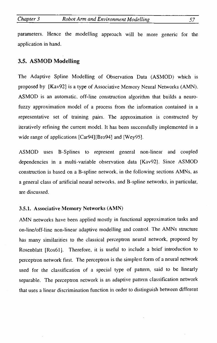
Chapter 3 Robot Arm and Environment Modelling 57
parameters. Hence the modelling approach will be more generic for the
application in hand.
3.5. ASMOD Modelling
The Adaptive Spline Modelling of Observation Data (ASMOD) which is
proposed by [Kav92] is a type of Associative Memory Neural Networks (AMN).
A S M O D is an automatic, off-line construction algorithm that builds a neuro-
fuzzy approximation model of a process from the information contained in a
representative set of training pairs. The approximation is constructed by
iteratively refining the current model. It has been successfully implemented in a
wide range of applications [Car94][Bro94] and [Wey95].
A S M O D uses B-Splines to represent general non-linear and coupled
dependencies in a multi-variable observation data [Kav92]. Since A S M O D
construction is based on a B-spline network, in the following sections A M N s , as
a general class of artificial neural networks, and B-spline networks, in particular,
are discussed.
3.5.1. Associative Memory Networks (AMN)
A M N networks have been applied mostly in functional approximation tasks and
on-line/off-line non-linear adaptive modelling and conhol. The A M N s structure
has many similarities to the classical perceptron neural network, proposed by
Rosenblatt [Ros61]. Therefore, it is useful to include a brief inhoduction to
perceptron network first. The perceptron is the simplest form of a neural network
used for the classification of a special type of pattern, said to be linearly
separable. The perceptron network is an adaptive pattern classification network
that uses a linear discrimination function in order to distinguish between different
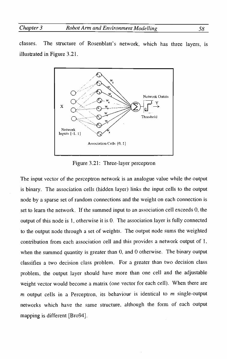
Chapter 3 Robot Arm and Environment Modelling 58
classes. The structure of Rosenblatt's network, which has three layers, is
illustrated in Figure 3.21.
Figure 3.21: Three-layer perceptron
The input vector of the perception network is an analogue value while the output
is binary. The association cells (hidden layer) links the input cells to the output
node by a sparse set of random connections and the weight on each connection is
set to learn the network. If the summed input to an association cell exceeds 0, the
output of this node is 1, otherwise it is 0. The association layer is fully connected
to the output node through a set of weights. The output node sums the weighted
contribution from each association cell and this provides a network output of 1,
when the summed quantity is greater than 0, and 0 otherwise. The binary output
classifies a two decision class problem. For a greater than two decision class
problem, the output layer should have more than one cell and the adjustable
weight vector would become a matrix (one vector for each cell). W h e n there are
m output cells in a Perceptron, its behaviour is identical to m single-output
networks which have the same structure, although the form of each output
mapping is different [Bro94].

Chapter 3 Robot Arm and Environment Modelling 59
The structure of an A M N can be presented by a three layer feed-forward network
including input layer, basis function (hidden layer), and output layer. Figure
3.22 illustrates a B-spline type of a three layer A M N structure.
Coeficient Vector
Figure 3.22: B-spline type of an A M N s structure
The input layer of an A M N is a normalised input space. The shape and size of
the basis functions in the hidden layer represent the main structure and
complexity of A M N s . The output of the basis functions, bt generally is in the
range of 0 to 1. W h e n the output is zero, the associated basis function and the
corresponding coefficient (weight) do not contribute to the output of the network.
In the process of learning the basis functions, their locations (knot) in input space
and corresponding coefficients are adapted to minimise the output error. One of
the differences between A M N s and Perceptron networks is that there is no
thresholding unit in A M N s . The output of the A M N is a linear continuous
combination of the outputs of the basis functions. Therefore, the output of an
A M N , is dependent on the basis functions, /?,U) and their corresponding
coefficients, ct. The output can be represented by:
? = _£>,(*) (3.26)
Chapter 3 Robot Arm and Environment Modelling 60
It is clear from (3.26) that the learning process of an A M N network is a simple
linear optimisation problem. There are several different types of A M N networks
such as, B-spline basis functions, Radial Basis Functions (RBF), Cerebellar
Model Articulation Controller ( C M A C ) and Fuzzy networks. There will be more
detailed discussion on B-spline basis functions will be presented in the
forthcoming sections.
3.5.2. B-spline Basis Functions
B-spline is mostly used in graphical applications as a basic surface fitting element
[Cox90]. As the output of B-spline basis function networks is smooth due to
shape of the B-spline basis functions, there is considerable attraction in using this
class of neural network in nonlinear function approximation, particularly in
modelling and conhol of nonlinear systems. The degree of the B-spline function
determines the shape of the B-spline basis function. A set of B-spline basis
functions is known by a set of knots (vector knots) on the input domain and a set
of coefficients defining the percentage contribution of each basis function to the
output. One dimensional B-spline basis functions of degrees zero (constant), one
(linear) and two (quadratic) are illustrated in Figure 3.23. As can be seen from
the figure, for an input between second and third knots (rj2 and q 3) there are one,
two and three B-spline basis functions contributing to define the output for basis
functions of degrees zero to two accordingly. O n each interval, the basis function
is a polynomial of degree P, and at the knots the polynomials are joined
smoothly. A basis function of degree P, is laid in P+l intervals [Bro94]. It is
important to mention that on each interval, P+l B-spline basis functions and their
corresponding coefficients contribute to the output.

Chapter 3 Robot Arm and Environment Modelling 61
1 _
0.8.
0.6 _
0.4 _
0.2 _
0
Constant B-spline (p = 0)
1
Cl 1 J
0.8 _
0.(i _
0.4 _
0.2 _
1 1 n
1 2 3 4 5
Input Knots
Linear B-spliiie (j> = 1)
c c n L2
AA / V\ /A\ / / \ \
1 2 3 4 Input Knots
Quadratic B-spline (j) = 2)
l j
0.8 _
0.(i _
0.4 _
0.2^
1 0
c c c 1 u2 UJ r\ . \ /->
' Y y \ J \..- i ,-\\ vi \ i
5 1 2 3 4 5 | Input Knots
Figure 3.23: One-dimensional B-spline basis functions (degree 0, 1 and 2) for
the Knot-Vector TJ = (1, 2, 3, 4, 5)
Considering this figure and Equation (3.26), which gives the output of a B-spline
basis function network, it is quite clear that the higher basis functions with
smoother basis function shape lead to a smoother networks output accordingly.
In this diagram, the horizontal axis corresponds to the input space with five knots,
while the vertical axis defines the normalised contribution of each supporting
basis functions for a given input. For example, the output of a linear basis
function for an input located at the second knot (rj = 2) is composed of the
contribution of two linear basis functions and their corresponding coefficients,
which is equivalent to 1 x C, + Ox C2 = C,.
A multi-dimensional B-spline basis functions can be constructed as the tensor
products of one-dimensional basis functions. Therefore, all the properties of the
one-dimensional B-spline basis functions are extended to the multi-dimensional
basis function. The shape of the one-dimensional basis functions determines the
smoothness of the multi-dimensional basis functions and the network output. It is
possible to have different degrees of basis function in each dimension. Figure
3.24 illustrates an example of a two-dimensional B-spline basis function with a
basis function of degree 1 (linear) and 2 (quadratic) in each dimension.

Chapter 3 Robot Arm and Environment Modelling 62
Figure 3.24: A two-dimensional B-spline basis functions with degree 1 and 2 in
each dimension
It is natural to initially define the one-dimensional B-spline basis functions and
then generalise it for higher dimensions.
3.5.3. One Dimensional B-Spline Model
The one-dimensional B-spline basis function of degree P has a support that is
P+l intervals wide. That is, for each input to the network, there are P+l
contributing basis functions used in determining the output of the basis functions.
For example, in Figure 3.23 there are one, two and three basis function supports
for any input between knots 2 and 3 of the basis function from degree zero to
three accordingly. Therefore, the degree of the polynomial approximation
specifies the size of the support of the one-dimensional basis functions. A
general one-dimensional B-spline model is formed as a linear combination of a
set of basis functions, b(x) = (/>_(»,&_(*)> ,bL_{(x))T, and can be expressed by
L-\
I i=0
s(x) = ^cibi(x) = c1b(x) (3.27)
The coefficient vector C=(c 0, c,, ...., cL_x)T represents the set of parameters that
are to be estimated when fitting the model to the data, and the number of
parameters L represents the number of degrees of freedom in the model [Wey95].

Chapter 3 Robot Arm and Environment Modelling 63
The set of basis functions in a B-spline model is uniquely defined by a knot
vector, i - {x0,tp X L + P ) » consisting of an ordered sequence of real values.
Each basis function is a composition of a set of piece wise polynomials of a given
degree p, each defined over disjoint sub-intervals of the input space. The knot
sequence forms a partitioning of the input domain into L+p disjoint and normally
non-uniformly sized intervals, corresponding to the polynomial segments of the
basis functions. The basis function of degree zero (p = 0) can be defined as:
<fr,o(*) = 1> t, < X <T,,, 4,0 ' ,+1 (3.28)
0, otherwise
The following recursive algorithm can be then applied to construct the basis
functions of higher degrees (p = 1, 2, )
h,.M=-^-W>+-^-^ w.<*> <3-29) lj+P Lj li+/'+i L;+i
As is clear from (3.28) and (3.29), the basis function is a piecewise polynomial of
degree P, so the output (3.27) of the B-spline network is also a piecewise
polynomials of degree P.
3.5.4. Multi Dimensional B-spline Models
As mentioned, multi-dimensional B-spline model is formed by tensor product of
one dimensional basis functions, ie:
n-l
n 1=0
«**)=rp*<*/> (330)
where b{ (x{) are the one-dimensional basis functions.
For example, two one-dimensional models with functions bm(x0),
m = (0,l,....L0-l) and />„(*,), n = (0X....Ll -1) respectively will form a two-
dimensional tensor product model with the basis functions defined as:

Chapter 3 Robot Arm and Environment Modelling 64
bm,fM0fxl) = bmix0)bll{xl)
The L()Li two-dimensional basis functions are completely defined by the knot
vectors for the two input dimensions.
The number of basis functions of degree P, defined on an axis with L, internal
knots is (L- + Pt +1). So the total memory requirements for a multi-dimensional
B-spline network is given by:
/V = n(I, + /?+l) (3.31) 1=1
where n defines the size of the input space.
It is clear from (3.31), the size of a multi-dimensional B-spline network is
exponentially dependent on the size of the input space, which would indicate that
multi-dimensional B-spline networks are suitable for low dimensional modelling
tasks. But this problem is overcome by A S M O D algorithm which models a high
dimensional input space as a sum of several low dimensional sub-models.
3.5.5. The ASMOD Model Presentation
In the A S M O D algorithm the output of a model with multi-input variable is
modelled as a sum of several low dimensional sub-models, where each sub-model
depends only on a small subset of the input variables. The decomposition of the
high dimensional input space into low dimensional additive sub-spaces makes the
model transparent to the user, and at the same time the complexity (number of
parameters/coefficients) of the model is dramatically reduced. Another attraction
of the A S M O D algorithm is that the derived model could be represented as a set
of fuzzy rules (linguistic rules) which define the relationship between input
variables and their dependencies or independencies. This makes the model more
transparent to the user [Bos95].

Chapter 3 Robot Arm and Environment Modelling 65
The number of basis functions and hence the number of parameters in the model,
grow exponentially with the dimensions of the input space. If there is an internal
correlation between the input variables one or more of the variables can be
eliminated from the input vector, which will reduce the size of the model. These
possibilities for model size reduction are utilised in the A S M O D modelling
scheme by modelling the data as a sum of several low dimensional models using
only the input variables, which are shown to contribute towards the target values.
Smaller the size of a model, less memory and processing time are required, which
leads to faster on-line learning.
An ASMOD model is constructed as a sum of U one-dimensional and/or multi
dimensional B-spline models, {suixu)}, expressed by
m(*) = |>_U_) (3.32) M=0
Xu represents low dimensional input vectors with disjunct subsets of variables in
the model input vector x. One input variable can hence appear in only one of the
sub-model input vectors, and some of the variables may not be included at all. In
order to make it clearer, an A S M O D model of a system with five input variables
is shown in Table 1.
Table 1: An example of A S M O D model.
Sub-model 1
Sub-model 2
Sub-model 3
Sub-model 4
Input Variables
3 1
2
5 4
Spline-degree
2 2
2
1 1
In this model there are three one-dimensional sub-models for the input variables
3, 5, and 4, and one two-dimensional sub-model for the input variables 1 and 2.
As can be seen, the degrees for B-spline basis functions are different. Figure

Chapter 3 Robot Arm and Environment Modelling 66
3.25 shows the basic structure of the A S M O D model of the example presented in
Table 1.
x,—
x.—
** —
x,—
x,—
/xxxxxxxxx
/X>OOOOOOC\
yxxxxxxxxx y>c*XYXyxyx^
VXvXvXyXvXy
s _ \
jC_v—>
7
Figure 3.25: The A S M O D algorithm structure for the example presented in
Table 1
In order to see how ASMOD can be mapped into a neural network architecture,
(3.32) can be expanded with an expression for each sub-model of (3.27);
w-l M-1 L-\
«(*) = _>_ X„ (*_) = _£_>_ Cihi (•*«) (3.33)
«=o M=() 1=0
which results in:
mix) = y£crb,.(x) (3.34)
The sum is taken over all the basis functions and the corresponding coefficients
in the model. Equation (3.34) compared to Equation (3.26) corresponds exactly to
the transfer function of a three layered feed-forward neural network, with one
linear output node and a separate node in the non-linear hidden layer for each of
the B-spline basis functions in the model. The coefficients (weights), location
and the shape of the transfer functions of the hidden layer are implicitly
determined by the model structure as given by the knot vectors.

Chapter 3 Robot Arm and Environment Modelling 67
3.5.6. A S M O D as a Neuro-Fuzzy Algorithm
In the literature, the B-spline basis function networks in general and A S M O D in
particular, are categorised as neuro-fuzzy networks/algorithms. In this section, it
will be made clear why A S M O D is a neuro-fuzzy type network. It is also
important to know the benefits of combined neural networks and fuzzy networks.
The complimentary characteristics of neural networks and fuzzy systems [Bos95]
have authorised the positive attributes of both approaches to be combined. The
combined system is known as a neuro-fuzzy system since it embodies the well
established modelling and learning capabilities of neural network with the
transparent knowledge representation of a fuzzy system.
In particular, it has been shown that B-spline networks and certain forms of fuzzy
systems are equivalent [Bro94]. In order to see the similarity between a fuzzy
and the B-spline networks, the fuzzy set and fuzzy algorithms are defined first.
A fuzzy set A is defined on a universe of discourse X (Figure 3.26), and the
membership function \iA:X —> [0,1] assigns to each element xe X a real number
p.A(;c)in the interval [0, 1] which is:
A = {(x,\LAx))\xeX) (3.35)
•H-W
-4 -3 - 2 - 1 0 1 2 Universe of Discourse
3 4 x
V
Figure 3.26: A typical triangular fuzzy membership function

Chapter 3 Robot Arm and Environment Modelling 68
A fuzzy algorithm is normally presented by a set of rules using fuzzy (vague)
terms (A*) such as small, medium or large to map the input variables to the
output variables. A fuzzy algorithm is composed of fuzzy rules of the form:
IF ixx is A[) AND AND (JC„ is A,;) THEN (y is Bj) (C(/) € [0,1]
where confidence or coefficient Cy determines the contribution of each rule
(membership function) to the output. A fuzzy rule maps the antecedent, formed
by the intersection (AND) of n linguistic statements ixk is A\), to the consequent
formed by a single linguistic statement (v is B J ) . Therefore a set of fuzzy rules
presenting a system could be in the form of:
r..: IFiXisA^THENiyisB') (c^e.O, 1]
where ri} represents the ij'h fuzzy rule and A' is the i'h multi-dimensional fuzzy set
formed from the fuzzy intersection of the individual one-dimensional fuzzy set.
If the fuzzy algorithm has n input and m output variables, it can be presented as m
fuzzy algorithms each with n inputs and one output [Bro94].
B-spline basis functions can be used as the fuzzy membership functions by
defining the degree of the basis functions and the knot vectors. The knot vectors
determine the size of the knots interval and hence define the width of each fuzzy
set on the original input space. For example, if a basis function of degree one
iP-1), is used to define the rih one-dimensional fuzzy set membership function
u^ (•), a knot vector including P+2 knots (rj;I_2 !)„_, T)„) should be defined and the
n'h membership function could be found using (3.28) and (3.29).
Hi (•) = *„,(*)
As is shown in Figure 3.23, this basis function has the popular triangular shape
used in many fuzzy logic implementations. It is clear how B-spline basis

Chapter 3 Robot Arm and Environment Modelling 69
functions can be used to represent the fuzzy membership functions which
implement the fuzzy linguistic terms.
Fuzzy rules can be extracted from B-spline basis function networks (ASMOD
model), first, by assigning a fuzzy linguistic label to each of the input one-
dimensional basis functions. The product operator which combines the one-
dimensional basis functions represents a fuzzy conjunction ( A N D ) and addition is
used as the fuzzy disjunction (OR) operator. Therefore, by ORing the sub
models basis functions and ANDing of the one-dimensional input sets in a multi
dimensional sub-model, the antecedent of the fuzzy rules can be produced. Then,
an evenly distributed fuzzy membership function, including five or seven basis
functions, can be used as the output fuzzy sets (Figure 3.27). Finally, all the
possible input variables should be fired to find the A S M O D model output in
order to associate them to the linguistic fuzzy output sets. It is quite clear that a
coefficient would be obtained for each rule in order to establish a correct
mapping from the input space to the output space. More detailed explanation of
extracting rules from the A S M O D model can be found in [Bos95].
^(y)
l
0.92 '
0.21 0
Neg. Neg. Pos. Pos. Large Small Zero Small Large
y
Figure 3.27: Linguistic fuzzy output sets
For example, the multi-dimensional B-spline network illustrated in Figure 3.25
can be interpreted as a set of fuzzy rules as below;

Chapter 3 Robot Arm and Environment Modelling 70
r]2: IF (x3 is very large)
A N D IF (x, is very small) O R (x2 is very large)
A N D IF (x5 is small)
A N D IF ix4 is medium) T H E N (y is Pos. large) (c]2)
where ry refers to the y* fuzzy rule and c.. is the coefficient associated with each
rule. It should be mentioned that the presented rules are just an example for each
sub-model in Figure 3.25. Depending on the number of basis functions and
knots vector, it is possible to derive more rules.
The interpreted fuzzy linguistic rules for this model make the unknown system
more transparent, particularly when the knowledge about the control of the
system cannot be easily obtained from the human operator. By constructing an
A S M O D model from the data obtained from a system controlled by an expert
operator, it is possible to convert the A S M O D model to its equivalent linguistic
fuzzy rule. This similarity between A S M O D models and Fuzzy models could be
also useful in integrating fuzzy linguistic rules into A S M O D model. The fuzzy
linguistic rules defined by a human operator for a system can be added as prior
knowledge to the A S M O D model.
3.5.7. ASMOD (Neuro-Fuzzy) Model Construction
The method of constructing an A S M O D model from the training data is
described in detail in this section. The training data is produced while the arm is
energised by a square wave command to insert the end-effector into the soil using
the experimental rig set up. The first step to model the total system is to acquire
input/output data and use it to construct an A S M O D model. The data was
obtained by inserting the end-effector into different types of soil and environment
including the body and fuse of a mine. The contact force, travel distance, and the
arm velocity were recorded as the output of the system during the experiments.

Chapter 3 Robot Arm and Environment Modelling 71
As the second step in the modelling task, data were combined randomly and then
divided into two sets as "train" and "test" data. A n A S M O D model can be
constructed either according to the desired initialisation set up including the
number of sub-models, internal knots, and the type of B-splines or leaving all
initial conditions as empty data. Then, the A S M O D algorithm builds a B-spline
representation for the model, which automatically is adapted to the structure and
dependencies in the data. In this thesis, several different topologies were
examined in order to find the best A S M O D model with the best performance of
the model. The A S M O D algorithm evaluates the performance of the constructed
model based on the normalised root mean square error between the model output
and system output. Details of this work will be discussed in Chapter 4.
As an example, the structure of an A S M O D model constructed for a neuro-fuzzy
adaptive gain controller is illustrated in Figure 3.28.
1 G r 0.9
a 0£ d e 0.7
0.6
0.5
0.4
0.3
02
0.1
0 — -0.4
V \ / \ /
\ / \ /
v x A / \ / \
/ \ -0.2
Submodel no. 1
\ A \ A i
\ A / \ / \ /
V V A A A A / \ / \
/ \ / \
/ V 0 02 dx [mm]
A \ \ / \ /
V A A / \
/ \
)l. 0.4
/ /
\ . 0.6
1 G r 0.9
> e 0.7
0.6
0.5
0.4
0.3
0.2
0.1
r \ \
'
' /
V
/' \
[
Submodel no. 2
A A /\ \ \ \
\ \ \ WW \ V V V
A A h A /x I /\ /
/ \ /
VV V -500 0 500 1000 1500
<«m
i / /
/ /
\
\
\
,\ 2000 2500
Figure 3.28: A n Example of a Neuro-Fuzzy Model
From this Figure, it can be seen that this model has two sub-models for the
variation of the distance and force as inputs. There are also three internal knots
for the linear B-splines (P = 1) in each sub-model.

Chapter 3 Robot Arm and Environment Modelling 72
3.5.8. A S M O D (Neuro-Fuzzy) Model Validation
Validation is one of the important steps in learning design procedures in neural
modelling. It is important to have a performance index to evaluate the neural
network performance with real-world data. One of the simplest but not reliable
methods [Bro94] is reproducing the training data using the constructed model. It
is, however, more realistic and accurate to split the input/output data into training
and testing sets, to evaluate the constructed model by the test data. This method
is used here to validate A S M O D model as part of the overall control system. The
constructed model which is actually an inverse model of the environment is
validated in an adaptive gain control loop method. The output of the A S M O D
model is used to adapt the gain of the proportional force controller illustrated in
Figure 3.29.
^
)-> K ^
ivj
/
i
ASMOD Model
PI Controllei
-•
4 1
Robot Ann
[Speed
Dis. K e
Force
Figure 3.29: Neuro-fuzzy adaptive gain control system
A proportional force controller with the gain coefficient Kf is designed to drive
the arm in free space. The total gain of the outer (force) loop is obtained by
multiplying a constant proportional gain with the adaptive gain KA produced by
the A S M O D model:
KT = Kf*KA (3.36)

Chapter 3 Robot Arm and Environment Modelling 73
It should be mentioned that the transfer function of the motor is obtained,
experimentally, using the general form of the position transfer function of a dc
servo motor [Oga97] given as:
GiS) = K pos Xis)
Eannis) SiTS + l) (3.37)
In this transfer function Kpos and Tm are the gain and time constant of the dc
servo motor. Figure 3.30 illustrates a few seconds of the open-loop position step
response of the system which is used to find the time constant of the system.
60 D 1 s 50
P
' 40 a c e 30 m e n 20 t
[mm] 1 ' 10
0 (
Step response of the system
\ \ \ \ \-—jf
yr : : : :
•
•• j -
) 02 0.4 0.6 0.8 1 1.2 1.4 1
T = 0.07 sec T i m e [secl
6
Figure 3.30: Open-loop position step response of the drive system
The gain of the system is also obtained from the closed-loop velocity step
response of the system (Equation 3.38). The final (steady state) speed of the
system corresponds to the gain of the system.
VU) = Kwl (338) £„„„(•*) T„,S+l
Based on the experimental results, the velocity transfer function of the
manipulator can be represented by 3.39:
0.003 G„,JS) =
5(0.075 +1) (3.39)

Chapter 3 Robot Arm and Environment Modelling 74
This transfer function is used in order to design a PI controller as the inner
velocity control loop, as shown in Figure 3.29.
The performance of the controller is validated through computer simulation. In
order to simulate the proposed control system using SIMULINK, it is assumed
that an A P mine is located one centimetre under the ground with a stiffness of 10
[Kgf/m]. The stiffness of an object expected to collide with the arm is assumed
to be 5000 [Kgf/m] for simulation result given in Figure 3.31. The desired force
is assumed to be 1 [kgf]. The environment is modelled as a switch in which gain
changes between two constant values. The force and velocity of the arm end-
effector which are under control are presented as the simulation results.
._ 1(r SnaiMNm Rmut <i NFAG wtwvi SHIt*** SwiMms itt«i 10 to 5000 SirmtaUii Rwsi* ti NFAG «*i«l SlWriros Swikrlws Inwn 10 hi 2500
[Kff»]
i r - — - - i — 1 1 1 i i i i 1.5
Figure 3.31: Simulation Results when stiffness is switching from 10 to 5000
As is clear, when the arm end-effector comes in contact with the stiff object, the
resulting force increases suddenly, which is controlled by applying the adaptive
gain introduced by the proposed controller. In the worst case, when the arm end-
effector is reaching from soil to the mine with a stiff object (Ke = 5000), there is
an approximately 2 0 % overshoot.
According to the simulation results, the constructed A S M O D model which
defines the adaptive gain is capable of overcoming the problem of non-linearity
of the system when it collides with a stiff environment. Whereas, using the

Chapter 3 Robot Arm and Environment Modelling 75
proportional gain controller designed to drive the motor in free space, the
behaviour of the control system is completely oscillatory and out of control when
the arm collides with a stiff environment.
3.6. Conclusion
In this chapter, the robotic arm and its environment were modelled using
mathematical and heuristic methods. The mathematical model proved to be an
insufficient model to represent the dynamics of the system. This was caused by
the fact that some complex and non-linear properties of the system, such as,
backlash, friction, vibration and saturation were not included in the model. The
validation results proved that the PID controller response was oscillatory while its
simulation response was, at least, a satisfactory response.
The heuristic model was based on a neuro-fuzzy algorithm known as Adaptive
Spline Modelling of Observation Data ( A S M O D ) . This model produced more
satisfactory results. It was also shown that an A S M O D model was very similar to
a conventional fuzzy model providing a better understanding of an unknown
system. The neuro-fuzzy models could be used in a model based control strategy,
which will be discussed in more detail in Chapters 4 and 5.

Chapter 4
DESIGN OF PROPOSED INTELLIGENT IMPACT
CONTROL METHODS

Chapter 4 Design of Proposed Intelligent Impact Control Methods 77
4.1. Introduction
Recent progress in intelligent control using neural network, genetic algorithms
and fuzzy logic control has provided feasible solutions for modelling, and control
of complex nonlinear systems. Such systems have traditionally been studied
using adaptive and optimal control techniques mainly after they have become
linearised. Linearising a system, however, does not always reflect the true
dynamics and physical properties of a system [Har94].
As part of this new trend in intelligent control, a powerful paradigm known as
"neuro-fuzzy" has been developed which is a combination of neural network and
fuzzy logic. The main strength of the Neuro-fuzzy control method is the fact that
it benefits from the properties of both of the paradigms that it has emerged from
(eg., learning and fuzzy linguistic rules). The method has been extensively used
in many applications [Bro94], [Oma96] and [Sha97a] to model, identify, and
control nonlinear complex systems.
As discussed in Chapter 3, A S M O D algorithm which is employed in this thesis,
is primarily a neural network modeling and control method. Due to the similarity
of the B-spline basis functions used in the A S M O D algorithm and the fuzzy
membership functions, and also the possibility of integrating fuzzy rules into the
A S M O D algorithm, this method is generally referred to as a neuro-fuzzy
modelling and control method.
In this chapter, initially the concept of impact control is introduced. Then a
simplified model of the impact and its sources are discussed. Based on the
described control schemes and the results obtained from impact analysis, some
guidelines are derived for the design of the control methods used in this work.
Subsequently, the basics of the neuro-fuzzy control and different intelligent

Chapter 4 Design qf Proposed Intelligent Impact Control Methods 78_
control structures are presented. Then, the procedure employed in the design of
the three proposed impact control schemes is presented. Finally the performance
of the developed algorithms will be studied and compared against each other.
4.2. Impact Control
As it is discussed in previous chapter, impact phenomena is an important issue in
the field of robotics particularly when the robot is approaching a stiff
environment. The transitions between the conditions of free motion and
constrained motion which induces an undesirable reaction force, is called impact
phenomenon. In order to design an impact controller the impact dynamics should
be studied. The impact dynamics model is presented in next section which helps
to draw some guidelines for impact control particularly for the A P mine detection
task.
4.2.1. Impact Dynamics Model
When an end-effector comes into contact with the environment, the induced
impact force acts for a short period of time. The classical methods of impact
analysis are based on the laws of the conservation of momentum and energy
[Gol60]. These laws can be used to study the changes in velocity of each body
involved in the collision before and after the impact, and exchange of energy
during the impact. The impact collision is equivalent to one half oscillation of a
lumped parameter spring-mass-damper system, which is shown in Figure 4.1.

Chapter 4 Design of Proposed Intelligent Impact Control Methods 79
Figure 4.1: Impact Dynamic Model
The two bodies with masses of M} and M2, move respectively at velocities V} and
V_. The measure of the energy loss, as given by the coefficient of restitution (e),
could be assumed to be equal to one, according to the law of conservation of
energy [Tor96]. The impact momentum is:
jF-dt = M^n -Vn)-M2(V2l-V22)
Mi Mi (4.1)
where
F is the impact force,
e is the restitution coefficient which is assumed to be one,
Vn, and V]2 denote the velocity of mass (M_) before and after impact
respectively,
and i is the duration of impact.
Since the duration of impact is short, the impact could be assumed as a pulse of
magnitude J and duration h as given by [Tou89]:

Chapter 4 Design of Proposed Intelligent Impact Control Methods 80
Jh = )Fdt = ie + l) M^ (Vn-V21) (4.2) o (Ml + M2)
where h should be chosen less than x (eg h=0.5x).
In a particular mechanical system approaching an environment, the. masses Mj
and M_ are constant. Hence according to Equation (4.2), the magnitude of the
pulse generated by the impact force is proportional to the velocity of the masses.
In this study, the mechanical arm is the only moving mass as the environment is
stationary. Therefore, the single dominant factor in this relationship is the
velocity of the moving arm. This implies that a faster moving arm results in
shorter duration impacts, which in turn makes the task of the control algorithm
more difficult. The duration of an impact also dictates the maximum sampling
time in the computer control system. It is obvious that the mass of a mechanical
arm should be minimised to obtain less impact force for the same arm velocity.
Considering the original required specifications of the mechanical mine detection
arm, it is more desirable to have a faster insertion of the bayonet into the soil.
This may induce larger impact forces with shorter duration. Therefore, it is
crucial to have an impact control scheme without delay, capable of coping with
the unexpected stiffness variation while minimising the induced impact force. On
the other hand, it is necessary to maintain the velocity as high as possible to
reduce the time required to detect an A P mine.
4.2.2. Impact Control Guidelines
Considering the reviewed impact control methods, the dynamic model of impact
and the characteristics of a robotics deminer, the following guidelines for a
proper impact control method are suggested in this work:

Chapter 4 Design of Proposed Intelligent Impact Control Methods 81
• It is desirable to move the arm as fast as possible in order to speed up the mine
detection process.
• It is desirable not to have more than 2 0 % or, in the worst case, 4 0 % overshoot
as it may set off the mine.
• It is not possible to slow down the arm before contact phase using a vision
system [Nel95] or a proximity sensor in conjunction with the force sensor
[AU92]. Therefore, the speed of the free motion and constrained motion will
be the same, unless the impact control mechanism can reduce the velocity to
minimise the induced impact force.
• The control algorithm should cope with the unknown parameters of the
environment.
• The mass of the aim end-effector should be minimised to reduce the impact
force.
4.3. Neuro-Fuzzy Control
In recent years, intelligent control in general and neuro-fuzzy control in
particular, have been quite inspiring paradigms for real time control applications
[Oma96]. Intelligent control methods normally have properties such as learning
ability, flexibility, robustness, and nonlinearity, which make them quite attractive
in complex systems.
Neuro-control is a scheme based on artificial neural networks which imitate the
biological brain information processing mechanism. Neural networks with the
ability to learn from input-output non-linear functions are employed as good
candidates to solve complex non-linear control problems [Asa90], [Moo93],
[Was93] and [Kav92]. Neurones are basically non-linear elements and hence,
neural networks are basically non-linear systems which can be used to learn and
solve non-linear control problems, usually too difficult for traditional and

Chapter 4 Design of Proposed Intelligent Impact Control Methods 82
conventional conhol methods to handle. The neuro-controllers can realise non
linear control algorithms, and are robust to noise, complexities, and variations in
the plant. According to Omato et al [Oma96], the neural networks are ideal in
process control as they have the following properties:
• Ability to learn any function provided there is enough training data.
• Ability to m a p non-linearly.
• Ability to control under a wide range of uncertainties.
• Possibility of implementing Neural Networks on a Parallel computing
platform.
Neuro-fuzzy control has also been applied to force/impact control, which is a
non-linear complex controller [Ara96], [Bog93], [Kig95], [Kim95], [Mas96],
[Shi96], [Suh94b], [Suk96], [Tar97] and [Yon93].
A neuro-control structure usually has a learning and adaptive mechanism to adapt
to variations in the process parameters. Depending on the applied structure for
learning and control mechanism, there are two major types of intelligent
(adaptive) control structures; direct and indirect adaptive control. There have
been references to other types of structures in the literature [Oma96], but they
eventually fit into one of the two major approaches.
4.3.1. Direct Neuro-fuzzy Adaptive Control
The learning mechanism in this neuro-fuzzy controller adapts itself according to
the performance of the plant. The learning mechanism behaves as a critic,
evaluating the current state of the plant and adapting the control signal through
the performance index and the model [Bro94]. By measuring the output of the
plant and comparing it with the desired set point, error and change (derivative) in
eiror may be calculated. The performance index is estimated based on the error

Chapter 4 Design of Proposed Intelligent Impact Control Methods 83_
and change in error, and is used to adapt the model and controller accordingly. A
general structure of the direct neuro-fuzzy adaptive controller is illustrated in
Figure4.2.
Desired Output +/-
/
V.
"V
— *
Performance Index
]
? e
.-earning mechanism y
Neuro-£ugzy Cpfffrollei
& u
~\
Plant Model
// J
Output Plant
Feedback Loop
y
Figure 4.2: A general structure of a direct neuro-fuzzy adaptive controller
In this approach, the parameters of the controller are directly adjusted to reduce
the output eiTor between the plant and the reference model. The parameters of the
plant are estimated according to the analysis of error. The controller is then
chosen based on the assumption that the estimated parameters represent the true
values of the plant parameters. In brief, in this type of controller, the neuro-fuzzy
system is used directly as the controller.
4.3.2. Indirect Neuro-fuzzy Control
In an indirect adaptive fuzzy controller, a neuro-fuzzy system is used as the
model of the plant to design the controller [Wan93]. The parameters of the plant
are estimated and the controller is chosen assuming that the estimated parameters
represent the true values of the plant parameters. In this type of neuro-fuzzy
controller, a separate adaptive neuro-fuzzy model is constructed to model the
dynamics of the plant. A design procedure is then used to calculate the control
signal.

Chapter 4 Design qf Proposed Intelligent Impact Control Methods 84
The architecture of an indirect neuro-fuzzy adaptive controller is illustrated in
Figure 4.3. There are two feedback loops in this structure; the negative feedback
controller loop and the model/controller adaptive loop. The model/controller
adaptive loop uses input/output observation data to adapt the process model and
adapt the controller accordingly. While, the controller loop uses just the output
observation to compare with the desired output and send the difference (error
signal) to the controller. In this architecture, a neuro-fuzzy model is used to
model the unknown dynamics of the plant, and predict the current state of the
plant from the previous values of state and conhol signal.
Predicted Current State (PCrS)
Controller Design
__k_ Desired Current State (PCrS) Menro-Fuzzy
Controller
Fuzzy/Neural Model
Previous State (PS)
(CnS),
Control Signal
Plant Output
Feedback Loop
Figure 4.3: Structure of an indirect fuzzy adaptive control system.
The information that should be provided for the controller could be a desired next
state, in which a reference model or desired trajectory must also be included in
the architecture, or it could be a step input and the structure of the controller must
contain information about the desired response of the system [Bro94]. The time
constant of the model/control adaptive loop should be longer than the time
constant of the conhol loop, which is determined by the sampling time of the
output data. The model should be adapted at a reasonable rate in order not to
miss any changes in the system dynamics. O n the other hand, it should not be
adapted at a rate to include measurement noise in the model. Therefore, it is

Chapter 4 Design qf Proposed Intelligent Impact Control Methods 85
necessary to have a slower adapting rate compared to the sampling rate used for
the controller. It is worthwhile to mention that, confusingly, some researchers
[Oma96] and [Hun92] refer to this method as direct inverse control.
4.4. Design of Adaptive Indirect Neuro-Fuzzy Controller
In a neuro-fuzzy conhol system the model of the plant is constructed. This model
should relate the deterministic input signals (previous state values and control
signals) to the deterministic output (current state value). Figure 4.4 illustrates an
on line feedforward learning network.
u(t)
Control Signal
?
Feedforward
Plant Model
Previous State
Plant
y(t)
Predicted Current State
y(t)
Figure 4.4: A n online Feedforward Neural Network Model
A neuro-fuzzy model forms a nonlinear mapping if the input signals are
representative and rich enough (meaning that data includes all dynamics of the
system), otherwise it is not able to store the data and learn the unknown
functions. In a given neuro-fuzzy model which has learnt to associate the past
states and control signals with the current state, the control design procedure aims
to produce a controller that can calculate the control signal necessary for the plant
to achieve the desired dynamic response. According to the structure shown in
Figure 4.3, the controller implements the following relationship;

Chapter 4 Design of Proposed Intelligent Impact Control Methods 86
DCrS iPSx DCrS)-^ CnS (4.3) PS Controller CnS
Model PCrS
where PS, DCrS and CnS represent Previous State, Desired Current State and
Control Signal respectively.
The neuro-fuzzy plant model maps the following relationship;
i PS x CnS) -> PCrS (4.4) ~
where PCrS represents Predicted Current State.
Comparison of (4.3) and (4.4), indicates that the controller function is an inverse
model of the plant model [Bro94]. This implies that the trained inverse neuro-
fuzzy model could be configured directly to control the plant. Therefore, the total
transfer function across the controller-plant would be a unity transfer function,
which maps the desired output to the real output. Using the inverse model as the
main block in the neuro-control approach is one of the most widely applied
schemes. Miller et al. provides a number of examples of this method mainly in
robotics applications in his book, Neural Network for Control [Mil90]. This
approach has a long history in the traditional self-tuning control schemes [Ast95],
where the control output to the plant can be obtained from the inverse
mathematical model of the plant by giving the desired plant output. According to
Omatu [Oma96], another reason for the popularity of this approach is its
simplicity.
It is important to mention that this method is highly dependent on an accurate
inverse model of the plant. The role of the neuro-fuzzy modelling system is to
update the plant model on any possible discrepancy between the desired output
and the actual output (online learning). Meanwhile, the control feedback signal
tries to compensate for the model error.

Chapter 4 Design of Proposed Intelligent Impact Control Methods 87
The assumption is that the neuro-fuzzy model approximates the input-output
mapping of the system being modelled precisely. In the real world, however,
factors such as modelling error, dynamical changes or measurement noise, will
induce a discrepancy eyit) between the estimated output, yit) and the system
output yit).
eyit) = yit)-yit) (4.5)
Mean Square Enor (MSE) performance function, given below, is the most
common criterion used to improve the performance of a neuro-fuzzy model.
J = Eie2yit) = ~fje2yit) = ^iyit)-y(t))
2 (4-6)
where E is the Expectation function. This criterion puts a higher emphasis on the
modelling error in the region of the input domain with high probability of
observation compared to the region of low probability [Kav92].
The learning mechanism in a neuro-fuzzy modelling technique is used to
minimise the error eyit) in Equation (4.5). Considering Equation (3.23), which
defines the output of an B-spline network model, the coefficient vector crcan be
adjusted to minimise the enor. The output of the neuro-fuzzy model is linear
with respect to the coefficients as shown in Chapter 3. Hence linear optimisation
techniques, such as Error Correction (EC), Gradient Descent (GD), and
Stochastic Approximation, can be used to optimise the coefficients of the B-
spline basis functions to improve the performance of the model. Kavli [Kav92]
has used the stochastic approximation version of the L M S (Least Mean Square)
rule as a learning technique for the A S M O D algorithm. The stochastic
approximation scheme is a general iterative algorithm for finding the parameter
vector, cr, minimising enor in the function given by (4.6). It is important to note

Chapter 4 Design of Proposed Intelligent Impact Control Methods 88
that in stochastic approximation, which is capable of filtering out the
measurement and modelling noise, the learning rate is slowly reduced through
time, which results in a faster convergence rate [Bro94].
4.4.1. Neuro-fuzzy Controller Design Based on the ASMOD Algorithm
The A S M O D algorithm has been applied to a wide variety of modelling
problems; robot actuator modelling, metallurgic process modelling, water content
estimation and redundant functional approximation [Kav92]. It has been bench-
marked against multi-layer perceptron, radial basis function and partial least
square networks, and appeals to perform at least as well as the best of the other
models [Bro94].
To design a neuro-fuzzy intelligent conhol based on A S M O D algorithm, an
inverse neuro-fuzzy model of the plant should be constructed first. Then, based
on the constructed model, several conhol structures can be presented. In the next
section the A S M O D model construction is discussed.
4.4.2. Inverse ASMOD Model Construction
In order to construct an A S M O D neuro-fuzzy model of the robot arm used in the
mine detection task, it is necessary to generate sufficient input/output data pairs
to train the model off-line as shown in Figure 4.5.
Q
InVei Neurdfuzzy Motel
Training Mechanism
Robot Ann
Figure 4.5: Off-line inverse training mechanism

Chapter 4 Design of Proposed Intelligent Impact Control Methods 89
As mentioned before, the aim of the training mechanism is to minimise the M S E
error between the output of the constructed inverse model and the required signal
to drive the robot. A set of experiments should be performed to measure the
position/velocity and force of the arm with the associated applied signal to the
robot arm, as the input/output pairs. In order to have a complete set of data
covering the universe discourse, it is necessary to organise as many different
situations as possible to experience various induced forces from environments
with different characteristics. This is vital to the model generalisation. As there
are two different types of models used in the proposed control schemes, the
procedure used in the construction of each model will be described in the
following sections.
4.5. Intelligent Impact Control Design
In this section three intelligent impact conhol methods are studied. There could
be different control configurations depending on the model construction and the
structure of the controller applied to the robot arm. Generally, the conhol
structure for all the proposed methods is inspired from the explicit force control
method in which an internal velocity or position control loop is placed inside the
outer force loop control. The first method presented here is based on a simple
gain scheduling technique. W h e n the arm comes in contact with different types of
environments, it experiences different gains which leads the controller to adapt
the gain of the force control loop accordingly. This method is called Neuro-
Fuzzy Adaptive Gain controller ( N F A G ) and estimates the changes in
environment stiffness. In the second method, a neuro-fuzzy inverse dynamic
model of the robot arm in contact with the environment is applied to control the
impact force of the arm searching for A P mines. This method is called Neuro-
Fuzzy Impact Control (NFIC). Finally, another intelligent control method,
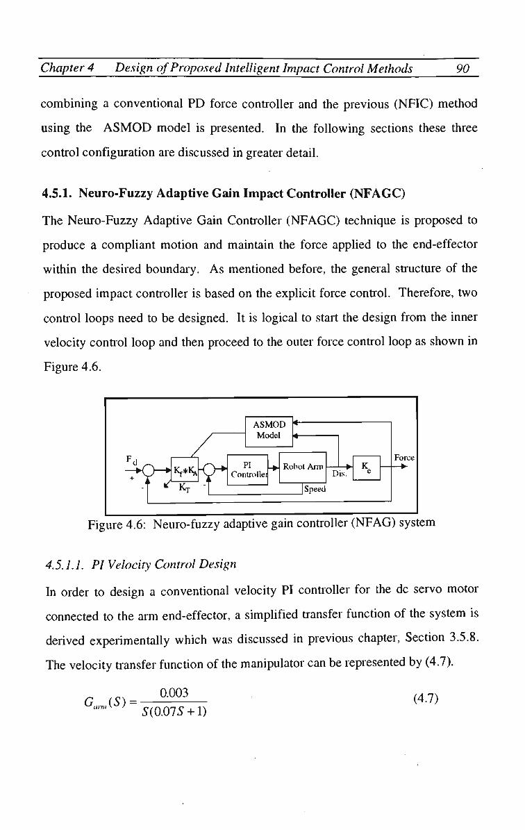
Chapter 4 Design of Proposed Intelligent Impact Control Methods 90
combining a conventional P D force controller and the previous (NFIC) method
using the A S M O D model is presented. In the following sections these three
control configuration are discussed in greater detail.
4.5.1. Neuro-Fuzzy Adaptive Gain Impact Controller ( N F A G C )
The Neuro-Fuzzy Adaptive Gain Controller ( N F A G C ) technique is proposed to
produce a compliant motion and maintain the force applied to the end-effector
within the desired boundary. As mentioned before, the general structure of the
proposed impact controller is based on the explicit force control. Therefore, two
control loops need to be designed. It is logical to start the design from the inner
velocity control loop and then proceed to the outer force control loop as shown in
Figure 4.6.
ASMOD Model
-^CH^ PI
Controllei Robot Arm
Dis. K
Speed
Force
Figure 4.6: Neuro-fuzzy adaptive gain controller (NFAG) system
4.5.1.1. PI Velocity Control Design
In order to design a conventional velocity PI controller for the dc servo motor
connected to the arm end-effector, a simplified transfer function of the system is
derived experimentally which was discussed in previous chapter, Section 3.5.8.
The velocity transfer function of the manipulator can be represented by (4.7).
0.003 G™(S) =
S(0.07S + 1) (4.7)
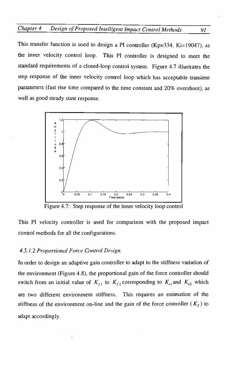
Chapter 4 Design qf Proposed Intelligent Impact Control Methods 91
This transfer function is used to design a PI controller (Kp=334, Ki=19047), as
the inner velocity control loop. This PI controller is designed to meet the
standard requirements of a closed-loop control system. Figure 4.7 illustrates the
step response of the inner velocity control loop which has acceptable transient
parameters (fast rise time compared to the time constant and 2 0 % overshoot), as
well as good steady state response.
1.2 A m
? 1 I I 1 U O.B d e
0.6
0.4
0.2
0
'
0.05 0.1
1 1
0.15 0.2 Time (sees)
—
0.25
'
0.3
>
0.35
-
-
-
0.4
Figure 4.7: Step response of the inner velocity loop control
This PI velocity controller is used for comparison with the proposed impact
control methods for all the configurations.
4.5.1.2 Proportional Force Control Design
In order to design an adaptive gain controller to adapt to the stiffness variation of
the environment (Figure 4.8), the proportional gain of the force controller should
switch from an initial value of Kfl to Kf2 conesponding to Keland Ke2 which
are two different environment stiffness. This requires an estimation of the
stiffness of the environment on-line and the gain of the force controller (KT) to
adapt accordingly.

Chapter 4 Design qf Proposed Intelligent Impact Control Methods 92
•
*___,_
s
K /
Figure 4.8: Gain-Varying Switch Non-linear System
For this purpose, the Adaptive Spline Modelling of Observation Data (ASMOD),
[Kav92] is used.
Given that the ASMOD model can model the non-linear gains accurately, it can
be used as the gain scheduling method in conjunction with the conventional
control. The use of a conventional control algorithm and an A S M O D neuro-
fuzzy system design will reduce the computational burden, and permits analysis
of the performance of the closed-loop system using conventional techniques.
The first step to modelling the total system is to acquire training (input/output)
data and use it to construct the A S M O D model. The training data is produced
while the robot arm is energised by a square wave command to insert the end-
effector into the soil using the experimental rig. The data was obtained by
inserting the end-effector into different types of soil and colliding with different
types of environment, including the body and fuse of A P mines. The contact
force, the travelled distance, and the arm velocity were recorded as the output of
the system during the experiments. As the second step of the modelling task, the
derived data was combined randomly and then divided into two sets of "training"
and "testing" data. Then, the A S M O D algorithm using an iterative method,
builds the model which automatically is adapted to the structure and
dependencies in the data. The best model with minimum enor was finally
chosen. The best model could be selected based on different performance
criteria, such as Root Mean Square enor (RMS), Structural Risk Minimisation

Chapter 4 Design qf Proposed Intelligent Impact Control Methods 93
(SRM), Cross Validation, Akaike's Final Predictor Enor (FPE), Akaike's
Information Criterion (AIC), and the Minimum Description Length ( M D L )
criterion.
The model constructed based on the structural risk minimisation criterion, has a
coefficient vector of 9 coefficients and the structure of the model is presented in
Table 4.1.
Table 4.1: A S M O D model construction for N F A G C .
Sub-model 1
Sub-model 2
Input Variable
l(dx)
2(df)
Intenal knots
3 3
Spline-degree
1 1
As is clear from this Table, this model has two sub-models for displacement and
force derivatives, as input variables. There are also three internal knots for the
linear B-splines (P = 1) in each sub-model. The output of this model is the
stiffness of the environment in contact with the robot arm.
There is another way to represent the A S M O D model, which is the graphical
illustration of the B-spline basis functions for each input variable. Figure 4.9
represents the structure of the constructed A S M O D model given in Table 4.1.
Submodel no. 1 Submodel no. 2
2000 2500
Figure 4.9: A S M O D model to estimate the stiffness of the environment
The output of this model should be applied to the closed-loop force control of the
robot. Before using the adaptive gain controller, a simple proportional gain

Chapter 4 Design qf Proposed Intelligent Impact Control Methods 94
iKf - 0.01) is designed for the robot arm motion in free space. In the process of
designing this gain iKf), it is considered to avoid saturation of the motor
velocity. Without this assumption, the response of the inner velocity control loop
could be easily saturated. This also adds another nonlinear dynamic to the
control system, which should be avoided. W h e n the robot arm is in contact with
an environment with an unknown stiffness, the A S M O D model estimates the
stiffness and then the gain of the controller changes according to the estimated
stiffness.
Kf*^V
•K.T
/
j
ASMuu Model
PI Controllei
-*
4 1
Robot Ann
Speed
Dis." K
Figure 4.10: Neuro-fuzzy adaptive gain controller (NFAG) system
The total gain of the force loop is obtained by multiplying a constant proportional
gain with the adaptive gain KA produced by the A S M O D model.
KT=Kf*KA (4.8)
4.5.1.3. Simulation Scenario
The performance of the N F A G controller is validated through computer
simulation. In the simulation earned out using S I M U L I N K (Figures 4.11 and
4.12), it is assumed that a stiff object, such as an A P mine is located one
centimetre below the ground. The ground is modelled as pure soil with stiffness
of 10 [Kgf/m]. W h e n the arm approaches the mine, the stiffness of the
environment changes suddenly from 10 to the stiffness of the mine.

Chapter 4 Design of Proposed Intelligent Impact Control Methods 95
>p Inptrt
Load Model
Step Inpi
Sum Kf
Kt -•0.01
Ka
Product PI 0.003
0.07S+1
Speed Position
Sumi PID ControllerVransferFcni Sa,ura,ion Transfer F *,! 'Subsystem2
Adaptive Gain A S M O D MODEL
Environment Fs
Subsystem
Figure 4.11: S I M U L I N K graph of the N F A G control system
0.01
mine locat < >i
0.01
mine location
eu Sum
in 1 I r\. Switch 1 out 1
Figure 4.12: Environment model used in the simulation
The stiffness of the mine is assumed to be 2500, 5000 and 7500 [Kgf/m] for three
different cases as illustrated in Figures 4.13 to 4.15. The desired force, which is
the minimum safe force, not detonating the mine, is set to 1 [Kgf]. The
environment is modelled as a switch in which gain changes between two constant
values (Figure 4.12). In each case, the speed of the robot arm and the axial force
are compared with the results of a conventional controller without N F A G .
According to the results, when the end-effector comes into contact with the mine,
the resulting impact force increases suddenly, which is controlled by adjusting the
gain. In the worst case, when the end-effector approaches the mine (stiffness of
7500) from the soil, an overshoot of about 1 0 0 % occurs.

Chapter 4 Design of Proposed Intelligent Impact Control Methods 96
' * 1 1 1 1 i i I i _ 1 5 ~ 25 3 0 US 1 15 2 25
Tim* (M. cor id) Tim» (ttecor.d)
Figure 4.13: Simulation results of N F A G and proportional force when stiffness
changes from 10 to 2500 [Kgf/m]
As can be seen from Figure 4.13, there is no overshoot on the force response of
the system using N F A G , whereas the force response of the system using the
proportional force controller has experienced 2 0 % overshoot. The response of the
N F A G system is 2 0 % slower due to the applied adaptive gain iKA)
conesponding to the stiffness of the first environment with Ke=10 [Kgf/m].
There would have been no slow down in the N F A G response if the robot arm had
approached the stiff environment from free space. This is because the adaptive
gain of the robot arm in free space is equal to one iKA=l). Hence it can be
concluded that the applied adaptive gain control (NFAG) has improved the
performance of the system.
Figure 4.14: Simulation results of N F A G and proportional force when stiffness changes from 10 to 5000 [Kgf/m]
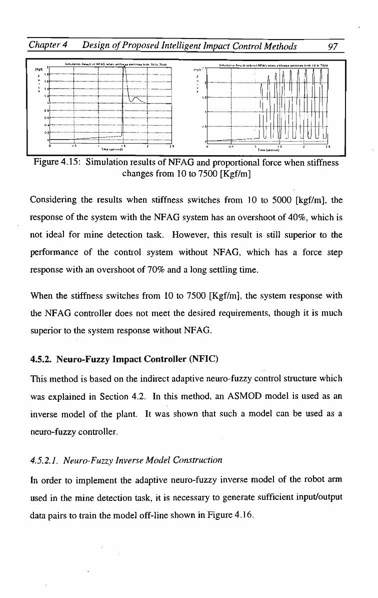
Chapter 4 Design of Proposed Intelligent Impact Control Methods 97
(K9II 2
F " 0 If. r C 1 4
• 1.2
08
06
02
Simulation ft*_uh «l N F A G wii*n ulillr *AMI .Witcti** lorm 10 to 7500
i 1 il\ ! i :
L ' '
! i
: i
i i
' '
1 j
I • 1 i
i
i
j
: i
t
• i
Stmulntior. (Will I wittumt N F A G wl.on _tilli>*bb twitch** lorm 10 lo 7500
_i il u 11 I 0 Tim* (_*coud) Tim* (.ocorid)
Figure 4.15: Simulation results of N F A G and proportional force when stiffness changes from 10 to 7500 [Kgf/m]
Considering the results when stiffness switches from 10 to 5000 [kgf/m], the
response of the system with the N F A G system has an overshoot of 4 0 % , which is
not ideal for mine detection task. However, this result is still superior to the
performance of the conhol system without N F A G , which has a force step
response with an overshoot of 7 0 % and a long settling time.
When the stiffness switches from 10 to 7500 [Kgf/m], the system response with
the N F A G controller does not meet the desired requirements, though it is much
superior to the system response without N F A G .
4.5.2. Neuro-Fuzzy Impact Controller (NFIC)
This method is based on the indirect adaptive neuro-fuzzy conhol structure which
was explained in Section 4.2. In this method, an A S M O D model is used as an
inverse model of the plant. It was shown that such a model can be used as a
neuro-fuzzy controller.
4.5.2.1. Neuro-Fuzzy Inverse Model Construction
In order to implement the adaptive neuro-fuzzy inverse model of the robot arm
used in the mine detection task, it is necessary to generate sufficient input/output
data pairs to train the model off-line shown in Figure 4.16.
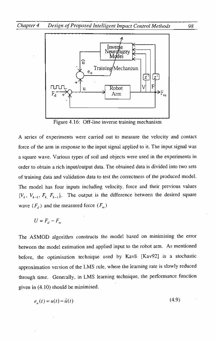
Chapter 4 Design of Proposed Intelligent Impact Control Methods 98
Inverse Neurofuzzy M</del
K-
u
c^ TrainiiwMechanism
rLTLTL
*9 u Robot
Arm
0 V
-»F. in
Figure 4.16: Off-line inverse training mechanism
A series of experiments were carried out to measure the velocity and contact
force of the ami in response to the input signal applied to it. The input signal was
a square wave. Various types of soil and objects were used in the experiments in
order to obtain a rich input/output data. The obtained data is divided into two sets
of training data and validation data to test the conectness of the produced model.
The model has four inputs including velocity, force and their previous values
[Vk, Vk_{, Fk Fk_l]. The output is the difference between the desired square
wave iF(l) and the measured force (F„()
U = Fd-Fm
The ASMOD algorithm constructs the model based on minimising the enor
between the model estimation and applied input to the robot arm. As mentioned
before, the optimisation technique used by Kavli [Kav92] is a stochastic
approximation version of the L M S rule, where the learning rate is slowly reduced
through time. Generally, in L M S learning technique, the performance function
given in (4.10) should be minimised.
euit) = u(t)-u(t) (4.9)

Chapter 4 Design qf Proposed Intelligent Impact Control Methods 99_
J = Eie;it) = ±j^e2uit) = ±-^iuit)-uit))2 (4.10)
The construction of the A S M O D model in this section was terminated at (rmse
=0.1192). The structure of the constructed model which has 34 coefficients is
shown in Table 4.2.
Table *
Sub-model 1 Sub-model 2 Sub-model 3
1.2: A S M O D model construction for NFIC
Input Variable 4 f(k-l)
2 v(k-l)
1 v(k)
3 f(k)
Intenal knots 4
4 4 2
Spline-degree 1 1
1 i 1
This model has two one dimensional sub-models (1 and 2) and one two
dimensional sub-model with Vk and Fk as its input variables. All B-splines basis
functions used in the model are degree one (P=l). The graphical B-spline basis
function representations on the input domain are illustrated in Figures 4.17 and
4.18.
Figure 4.17: Graphical presentation of Sub-model No. 1 and No. 2 of the constructed A S M O D model for NFIC controller

Chapter 4 Design qf Proposed Intelligent Impact Control Methods 100
Submodel no. 3
Var. 3, F(k) -0.04
Var. 1,V(k)
Figure 4.18: Graphical presentation of Sub-model No. 3 of the constructed A S M O D model for NFIC controller
The test data was applied to the constructed model. Figure 4.19 illustrates the
comparison of the model output («) and the input applied to the system (w). In
this figure solid line represents the test data and the dotted line represents the
output estimated by the model. It is obvious that the model is capable of
estimating the dynamics of the robot aim with an acceptable accuracy.

Chapter 4 Design of Proposed Intelligent Impact Control Methods 101_
(Kgf) 1.5
0.5
-0.5
-1
Comparison between model output and system input ~ i 1 1 1 i 1 — - r —
— Test data Output ••• Model Output
>M Wvi i — An
0 100 200 300 400 500 600 700 800 900 1000 Time [msec]
Figure 4.19: Validation of the constructed model for NFIC control
4.5.2.2. Feedforward NFIC without Velocity Controller
The configuration of this control scheme is shown in Figure 4.20. There are two
controllers in this mode. A Feed-Forward Controller (FFC) which is the main
controller and Feed-Back Controller (FBC) which stabilises the closed-loop
system based on the error signal between the desired output signal and the robot
arm output. In this method, the F B C can be either a conventional PID controller
or a neural network controller. In the proposed method F B C is simply a
proportional controller while FFC is designed based on the inverse dynamics of
the robot arm. The input/output mapping of the robot arm will be as follows, if
the feedback control loop is not considered;
y = farmiu) (4.11)
The neuro-fuzzy model estimates the inverse dynamics of the robot arm:
U = fa~rl(y) (4.12)
where f'^ denotes the inverse mapping of fam.

Chapter 4 Design of Proposed Intelligent Impact Control Methods 102
For the reference signal (r), the plant output, which is the outcome of controllers
and the robot arm in series, would be:
> = / « « , ( « ) = /.,«,(/„«('•)) = / (4.13)
This confirms the concept of using an inverse model as the controller, given in
Section 4.4.
NFIC FFC
(V2-* FBC _*£> Robot Arm
Force
Figure 4.20: Block diagram of a NFIC method
Based on the constructed model explained in Section 4.4.2.1 and the proposed
control scheme, a computer simulation using S I M U L I N K was earned out. The
block diagram of the simulated scheme is shown in Figure 4.21. In this
simulation the environment is simulated as a varying stiffness from very soft (10
kgf/m) to very stiff (ke=5000 and 7500 [kgf/m]). The simulation results are
based on the comparison of the step response of the system with and without the
NFIC controller.

Chapter 4 Design of Proposed Intelligent Impact Control Methods 103_
^
NFIC Controller -,
H3—H Delayl
Delay2
uhsygtom Load Model
Step Input $Th$~ 0.003
0.07S+1
Speed 3ositioa
Sum Gainl Servo Motot SaturatiopTransfer Fcn1
Environmen Fs
Subsystem2
Figure 4.21: Simulink graph for feed-forward NFIC
F
r
c
Feedforward NFIC without velocity controller (K» 1-10 and ke2-S000)
! 1 A 1 I | ) v ; ;
___ __J_I____H ] ]
Result witlinui NFIC nnd velocity controller (Kel-10 and ke 2-5000)
I 15 Time (second)
Figure 4.22: Simulation result of feedforward NFIC without velocity control loop when stiffness switches from 10 to 5000 [Kgf/m]
(Kgi)
o
1
•
00
Feedforward NFIC without velocity controller (Kel-10 arid ke2-7P0U)
____]__Z--H
1 !
If i i !
\ \
I NFIC nnd velocity conl poller (Kol-10 «nd k»2-7SOO)
Time (vecond) T.m» (second)
Figure 4.23: Simulation result of feedforward NFIC without velocity control loop when stiffness switches from 10 to 7500 [Kgf/m]
4.5.2.3. Feedforward NFIC with Velocity Controller
In this method, the NFIC controller is used as the explicit force controller, the
same as in the previous method (Section 4.5.2.1), in conjunction with the PI

Chapter 4 Design of Proposed Intelligent Impact Control Methods 104
velocity inner control loop. The proportional gain iKf= 0.01) which was
designed for the N F A G control scheme is also used in this method. By adding
the PI velocity inner control loop, a better performance than the feedforward
NFIC without velocity control is expected.
The simulation scenarios were chosen as before (Section 4.5.1.3) in order to
compare the results. The S I M U L I N K block diagram used for this method is
shown in Figure 4.24. The simulation results are presented in Figures 4.25 to
4.27.
Fd
Step Inpi t
NFIC Controller
*{__§> Delayl Subsystem
<ifc Delay2
Load Model ] Sum2 :£"+ -•0X31>—r>|T
Sum K-I r ^ — •M Cum
PI 0.003
0.07s+1
S >eed
Sum1 Controller Motor
Inner velocity control loop
Saturatior
Environment
Position Subsystem2
Fs
Figure 4.24: S I M U L I N K graph of the NFIC controller with PI velocity controller
SiiM-Mimi A M M * nf NFIC WIMMI riiftiiMt* MMIIJIBS tnttit in In ?&H1 SkmiWinh HHNII* wrlln - il NFIC wtiMi statu HSS switches (otm 10 to 2500
(K.J,
F 1.2-
(K.pO
Tmto (wfctaicj)
l\./.^,L
1.5 -i. Tune (second)
Figure 4.25: Comparison of the simulation results with NFIC and without NFIC when stiffness is switching from 10 to 2500 [Kgf/m]

Chapter 4 Design of Proposed Intelligent Impact Control Methods 105
According to the results obtained for all the three situations, it is obvious that the
performance of the force response deteriorates when the robot arm approaches a
stiff object.
Simvlritinri result ol NFIC WIIPN «Hltot>b!, CIKHIQIH, form 11) to 5UIH.) Sinnilatnii f4.-s.nll witrnml NFIC wtifri .trill.«*& witches lorm 10 to 5000
(Kg I)
1 I
2.„_ 1 i
i Ii i i
j i___J
\
!
Figure 4.26: Comparison of the simulation results with NFIC and without NFIC when stiffness is switching from 10 to 5000 [Kgf/m]
Simulation Ptcwilt ol NFIC when eft Hue** t-wilrl.es ti.rm 10 h- 7«".i 8mnil.itK.fi FtnMili wiilitHii N F A G when .tillnetsB .wilclies lorm 10 lc> 7500
X---1-'
\:lLj\^
j
| {SM]
"" ]_. r__=___-i: u t" W.u.L LMJ t u Time tt->Tc>ii_)
Figure 4.27: Comparison of the simulation results with NFIC and without NFIC when stiffness is switching from 10 to 7500 [Kgf/m]
The result for impact with an object with stiffness of 7500 [Kgf/m] has an
overshoot of 4 0 % , which is acceptable for mine detection. The performance of
the NFIC control scheme is clearly superior to the system response without the
NFIC controller.
4.5.3. Neuro-Fuzzy Impact Control and PID Controller (NFIC/PDPI)
This conhol scheme is based on a combination of NFIC and conventional PID
controller. The NFIC controller will be activated when an impact is detected.
Otherwise the P D force controller is active. The NFIC/PDPI control scheme

Chapter 4 Design of Proposed Intelligent Impact Control Methods 106
which is illustrated in Figure 4.28 is designed based on a neuro-fuzzy ( A S M O D )
inverse dynamic model of the robot arm in contact with the environment.
Fd o^~^ + i i \ /£
. /
P D Force Controller
NFIC Controller tr " L _
Impact
Detector
PI Speed Controller
*
Robot Ann
Speed
Dis. Environment
Force
W
Figure 4.28: NFIC controller block diagram
This conttol method is inspired from the human reflection in collision with an
environment. There is good fusion of force, tactile, sound and vision sensory
systems in a human being to detect a collision and consequently reflect
immediately to minimise possible injuries. In this approach, a fast reaction is
produced by minimising the impact force. The system is stabilised by reducing
the oscillatory behaviour of the conventional impact control methods. A n impact
detector mechanism is designed to add the NFIC control signal to the normal P D
force control system. The impact detector is designed based on the force
derivative to detect a sudden increase/decrease in the force profile and to activate
the NFIC controller when a force threshold is reached. Therefore, it is important
to define a valid threshold to minimise or avoid false detection by the impact
detection mechanism. The minimum value of this threshold could be defined by
the maximum value of the noise present during force measurement. O n the other
hand, the response of the system can become oscillatory if a very low threshold is
selected.

Chapter 4 Design qf Proposed Intelligent Impact Control Methods 107
4.5.3.1. PD Force Control Design
In order to design an explicit force controller, the robot arm with the previously
designed PI velocity controller as its inner loop is considered. A P D force
controller which is a good candidate for an explicit force controller [Vol91] is
designed to stabilise the system response. The root locus of the whole system,
before and after introducing the P D force controller is shown in Figure 4.29. It is
clear that the system response without P D force controller is unstable for gains
more than one.
I H K > [ i i ' r
•100 -80 -BO -411 -M ' 4 0 HI M '***«> -150 -««> -SO 0 50 100 ISO 200 FlnalA^ R_IA*i
Figure 4.29: Root locus for the total system.
The stabilised system will have a faster step response if the zero of the PD is
located in the most far left of the real axis. Figure 4.30 illustrates the step
response for the designed P D force controller (Kp=0.01 Kd=0.0001) which has a
zero atz=-100.
11 • i
,,N [____]

Chapter 4 Design of Proposed Intelligent Impact Control Methods 108
Figure 4.30: Step response of the PDPI explicit controller for the P D force controller
This Figure illustrates the force step response of the PDPI controller when the
robot arm comes into contact with two different types of environment iKel=50
and Ke2=5000). As is clear the P D should be designed to produce an acceptable
step response for a wide range of stiffness. If it is desirable to have a faster
response when the robot arm is in contact with a soft environment, the P D
controller can be designed ieg. Kp=0.3 Kd-0.0001) to have a settling time of less
than one second.
Figure 4.31: Step response of the PDPI explicit force controller
Figure 4.31 illustrates the step response of the new PDPI (PD force and PI
velocity) controller for two different types of environment (Kel=50 and
Ke2-5000). The system is unstable for the suffer environment. Therefore, it is
necessary to find a trade off between stability of the system when in contact with

Chapter 4 Design qf Proposed Intelligent Impact Control Methods 109
a stiff environment and the speed of the response when in contact with a soft
environment or in free space.
4.4.3.2. Simulation Results of the NFIC/PD Control Scheme
In this section two versions of the new control scheme are simulated. The first
version is a combination of NFIC and a P D force control without using the PI
velocity control (NFIC/PD) while the second version includes the PI velocity
conhol (NFIC/PDPI). Figure 4.32 illustrates the S I M U L I N K block diagram of
the NFIC/PD method. Impact detection control which receives the measured
force and its previous value, detects a sudden change in the induced force. A
sudden change in force profile could be due to transition from free space to a stiff
environment or just caused by noise. In the following simulation results, the
threshold value for the impact detection is set to 0.2 [Kg], which is more than the
noise level observed in a physical system.
Fd
ED Step
^
•>!_____—•
NFIC Controller
Delay2
Delayl Subsystem
->r—' PID
Sum PD
Load Model ]
c,,m.i Gainl
0.003 0.07S+1
5peec Position
Environment
Motor Saturation |ntegrator l - — - ^
Wf__Z]-Deiay3
Impact Dete
Subsystem3
Fs
Constant 1
Figure 4.32: S I M U L I N K graph of the NFIC/PD control system
The simulation results for the NFIC/PD control are illustrated in Figures 4.33 and
4.34. According to these results, which are compared individually with the P D
force control without NFIC control, there is a quite robust force response to
variations in the environment stiffness. The conventional controller has shown a
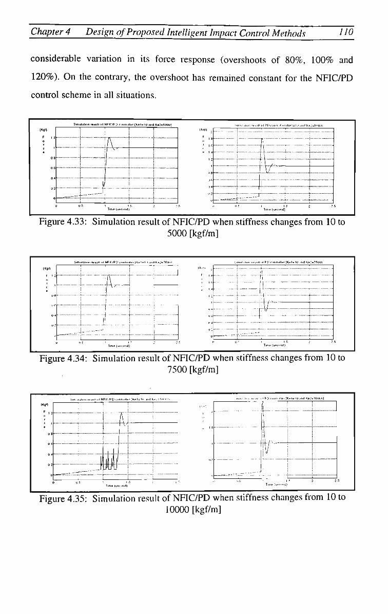
Chapter 4 Design qf Proposed Intelligent Impact Control Methods 110
considerable variation in its force response (overshoots of 80%, 100% and
120%). On the contrary, the overshoot has remained constant for the NFIC/PD
conhol scheme in all situations.
StmulnitoTi t-wilt i>t NFK:/F'[i ci-MnJIf i {K»1 = 10 tirid K » 2 c 5 0 W )
1*90 .1 F'[) (irf.inJlHi (Kol-Ui and Ke.'=SWO)
Time (_4tri>hd)
Figure 4.33: Simulation result of NFIC/PD when stiffness changes from 10 to 5000 [kgf/m]
SMnidnlinti ir_ul1 of NFtdJ'Ei r<-ili<>llei (K^l-lii ;,r.rl K»2-7f.i
(Kgt)
"* '
J -
Mn...l -, .--.I ..1 f[ic<..iuJli.( ( K H 1 = K » n.d K*-?=7SUUt
! ; ' ' i f ! . 1
j -J
1 : ; ft • !
.1 ! : • ; ! ;|/ ; . v ; j
; . ; ;
Figure 4.34: Simulation result of NFIC/PD when stiffness changes from 10 to 7500 [kgf/m]
I ('[i n.iiliollcf (K(-1 = Uiiiiid K* 2= 10000)
Tim*. |t>ftitid) TKNt. (•>-(.«.(])
Figure 4.35: Simulation result of NFIC/PD when stiffness changes from 10 to 10000 [kgf/m]

Chapter 4 Design of Proposed Intelligent Impact Control Methods 111
The oscillation is due to the adaptation mechanism which sometimes takes too
long and hence introduces some noise into the system performance.
4.4.3.3. Simulation Results of the NFIC/PDPI Control Scheme
In order to see the effects of the designed PI velocity controller as the inner
control loop and investigate the performance of the NFIC/PDPI control scheme,
in this section the PI velocity controller is added to the control method presented
in the previous section. The simulation block diagram is given in Figure 4.36.
The NFIC controller is activated when a sudden change in the measured force is
detected. The threshold level for impact detection is set to 0.2 [Kg]. Simulation
results for the three different situations when the environment stiffness varies
from 10 to 5000, 7500 and 10000 [Kgf/m], compared with the system with no
NFIC controller, are illustrated in Figures 4.37 to 4.39. Again, it is quite clear
that in each situation, results of NFIC/PDPI control scheme give a better
performance than the PDPI controller without NFIC.
r4d
U Step
^
NFIC Controller —,
>{____}-H Delay 1 Subsystem
— K T i
Delay2
Load Model
PID
Sum PD PID
0.003
0.07S+1 Sum3 Sum1 PI Motor
Saturation
*__§_]-Delay3
Impact Dete.
Speej Posi,i,p
_&-prHE illiration § I I —
Environment —*i
Transfer Fcn$ubsystem2
.Subsystems
0 Constant 1
Figure 4.36: S I M U L I N K graph of the NFIC/PDPI control system
In the NFIC/PDPI control scheme, there are some oscillations in the response
after impact detection. But in all situations, the overshoot does not go above 2 0 % ,
regardless of the environment stiffness.

Chapter 4 Design of Proposed Intelligent Impact Control Methods 112
Simulation mull PI NFIC/PDPI controller (K.lglQ and k«2«50001
[Kgi]
SimulalKHi i»_utl ol PDPI «mUoll»( {K«1=10 and k»2=SOO0]
Tim* (wcond) Tim* (wcond)
Figure 4.37: Simulation result of NFIC/PDPI and PDPI when stiffness changes from 10 to 5000 [kgf/m]
Simulation result ol NFlOVPDPI controller (K»1 = 10 and k_2=75(K>)
4 - 4 4 j i j
[Kgn 1 8
» 1.2
U8
Simulation result ol PDPI c rmlrollar (Ke1=10 and ke2=7500)
i A i
I )•••
I I-
I — f -
|M—H j i
I r . i
Figure 4.38: Simulation result of NFIC/PDPI and PDPI when stiffness changes from 10 to 7500 [kgf/m]
Simulation result ol NFIC/PDPI controller {Ke1=1U find ke2=100W)
(Kgl)
Time (»ec(rnd)
(Kql) 1 8
F
Simulalion rpsuli el PDPI controller (K*1=10 and ke2=i0OO0)
c
0
1 r- — •• I . , ,.,
| \ \ |
1 ;....
_™»=n.-4:-.--r;.....:4:..
, A |
t [ A / 1 A -III/
i 1
Time (second)
Figure 4.39: Simulation result of NFIC/PDPI and PDPI when stiffness changes from 10 to 10000 [kgf/m]
4.6. Conclusion
In this chapter the design procedure and simulation results for three intelligent
impact control schemes have been presented. A neuro-fuzzy adaptive gain
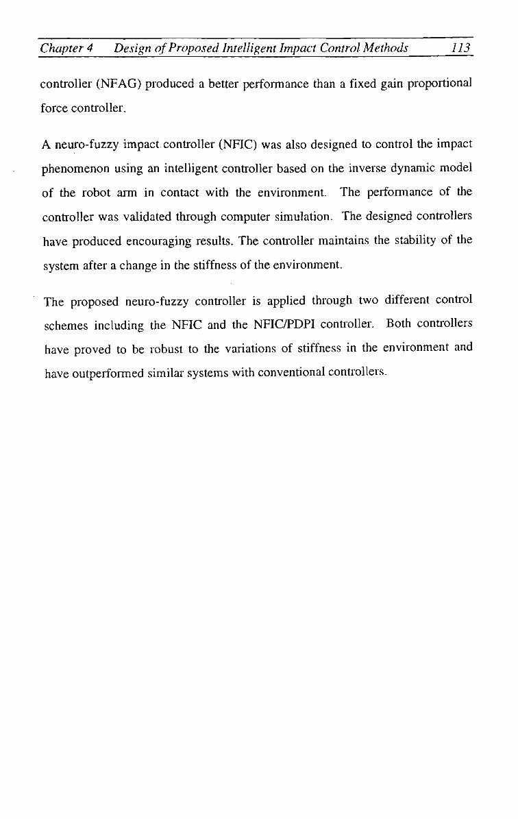
Chapter 4 Design of Proposed Intelligent Impact Control Methods 113
controller ( N F A G ) produced a better performance than a fixed gain proportional
force controller.
A neuro-fuzzy impact controller (NFIC) was also designed to control the impact
phenomenon using an intelligent controller based on the inverse dynamic model
of the robot arm in contact with the environment. The performance of the
controller was validated through computer simulation. The designed controllers
have produced encouraging results. The controller maintains the stability of the
system after a change in the stiffness of the environment.
The proposed neuro-fuzzy controller is applied through two different control
schemes including the NFIC and the NFIC/PDPI controller. Both controllers
have proved to be robust to the variations of stiffness in the environment and
have outperformed similar systems with conventional controllers.

Chapter 4 Design of Proposed Intelligent Impact Control Methods 114
Ke varies from 10 tO 5000
(D
(2a)
(2b)
IKot) !
Simulation Re.utl ol N F A G whan fltflnais iwrlohai la m tO lo SOCIO
! f
_ i — ^ — '
•--- -
• ! - — -
flerweid NFIC without velocity controller (Kei-io end ke2-6000]
• —
- ----
;
(\ : v
1
Sunulaliei, itsuK ol NFIC oil •n (litlnass chanoag tori ID lo 6000
i
i
A IW Hyp y
1 i
---~~---q___f----
Simulation ra.ult ol NFIC/F'O conliollar (Kol-10 end KoZ-SOOO)
(3a)
Simulation raiuH ol NFHJ/PD^IconHollar (,Ket-tO and hog-SOOQ)
!
I \i 1 1 •
1 !
1 •ll/ 1 •
__ 1 ;
i •
(3b) 1 If.. » I • • < '.!•« '
Ke varies from 10 tO 7500
Minuliiu.n fcaiull ol N F A G whan stillnaai rwitctiee lorm 10 to 7600
IKgl)
F t :
T" : d
(Kg')
.
0
Faadloiward NFli: trill • ulv«
—.,^7-h:.::-:;::r T_....
ociiy controller (Kol.to ond koZ-75O0)
I [
1 | \T~
i
i
i-
Tr.na(socond)
.-. - F-.c mt ol NFli: when stillness switches term tOlo 7fi00
i
f '1 P : ;
Time (fecond]
..,.,1,1,.... result ol NFIUff'D controller (Kel-10 end Ke_-76001
Time (second]
.SHIM Mi or, re:ull ol NF icff'Of'i contro
\l
Am ™._iLnl
! .
tar (K*I*10 andke£-7600)
i A
\j-\/^^-T-
'.
Figure 4.40: Force response comparison of all the proposed methods

VALIDATION OF CONTROL
STRATEGIES

Chapter 5 Validation of Control Strategies 116
5.1. Introduction
In this chapter the experimental work conducted to validate the proposed
intelligent control system is described. Initially, the structure and details of the
experimental rig will be explained. This experimental rig is the same as the one
used in Chapter 4 to validate the simulation results. Afterwards some hardware
and software problems encountered during the implementation of the demining
robot will be discussed. The experimental results of the intelligent impact control
methods are compared with the conventional impact control schemes to illustrate
the validity of the developed system. The obtained results will be finally analysed
and some concluding remarks will be made.
5.2. Experimental Rig
At this stage the work is focused on a single axis force controlled arm to drive the
bayonet as its end-effector. The robotic aim imitates the operation of a human
de-miner using the hand prodding approach. As shown in Figure 5.1, the device
consists of a bayonet which is attached to a dc servo motor (Hitachi) via a load
cell (force sensor) and a linear distance sensor (Linear Variable Differential
Transformer-LVDT) to measure the linear translation. As the bayonet is inserted
into the soil, the generated reaction force is measured by the force sensor.
A normal bolt and a long screw, assembled as a lead-screw mechanism with a
considerable amount of backlash and static friction, is used to convert the rotation
of the motor to a linear translation. The arm is assembled with a 30 degree angle
to the ground to induce half (sin(30°)xFv) of the axial force to the object in
contact with the bayonet. In the following sections, specifications for the dc-
servo motor and sensors are given in more detail.

Chapter 5 Validation of Control Strategies 117
Figure 5.1: End-effector connected to the force and L V D T sensor
5.2.1. D C Servo Motor Specifications
The specification of the Hitachi dc servo motor, including the rotational speed
transducer which is used to drive the end-effector of deminer arm, is given in
Table 5.1.
Table 5.1: Hitachi D C servo motor specifications
Input Voltage Current Max. Speed Torque Output Power Pulse/Rotation
24 [VDC] 2.2 [A] 1880 [RPM] 0.212 [Nm] 33 [W] 640
The accompanying rotational speed transducer is an incremental shaft encoder
which simply uses one set of opto-electrical sensors. The incremental shaft
encoder consists of a disc in which a series of holes or marks are engraved
around the periphery. A light source, usually a light emitting diode, is positioned
on one side of the disc and a photosensitive transistor on the other. Rotation of
the disc generates a series of light pulses which are registered as a square pulse

Chapter 5 Validation qf Control Strategies 118
train output from the photosensitive transistor. By using a mechanism consisting
of two light sources, the direction of the rotation can be detected. This is not
included in the Hitachi dc servo motor. Therefore, alternatively, the applied
voltage to the motor or current taken by the motor is measured to identify the
direction of motor rotation. The output waveform, which is a train of pulses, is
counted over a constant period of time to convert the number of pulses to
rotational speed of the motor.
5.2.2. Load Cell Specifications
The force sensor used in the experimental rig is a load cell with specifications as
given in Table 5.2.
Table 5.2: Load cell Specification
Model Rated Load Output Voltage Non-linearity
XTRAN-K4 25 Newton 2.843 mV/V at rated load ! +/-0.01%
Load cells which are normally used as force, pressure, or torque transducers are
based on a strain measurement, which is essentially a displacement. The physical
variable to be measured ultimately causes, by design, a deflection in an elastic
member. Direct measurement of the strain associated with the deflection can
then be related back to the physical variable through calibration. Strain sensitive
sensors are incorporated into a Wheatstone bridge circuit.
The Wheatstone bridge consists of four resistors, a voltage source and usually a
high impedance instrument to record the bridge output voltage. W h e n the bridge
is balanced, no current is drawn through the voltmeter. The sensing element,
which is normally a strain gauge, constitutes one arm of the bridge while the
other three anus have constant resistance equal to the sensing element at no load

Chapter 5 Validation of Control Strategies 119
condition. The bridge normally operates in an unbalanced mode where the
voltmeter reading is used to quantify the changing conditions at the sensing
element, which is the result of changes in the measured physical variable. Figure
5.2 shows a normal bridge configuration in unbalanced mode.
Figure 5.2: Unbalanced mode Wheatstone bridge
It is assumed that the bridge is initially in balance, with all elements having a
resistance R. The sensing element is then subjected to a condition which causes
its resistance to change to (R + AR). The bridge thus becomes unbalanced and a
potential difference v is generated and registered on the voltmeter. Given that the
voltmeter has nearly infinite resistance, there will be a zero current drawn
through the voltmeter. The current drawn through A and C is V/2R, while that
through B and D is V/ilR + AR). The potential seen at x will be:
(V - RV/2R) = V/2
The potential seen at y is;
V-ViR + AR)/(2R + AR)
The resultant potential difference (x-y) is:

Chapter 5 Validation of Control Strategies 120
_V AR 1 V ~ 2 R i2 + AR/R)
If R))AR, the potential difference is given approximately by:
VAR
Equation (5.1) gives a linear relation between the potential difference v and the
changes in the strain gauge resistance AR, which is the only variable in the
equation. It should be noted that an instrumentation amplifier, including a
differential amplifier with high input impedance, should be used to avoid loading
the bridge. In the experimental rig, an off-the-shelf strain gauge amplifier with
the given specifications (Table 5.3) is used to amplify the potential difference v.
Table 5.3: Instrumentation amplifier specifications
Supply Voltage Input offset voltage Input offset voltage/supply
Input impedance Input noise voltage
Band width (unity gain) Output current Common mode rejection ratio Maximum bridge supply current Power dissipation
+1-2 to +/-20 V dc 1 1 m V max 5p:V/V
>2.5MQmin 1 |j,Vp.pmax
400 kHz 5 mA > 100 dB 12 mA 0.5 W
5.2.3. Linear Variable Differential Transformer (LVDT)
The L V D T is widely used as a measurement and control sensor wherever
displacements of a few micro-inches to several feet need to be measured directly.
Such a sensor also can be used to measure other physical quantities, such as force
and pressure, after being converted to linear displacement. The L V D T is
extremely accurate, can operate in extreme conditions and produce repeatable
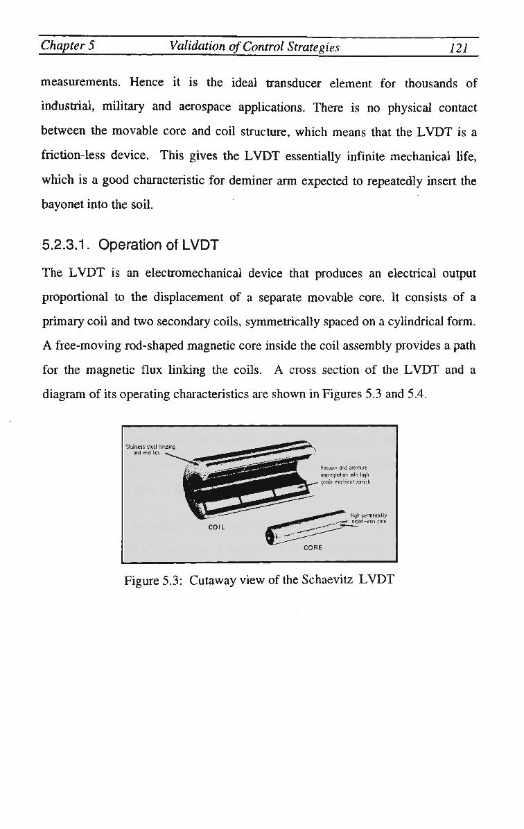
Chapter 5 Validation of Control Strategies 121
measurements. Hence it is the ideal transducer element for thousands of
industrial, military and aerospace applications. There is no physical contact
between the movable core and coil structure, which means that the L V D T is a
friction-less device. This gives the L V D T essentially infinite mechanical life,
which is a good characteristic for deminer arm expected to repeatedly insert the
bayonet into the soil.
5.2.3.1. Operation of LVDT
The L V D T is an electromechanical device that produces an electrical output
proportional to the displacement of a separate movable core. It consists of a
primary coil and two secondary coils, symmetrically spaced on a cylindrical form.
A free-moving rod-shaped magnetic core inside the coil assembly provides a path
for the magnetic flux linking the coils. A cross section of the L V D T and a
diagram of its operating characteristics are shown in Figures 5.3 and 5.4.
jtumless .ttf.l housing arid end lids
COIL
Vacuum and pressure
impregnation with high grade electrical varnish
High permeability ,., -ri' nickel-iron core
CORE
Figure 5.3: Cutaway view of the Schaevitz L V D T
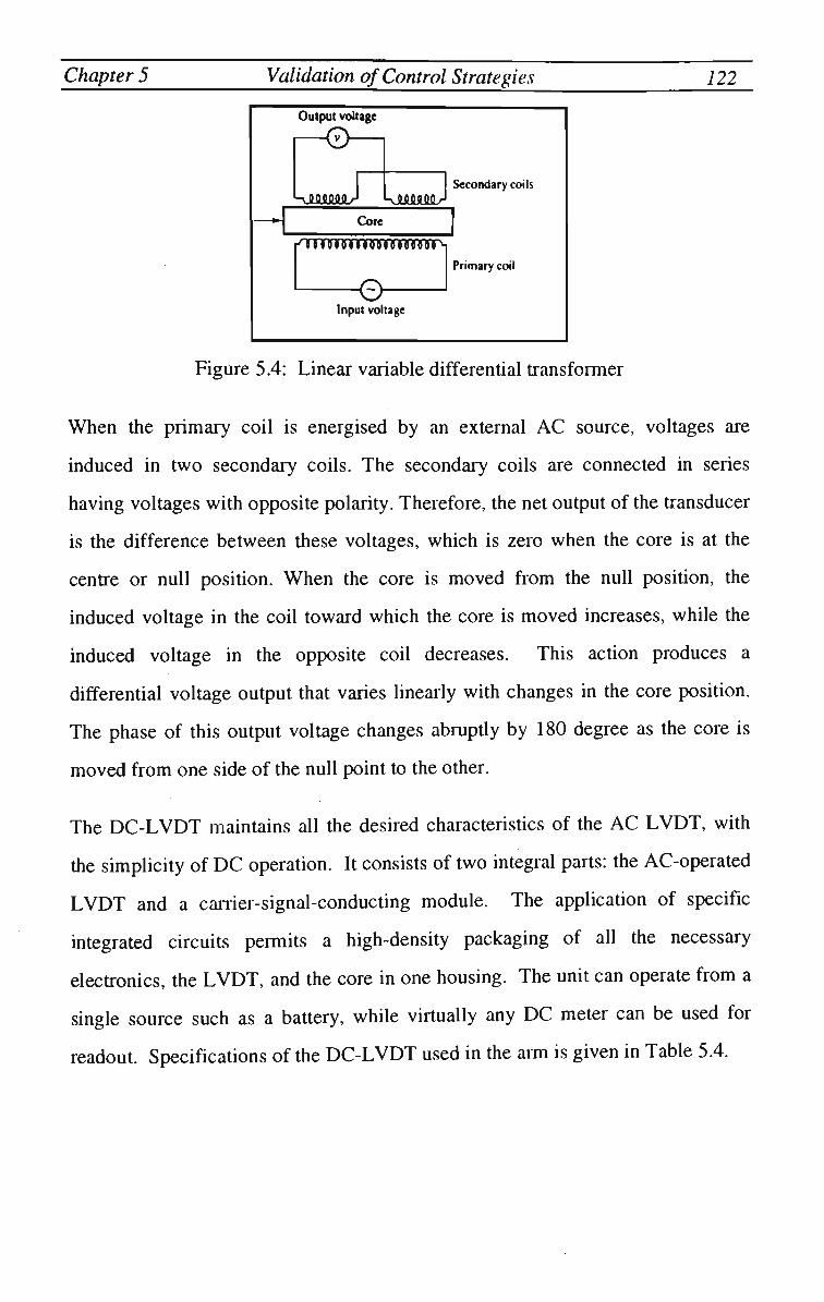
Chapter 5 Validation of Control Strategies 122
Output voltage
•Cyj •
kjlflJUlfiJLr -vMUJUL/-Core
rarnrrini'JOTnin mm mm \
Input voltage
Secondary coils
Primary coil
Figure 5.4: Linear variable differential transformer
When the primary coil is energised by an external AC source, voltages are
induced in two secondary coils. The secondary coils are connected in series
having voltages with opposite polarity. Therefore, the net output of the transducer
is the difference between these voltages, which is zero when the core is at the
centre or null position. W h e n the core is moved from the null position, the
induced voltage in the coil toward which the core is moved increases, while the
induced voltage in the opposite coil decreases. This action produces a
differential voltage output that varies linearly with changes in the core position.
The phase of this output voltage changes abruptly by 180 degree as the core is
moved from one side of the null point to the other.
The D C - L V D T maintains all the desired characteristics of the A C L V D T , with
the simplicity of D C operation. It consists of two integral parts: the AC-operated
L V D T and a carrier-signal-conducting module. The application of specific
integrated circuits permits a high-density packaging of all the necessary
electronics, the L V D T , and the core in one housing. The unit can operate from a
single source such as a battery, while virtually any D C meter can be used for
readout. Specifications of the D C - L V D T used in the arm is given in Table 5.4.
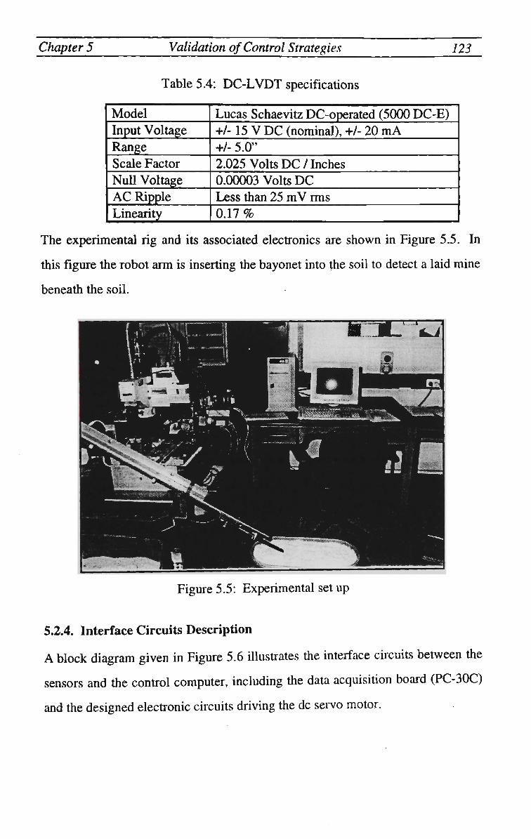
Chapter 5 Validation of Control Strategies 123
Table 5.4: D C - L V D T specifications
Model Input Voltage Range Scale Factor Null Voltage A C Ripple Linearity
Lucas Schaevitz DC-operated (5000 DC-E) +/-15 V D C (nominal), +/- 20 m A +/- 5.0" 2.025 Volts D C / Inches 0.00003 Volts D C Less than 25 m V rms 0.17 %
The experimental rig and its associated electronics are shown in Figure 5.5. In
this figure the robot arm is inserting the bayonet into the soil to detect a laid mine
beneath the soil.
Figure 5.5: Experimental set up
5.2.4. Interface Circuits Description
A block diagram given in Figure 5.6 illustrates the interface circuits between the
sensors and the control computer, including the data acquisition board (PC-30C)
and the designed electronic circuits driving the dc servo motor.

Chapter 5 Validation of Control Strategies 124
r__3
oojtr 1200 _Hr
Pentium
j
< '
Data Acquisition PC30C
l
D C Motor PWM/Driver
> D C Servo Motor +
End-effector
t
r -\ Electronic Circuits Interface
M
Shaft Encoder
I\I\
Sensor
' 1 0 LVDT 7
Bayonet i
Figure 5.6: Hardware configuration of deminer arm
The interface card PC-30C supports 16 analog input channels with a 100 kHz
A/D converter, 24 digital I/O lines and four D/A converters connected to the
analog output channels. The interface components include the force sensor
amplifier, P W M servo motor driver, and a digital circuit measuring the speed of
the motor by counting the pulses from the shaft encoder.
5.3. Commissioning of the Experimental Rig
There were a number of difficult problems encountered during commissioning of
the hardware and software of the experimental rig.
5.3.1. Hardware Problems
As the constructed experimental rig was the first prototype deminer robotics arm
developed at Wollongong, a number of problems regarding the mechanical
design and manufacturing inaccuracies were encountered. Some examples were
varying friction of the mechanism according to the position of the end-effector,
backlash and vibration of the arm. In the mechanical structure of the deminer, a
normal bolt and a long screw are assembled as a lead-screw mechanism with
considerable amount of backlash. On the other hand the screw which is

Chapter 5 Validation qf Control Strategies 125
connected to the end-effector, is off-centred relative to the motor shaft. Hence, a
considerable amount of static friction, which varies according to the position of
the bolt, affects the performance of the control system. Impact control can
perform satisfactory when the system has an accurate positioning mechanism
with no backlash. The backlash involved with the experimental rig, is quite high
and can significantly deteriorate the performance of the impact controller. For
this reason and because of the noise involved with the force sensor, the step
response of the deminer sometimes demonstrates another transient response after
reaching a steady state.
The experimental results clearly show a considerable amount of unwanted noise
in the force signal, which is due to the vibration of the arm when the bayonet is
inserted into the soil. Another problem encountered is the unpredictable and
variable static friction which effects the steady state enor of the system.
5.3.2. Software Problems
The major software problem encountered in this thesis was the conversion of
M A T L A B M files to C programming language running in a D O S environment.
The A S M O D algorithm employed in this work, was initially developed by T o m
Kavli [Kav92] in a M A T L A B environment. There was no problem in using M
files in off-line training as time was not so critical. However, they are too slow
for on line estimation of the model. They needed to be converted to a more
efficient programming language. Since the data acquisition software was written
in C, it was decided to convert the A S M O D M files to C.
At the first attempt, the converter toolbox provided by M A T L A B was used. The
code produced by this toolbox runs only in the Microsoft Windows environment
[Mat96a] which is not very efficient due to the operating system overheads. The
second package used to convert the M files was a C + + compiler D J G P P

Chapter 5 Validation qf Control Strategies 126
supported by M A T C O M [Mat96b] for the D O S environment. This converter
proved quite successful and the generated code ran on D O S with no problem. As
this compiler was not supported by the data acquisition board (PC30) library, all
the drivers for the board had to be modified for the D J G P P compiler.
The generated code produced an execution time of 10 [msec] for each iteration of
the program without updating the A S M O D model on a Pentium 200MHz. But
when it was attempted to update the A S M O D model on-line, the execution time
for each loop increased to about 50 [msec], which is five times more than the
sampling period (T=10 [msec]) used in the digital controller.
Therefore, it was decided to update the A S M O D model only after one complete
procedure of probe insertion by the collected input/output data rather than
updating the A S M O D model on-line. It was, however, realised that there was no
considerable difference between the updated model and the original one. The
reason was that in consUuction of the model, different types of soil were taken
into account.
5.3.3. Implementation of Digital PID Controller
Digital P (proportional), PI (proportional + integral) and P D (proportional +
derivative) controllers were used in conjunction with the intelligent controllers in
the experimental work. The sampling time used for the digital controllers was
the same as the sampling time used in the S I M U L I N K simulation (T = 0.01
Seconds). The following algorithm was used to implement the digital PID
controllers:
w_*,+M(i±l)+£fci=!, 2 z-1 T z

Chapter 5 Validation of Control Strategies 127
where KP, Kj and KD are the controller and T is the sampling period of the digital
control loop. Comparing the above PID controller structure with the standard
form of a second order pulse transfer function
a0+aiZ_ 1 + a2z~
2
Diz)= l + b}z~
l+b,z
the parameters will be obtained as follows:
a, = KP+^KtT + jKD
ai=-KP+±K}T-jKD />,=-l
a2=~KD b2=0
In order to obtain an execution time for each loop of the digital controller equal
to the selected sampling time, a special C + + function provided with the D J G P P
compiler was used. Using this function, it was possible to measure the execution
time in microseconds. The difference between the sampling time and the
execution time can then be delayed sufficiently to produce the desired sampling
time for each loop of the program.
5.4. Validation
In order to validate the proposed impact control methods described in Chapter 4,
a series of experiments were conducted to locate a VS-50 A P mine laid under the
garden soil. For each control method, three different sets of results based on the
variation of the garden soil (environment) are presented. This was achieved by
mixing the garden soil with other ingredients such as sand, clay, and small stones.
Moreover, the soil which was used for the first set of results (labelled 'A') was
dried loose soil, while for the second set of results (labelled 'B') it was the same

Chapter 5 Validation of Control Strategies 128
but compressed and for the third set of results, water was added to provide a
different environment. The experimental results for each control method has
been presented in the same order as the simulation results presented in Chapter 4.
In order to illustrate the effectiveness of the intelligent controllers, their
performances have been compared against a system using a conventional
controller.
The results of the experimental work are given by a set of diagrams which
illustrate the measured force during the insertion of the robot arm into the soil
and the impact stage when the arm has reached the body of an A P mine. In each
diagram, the results with the intelligent methods are shown in black lines while
the results with pure conventional controllers are in faded black.
5.4.1. Neruo-Fuzzy Adaptive Gain (NFAG) Controller
The N F A G technique based on the adaptive gain (Section 4.5.1) was
implemented in real time using a P C Pentium 200MHz. Figures 5.7, 5.8 and 5.9
compare the performance of the N F A G algorithm against a proportional force
controller. The PI velocity controller is the same as the one presented in Chapter
4, Section 4.5.1.1. The arm becomes stationary when it comes into contact with a
stiff environment. Accordingly, the resulting static friction causes some
problems such as steady state error or stick/slip phenomena.

Chapter 5
2.5
To. __ ® 1.5
8 u.
0.5
Validation of Control Strategies
Practical Result ol N F A G controller
™
ii UjaJ
•
rn.
1 1 1 i ! !
With NFAG
Without NFAG
r~
j i
;
—
j
j
^FT?f fflSF'^f^F' roi " r" vIP Tin"" ™f 7
1 ! L.
T "f' IT ! 1
6 8 10 12 Time[s]
14 16 18 20
Figure 5.7: Experimental result of N F A G Controller (A)
129
Practical Result ol N F A G controller
2.5
® 1.5 o LL
0.5
i J Jl AM ll
j
\l
| I f j I
i i I i
> _ - • »
}-,
I j j
With NFAG
Without NFAG —
r"'" •
w||# rfTt j__kniM«_J_y4
l
e 10 12 Time[s]
14 16 18 20
Figure 5.8: Experimental result of N F A G Controller (B)
Figures 5.7, 5.8 and 5.9 clearly illustrate that the NFAG control method produces
a better performance than the conventional proportional controller. One of the
most significant differences is the overshoot percentage of the fixed proportional
controller which is about 300%.

Chapter 5 Validation of Control Strategies 130
3.5
2.5
s a* 1.5
0.5
-0.5
Practical Result ol N F A G controller
Uk&to* S f c f c * * ^
1. 1
1 1 1
I :
With NFAG
Without NFAG
m^WBmmmsam I'tfn
V
JEL^L." ,TIH \nVf n » ilMI'P
4 6 8 10 Time[s]
12 14 16
Figure 5.9: Experimental result of N F A G Controller (C )
Overall the NFAG algorithm produced a smoother response and a smaller
overshoot compared to the conventional controller which had an oscillatory
response. The slower response of the N F A G algorithm was its only shortcoming,
which was also obvious in computer simulation. The slow response is due to the
inverse dependence of the adaptive gain, KA generated by the neuro-fuzzy
model, on the environment stiffness. Hence, the total gain of the control loop is
smaller than the gain of the fixed proportional controller. This was the case only
when the arm was in contact with the environment, whereas the response of the
arm in free space motion is the same as the fixed proportional controller.
5.4.2. Neuro-Fuzzy Impact Controller (NFIC)
As explained in Chapter 4, Section 4.5.2, this method was based on an indirect
adaptive neuro-fuzzy control structure in which the derived A S M O D model is
used as an inverse model of the plant.

Chapter 5 Validation of Control Strategies 131
5.4.2.1. Feedforward N F I C with PI Velocity Controller
The control block diagram for this control method is presented in Chapter 4,
Section 4.5.2.2. The experimental results for three different situations based on
the soil variation (dry (A), dry compact (B) and wet (C)) are given in Figures 5.10
,5.11 and 5.12. From these figures, it can be seen that the performance of the
impact controller with NFIC is superior to the system without the NFIC
controller. The overshoot for the NFIC controller has a maximum value of 2 0 %
compared to 2 5 0 % overshoot for the controller without NFIC.
Practical Result o( feedforward NFIC with PI Velocity controller
I
!
i
1 1 w rn
W*fH V f
+~""T '
\
1 li W
- j
With NFIC
Without NFIC
I
i i ... . A i I I 1 1 1- 1 '
0 2 4 6 8 10 12 14 16 Tlme[s]
Figure 5.10: Experimental result of feedforward NFIC with PI velocity control
loop (A)
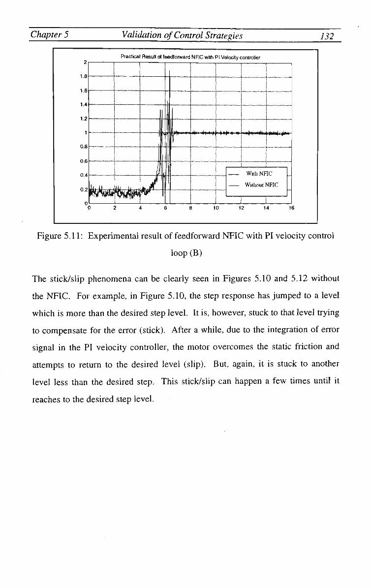
Chapter 5 Validation of Control Strategies 132
Practical Result ol leedlorward NFIC with PI Velocity controller
U*-U nHA
rfP Ik 4A..+.I
Ul TT ru ]\T '
j AjirT
flr 1
I ~*
f
• " '
i»fc*n»i^M
With NFIC
Without N F I C
i i
0 2 4 6 8 10 12 14 16
Figure 5.11: Experimental result of feedforward NFIC with PI velocity control
loop (B)
The stick/slip phenomena can be clearly seen in Figures 5.10 and 5.12 without
the NFIC. For example, in Figure 5.10, the step response has jumped to a level
which is more than the desired step level. It is, however, stuck to that level trying
to compensate for the error (stick). After a while, due to the integration of error
signal in the PI velocity controller, the motor overcomes the static friction and
attempts to return to the desired level (slip). But, again, it is stuck to another
level less than the desired step. This stick/slip can happen a few times until it
reaches to the desired step level.

Chapter 5 Validation of Control Strategies 133
Practical Result ol leedlorward NFIC with PI Velocity controller
1 :
With NFIC
Without NFIC
lijAt lAAl i-U*.--ti-M
|ii- (> #
m^l ll( ft
rH
r
M
w
frW;.*».-...-i-
ffi
0 2 4 6 8 10 12 14 16
Figure 5.12: Experimental result of feedforward NFIC with PI velocity control
loop ( C )
It is also clear that the performance of the control system without the NFIC
controller is very poor. This is contrary to the results produced in the computer
simulation (Figures 4.25 to 4.27). The reason for this difference between the
practical and simulation results could be the effect of non-linearities such as
backlash, and friction not taken into account in the conventional controller and
also the noise produced by the force sensor and other elements of the system.
5.4.2.2. Feedforward NFIC without Velocity Controller
In order to implement this control method the same block diagram given in
Figure 4.21 is used. The experimental results are also based on the comparison
of the step response of the system with NFIC against the system without it.
Figures 5.13, 5.14 and 5.15 illustrate the results of the NFIC impact controller
without the velocity conhol loop.
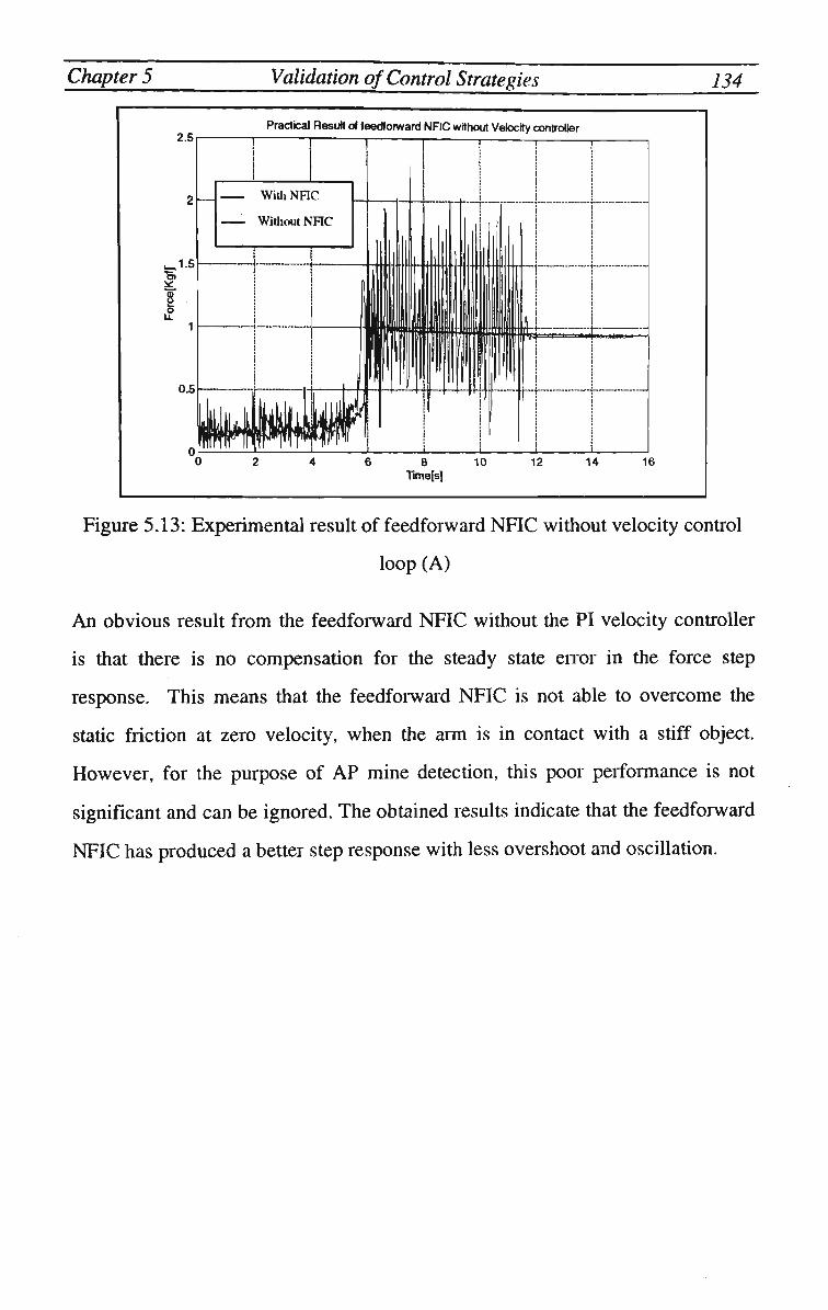
Chapter 5 Validation of Control Strategies 134
2.5 Practical Result ol leedlorward NFIC without Velocity controller
B __ "aT S> o LL
With NFIC
Witliout NFIC
Figure 5.13: Experimental result of feedforward NFIC without velocity control
loop (A)
An obvious result from the feedforward NFIC without the PI velocity controller
is that there is no compensation for the steady state enor in the force step
response. This means that the feedforward NFIC is not able to overcome the
static friction at zero velocity, when the arm is in contact with a stiff object.
However, for the purpose of A P mine detection, this poor performance is not
significant and can be ignored. The obtained results indicate that the feedforward
NFIC has produced a better step response with less overshoot and oscillation.

Chapter 5 Validation of Control Strategies
2.5
•^a^n>m' -**• - *f*
With NFIC
Witliout NFIC
8 10 Time[s]
12 14 16
135
Figure 5.14: Experimental result of feedforward NFIC without velocity control
loop (B)
2.5 Practical Result of leedlorward NFIC without Velocity controller
1 1
--K r.
With NFIC
Without NFIC
14 16
Figure 5.15: Experimental result of feedforward NFIC without velocity control
loop (C)
According to the stiffness of the soil, the force profile of the NFIC has different
levels of overshoot in the range of 10-30% which is acceptable for mine

Chapter 5 Validation qf Control Strategies 136
detection. At the same time the control system without the NFIC has produced
overshoots of about 2 5 0 % and long settling times of up to 3 seconds shown in
Figure 5.13.
5.4.3. NFIC/PID Results
This control method, as explained in Chapter 4, is inspired by the human reaction
in collision with an environment. In this approach, a fast reaction is produced by
minimising the impact force and stabilising the system by reducing the oscillatory
behaviour of the conventional impact control methods. A n impact detector
mechanism is designed to add the NFIC control signal to the normal PI control
system.
Therefore, it is vital to have a proper impact detection mechanism to activate the
NFIC impact controller to reduce the total driving signal of the arm driver (servo
motor). As is mentioned before, the force derivative is used to detect an impact
when the arm is approaching a stiff object to detect a sudden increase/decrease in
the force profile. Due to the noise produced by the force sensor and vibration of
the robot arm, an optimum threshold should be defined to prevent a false impact
detection.
In the next two following sections experimental results for the NFIC/PD and
NFIC/PDPI control methods are presented.
5.4.3.1. Results of the NFIC/PD without Velocity Controller
In this control method which is based on the block diagram given in Figure 4.33,
a force P D controller is designed to implement an explicit P D force controller
without the PI velocity controller. The detail of the P D force controller is given
in Chapter 4. This controller is implemented based on the same algorithm
explained in section 5.3.3. The performance of this algorithm is compared with
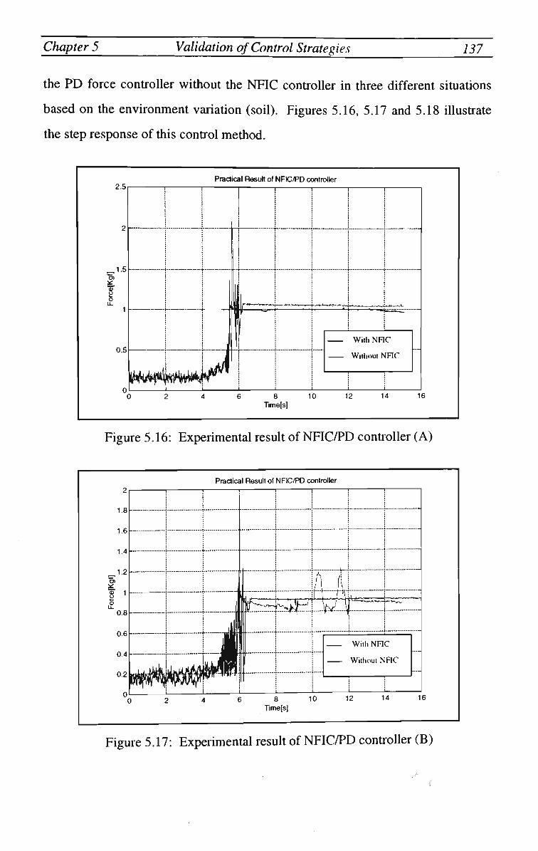
Chapter 5 Validation of Control Strategies 137
the P D force controller without the N F I C controller in three different situations
based on the environment variation (soil). Figures 5.16, 5.17 and 5.18 illustrate
the step response of this control method.
2.5
.1.5 O) __ a? LL
0.5
Practical Result ol NFIC/PD controller
!
|
i
\r—*~ r l
With NFIC
Without NFIC —
6 8 10 Time[s]
12 14 16
Figure 5.16: Experimental result of N F I C / P D controller (A)
2
1.8
1.6
1.4
_J2
"• 1
a o LL
0.8 0.6
0.4
0.2
0 (
Practical Result of NFIC/PD controller
1 ! !
1 Ij
ill
JJHI i. L JP
m™^
1 1/ w r.: T t" . / \ fj^-K^vJHl W \
i i
•*-**'_'_,
With NFIC
Without NFIC
T i • 1 1 i i ! 1 i ' i ) 2 4 6 8 10 12 14
Time[s]
....
1 6
Figure 5.17: Experimental result of N F I C / P D controller (B)

Chapter 5 Validation of Control Strategies 138
Practical Result of NFIC/PD controller
1 !
liL-ii Brr*
jl_..__uJ_,
lP "I™ IT T
nl
ip
l«J L
T
0^J u F f
- • * •
!
1
IKAw-•• .••* w—~™
v:^:;::,r r -----1
i
With NFIC
WitlioutNFIC
i j
0 2 4 6 8 10 12 14 16 Time[s]
Figure 5.18: Experimental result of NFIC/PD controller (C )
Since there is no integral term in the controller, the response has a steady state
error. Similar to the simulation results, the overshoot of the NFIC/PD method is
fairly low (5-20%) compared to the overshoot of the conventional P D force
controller which varies between 70-120%. Another problem associated with the
conventional P D force controller, which was not shown in the simulation results,
is the high oscillation of the response which results in a longer settling time.
5.4.3.2. Results of the NFIC/PDPI with Velocity Controller
In this controller (Figure 4.37), the force P D controller is implemented in
conjunction with the previous PI velocity controller. W h e n there is no
considerable impact with a stiff environment, the conventional P D force
controller (outer loop) and PI velocity controller (inner loop) are the main
controllers of the system. However, after impact detection, the NFIC impact
controller is activated to minimise the impact force. The results of the
NFIC/PIPD impact control method are compared with a PIPD controller for three
different situations in Figures 5.19, 5.20 and 5.21. It is clear from these results,

Chapter 5 Validation of Control Strategies 139
that the NFIC impact controller improves the performance of the PIPD controller
when an impact is detected. The overshoot of the NFIC/PDPI controller has
proved to be one-third of the conventional PDPI controller. It is also clear that
the settling time for the NFIC/PDPI is shorter while the PDPI method presents
more oscillatory response and accordingly, a longer settling time.
1.2
B°-8 __
o u.0.6
0.4
0.2
Practical Result ol NFIC/PDPI controller
Wt
1 1 BilLl JiJhlitLiU
1 1 i
J
_ #
IP
- "I ~ - T" • 1
t. ! J _
\ ' 1 1
. M ^-^vvw-^wlV^|f
i
With NFIC
Without N F I C
i i . . .-8
Timefs] 10 12 14 16
Figure 5.19: Experimental result of NFIC/PDPI controller (A)

Chapter 5 Validation of Control Strategies
Practical Result ol NFIC/PDPI controller
1.2
.U^M»**»
With NFIC
Without NFIC
14 16
Figure 5.20: Experimental result of NFIC/PDPI controller (B)
Practical Result of N F I C / P D P I controller 1.2
)f1«t 'itMJ><il 'i 'I "< |U*'VI»I.'«I '.'-
With NFIC
Without NFIC
12 14
Figure 5.21: Experimental result of NFIC/PDPI controller (C)
140
5.5. S u m m a r y of Results
In order to provide an overview of the performance of the intelligent controllers
produced in the experimental work, the results, in conjunction with the PI
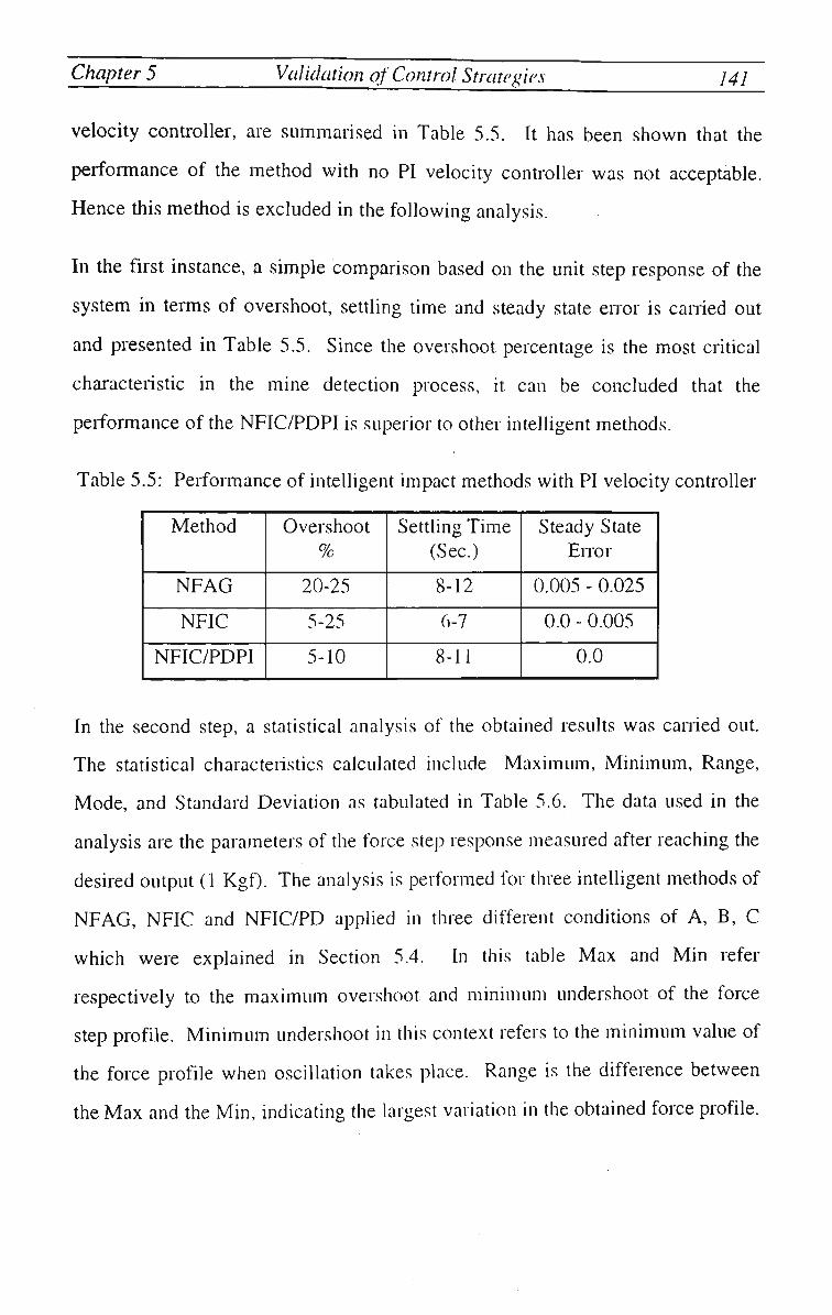
Chapter 5 Validation of Control. Strategies 141
velocity controller, are summarised in Table 5.5. It has been shown that the
performance of the method with no PI velocity controller was not acceptable.
Hence this method is excluded in the following analysis.
In the first instance, a simple comparison based on the unit step response of the
system in terms of overshoot, settling time and steady state enor is carried out
and presented in Table 5.5. Since the overshoot percentage is the most critical
characteristic in the mine detection process, it can be concluded that the
performance of the NFIC/PDPI is superior to other intelligent methods.
Table 5.5: Performance of intelligent impact methods with PI velocity controller
Method
NFAG
NFIC
NFIC/PDPI
Overshoot %
20-25
5-25
5-10
Settling Time (Sec.)
8-12
6-7
8-11
Steady State Error
0.005 - 0.025
0.0 - 0.005
0.0
In the second step, a statistical analysis of the obtained results was carried out.
The statistical characteristics calculated include Maximum, Minimum, Range,
Mode, and Standard Deviation as tabulated in Table 5.6. The data used in the
analysis are the parameters of the force step response measured after reaching the
desired output (1 Kgf). The analysis is performed for three intelligent methods of
N F A G , NFIC and NFIC/PD applied in three different conditions of A, B, C
which were explained in Section 5.4. In this table M a x and Min refer
respectively to the maximum overshoot and minimum undershoot of the force
step profile. Minimum undershoot in this context refers to the minimum value of
the force profile when oscillation takes place. Range is the difference between
the M a x and the Min, indicating the largest variation in the obtained force profile.

Chapter 5 Validation of Control Strategies 142
The smaller the Range, the better is the performance of the impact controller as it
guarantees a safer prodding.
Table 5.6: Statistical Comparison of the Intelligent Impact Control Methods
Max
Min
Range
Mode
STDEV
NFAG
A 1.04
0.935
0.105
0.975
0.0125
B 1.18
0.88
0.3
1.005
0.0418
C 1.155
0.99
0.165
1.015
0.0227
NFIC
A 1.18
0.89
0.29
1
0.0250
B 1.43
0.285
1.145
1.005
0.0421
c 1.14
0.915
0.225
1
0.0168
NFIC/PD
A 1.105
0.95
0.155
1
0.0227
B 1.09
0.95
0.14
1
0.0207
c 1.075
0.97
0.105
1
0.0094
The performance of three intelligent impact control methods are compared with
the conventional methods in Figures 5.22-5.27. These figures clearly illustrate
the superiority of the intelligent control methods over the conventional methods.
The maximum overshoots of the conventional and intelligent conhol methods are
compared in Figure 5.22. It is obvious that the NFIC/PIPD method has produced
the smallest overshoot. Another important conclusion is that the overshoots for
three different conditions A, B, and C are the same for the NFIC/PD control
method. While, for PDPI, there was about a 2 0 % variance in the overshoots of
the three conditions (Figure 5.23). This proves the robustness of the NFIC/PD
control to variation in the parameters of the environment.

Chapter 5 Validation qf Control Strategies 143
Maximum Oveshoot
35!
arvfaxjrt
mWBK Corw
Figure 5.22: M a x i m u m overshoots of the force step response
Comparison between NFIC/PDPI and PDPI
0)
> O
1.4
1.2
1
0.8
0.6
0.4
0.2
0
• Maxjnt
__ Max_Conv
NFIOPD_A NFlC/PD_B NFlC/PD_C
Figure 5.23: Focus of the previous figure on NFIC/PDPI results
Another important issue which could be crucial in mine detection task is the
extent of variation of the force profile. The smaller the variation, the more
reliable will be the prodding process. Generally, after the impact of the bayonet
with a stiff object, some unwanted oscillations take place on the force profile. A n
effective impact controller, however, can cancel or reduce the oscillations to a
satisfactory level. Figure 5.24 shows a considerable difference between the
force profile of the intelligent and conventional impact controllers. It is obvious
again that the force profile of NFIC/PD has experienced less variation than the

Chapter 5 Validation of Control Strategies 144
others and hence this method is more satisfactory. Figure 5.25 shows the same
comparison only for the intelligent impact conhol methods.
Force R a n g e
Q Rangejnl
_1 Range_Corw
Figure 5.24: Comparison of the force range of different conventional and
intelligent methods
1.2
1
0.8
0.6
0.4
0.2
M. m
i
< U-
z z
CD <
Force Range
<
< i
o Lt z
CO I
o U-
z
° 9 Lt Br z g
o CL
g u.
£L D Q-O LS. Z
p Range_lnt
Figure 5.25: Comparison of the force range of different intelligent methods
This comparison proves that variation in the range of the force amplitude for the
three conditions A, B, and C using NFIC/PD method is less than 20%.
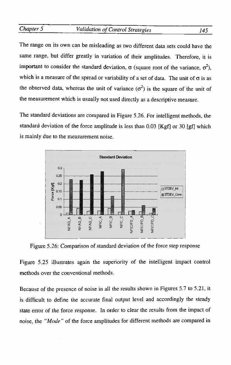
Chapter 5 Validation qf Control Strategies 145
The range on its own can be misleading as two different data sets could have the
same range, but differ greatly in variation of their amplitudes. Therefore, it is
important to consider the standard deviation, a (square root of the variance, a2),
which is a measure of the spread or variability of a set of data. The unit of a is as
the observed data, whereas the unit of variance (a2) is the square of the unit of
the measurement which is usually not used directly as a descriptive measure.
The standard deviations are compared in Figure 5.26. For intelligent methods, the
standard deviation of the force amplitude is less than 0.03 [Kgf] or 30 [gf] which
is mainly due to the measurement noise.
Standard Deviation
rjSTDEVJnt
0STDEV Corv
Figure 5.26: Comparison of standard deviation of the force step response
Figure 5.25 illustrates again the superiority of the intelligent impact control
methods over the conventional methods.
Because of the presence of noise in all the results shown in Figures 5.7 to 5.21, it
is difficult to define the accurate final output level and accordingly the steady
state error of the force response. In order to clear the results from the impact of
noise, the "Mode" of the force amplitudes for different methods are compared in

Chapter 5 Validation of Control. Strategies 146
Figure 5.27. The "Mode" of a data set provides the most commonly occurring
value when the data is restricted to specific values.
Mode
Drvbdejnt
O Mxle_Corv
Figure 5.27: M o d e values for conventional and intelligent control methods
According to this figure which illustrates the most commonly occurred value of
the force step response for conventional and intelligent methods it is feasible to
assume that these values are the final values for the force step response.
Therefore, based on these values the steady state enor of each control method
could be determined.
5.6. Conclusion
In this chapter the experimental rig used in the work has been described. The
problems encountered in commissioning the hardware and software of the rig
were also explained.
All the intelligent impact conhol methods presented in Chapter 4 were
implemented on the experimental rig and their performance were compared
against conventional control methods. It was clearly shown that the intelligent
methods produced better results.

Chapter 5 Validation qf Control Strategies 147
The NFIC/PDPI impact control method has the best performance compared to the
other two intelligent methods in terms of the range of the force variation and
percentage overshoot. These are critical parameters in the mine detection process.
The intelligent control methods have also produced better robustness and stability
to variation in the environment.
Chapter 6
MINE DETECTION
ALGORITHM

Chapter 6 Mine Detection Algorithm 149
6.1. Introduction
In the previous chapters a single-probe mechanical aim was studied for detection
of a buried object beneath the surface of the ground. During demining, after the
first encounter with an object, further prodding is needed to ensure that the
detected object is an A P mine.
In this chapter the development of a mine recognition algorithm based on
multiple prodding is described. The algorithm requires three points of a detected
object in order to estimate its features and to determine whether it is a mine. The
proposed algorithm is validated through computer simulation and experimental
work.
In addition, the design of a multi-probe mine detection mechanism is proposed in
this chapter. Such a device will detect a mine faster than a single-probe
mechanism.
6.2. Land Mine Recognition Methods
As mentioned in Chapter 2, hand prodding is the most reliable method of mine
detection and clearing. A probe is manually inserted into the soil at a 30 degree
angle, approximately every five centimetres. When a stiff object is detected,
more probing is conducted to identify the shape and size of the object. If the
object is determined to be a potential mine, a mine clearing team is called to
uncover or detonate the object.
Using this method one square metre of land is cleared in approximately four
minutes. This process of land mine detection is automated in this work. The
focus of the research is only on plastic A P mines, which are mostly cylindrical.

Chapter 6 Mine Detection Algorithm 150
Figure 6.1: A buried anti-personnel mine beneath the soil
At least three known points on a cylindrical object are needed to estimate its
geometrical properties. Hence, three consecutive probe insertions are carried out
for each iteration of the mine detection algorithm.
The distance between consecutive probing, "W", is determined based on the type
of A P mines used in the field to ensure that no land mine is missed in between the
probes. The diameter of a plastic A P mine is in the range of 5 to 10 cm (D =
5-10 [cm]) [Min96]. Hence the value of W should be chosen to be
W < D12 [cm] to ensure that the three contact points are located on the body of
the mine. This distance should not be more than 2 cm ( W = 2 [cm]) for the
smallest mine.
A n alternative approach to multiple probing is to use a multi-probe device. Figure
6.2 illustrates a three-probe mechanism in contact with an A P mine. This
diagram also illustrates the ideal configuration of the three consecutive insertions.
Another advantage of a multi-probe robot for A P mine detection compared to a
single-probe is the ability to detect whether the detected object is electrically
conductive. In a plastic mine, the resistance measured between two probes will be
quite large. Wet soil, on the other hand, has a resistance lower than a plastic
mine, but higher than a conductive object.

Chapter 6 Mine Detection Algorithm 151
c
p, 1
Robot Arm
I 4 W [_
_ """""" F
Mine
D
p
•
"S
J
Figure 6.2: The three-probe robot in contact with a mine
Generally, it is possible to identify the shape of an object by moving the probe
along the contour of the object. This, however, is not possible for an object
buried under soil.
Another constraint in the mine recognition process is that the gripper attached to
the robot end-effector cannot be a jaw type gripper to grasp the mine from two
opposite sides.
6.3. Object Recognition Procedure
The task of mine detection consists of two phases. In the first phase, three
contact points are established on the mine either through consecutive probing or
using a multi-probe device. In the second phase, the geometrical features of the
object are derived using the information provided by the three contact points.
The problem associated with the first phase is force/impact control of the arm
which was addressed in the previous chapters. In the feature extraction process,
the most important geometrical parameters of an object to be measured are the

Chapter 6 Mine Detection Algorithm 152
radius of the base and centre point location. With this information, it is possible
to determine whether or not the unknown object is of cylindrical shape.
An analytical approach to calculate the radius and centre point of an unknown
curvature based on three contact points on the boundaries is presented in Section
6.4. But, initially, a clear generic definition of an unknown 3-D object is given.
A 3 D object is defined as a combination of well-defined natural quadric surfaces
in the object reference frame, satisfying the properties of regular sets (r-sets)
[Req82] [Hah94].
6.3.1. Feature Extraction of an Unknown Object
Assuming that all three probes are in contact with the outer surface of an object,
there could be three possibilities of contact:
• Contact points are located in a planar surface which means they are in a
straight line
• Contact points are located in a concave curved surface
• Contact points are located in a convex curved surface.
For the last two cases the surface could be sphere, cylinder, cone or other
irregular curved surfaces. Since the plastic A P mine surfaces are just limited to a
cylindrical surface, a cylinder which can be represented by the lengths of the long
axis, radius and centre axis point of the base circle are the targets of this work.
Therefore, the main criteria for differentiating among different objects is the
radius and centre point location of the cylinder base circle. These values could be
used to distinguish among concave, convex, or plane surfaces. For a plane
surface the radius would be infinity while for a curved surface (concave/convex)
it is not. To distinguish between a concave from convex curved surface, the
following conditions could be examined:

Chapter 6 Mine Detection Algorithm 153
P + p if —-z-^ > P2 then it is a Concave curvature
p + P if * 3 < P2 then it is a Convex curvature
in which Px, P2 and P3 represent the probes contact points.
Alternatively, if the estimated centre point of an unknown curvature is behind the
contact points, the curvature surface is a concave curvature, which cannot be an
A P mine.
Therefore, the centre point location defines the type of the curved surface
(concave or convex) and the radius value defines whether the object is in the
range of available A P mines (2-5 [cm]). The following table categorises the type
of surfaces according to the criteria.
Condition
Oxv < P XV
Surface TyPe
Plane. Concave
O w > P XV Convex
Table 6.1: Mine possibility table
Condition
0 < R < oo Cm 5 < R < 2 Cm 2 < R < 5 Cm
Mine Possibility
No
No
No
Yes
Object Material
-
-
Conductive
Non-conductive
Mine Possibility \
No
No !
; No
No !
><J 6.4. Estimation of the Object Radius and Centre Point
In the A P mine recognition algorithm, it is essential to estimate the curvature
radius of the object in contact with the probes and decide whether it is concave or
convex. Using the information provided by the three contact points, the following
procedure is used to estimate the radius of the circular cross section of a cylinder,
as shown in Figure 6.3. It can be easily seen that

Chapter 6 Mine Detection Algorithm 154
(6.1)
where in triangle P^Py the angle 3 is
2 . "> ~> 1 1 , 1 '
A _i b +c -a
and fl = Vw2+4 b = ^W2+d;, c = V4W2-r-4
where W is the distance between the insertion points in the consecutive insertion
of the probes or the distance between probes in a multi-probe arm. The
parameters d12 , dt3 ,and d2.< are the distances between contact points:
d12=P,-P2, </13 = />-/>, </_., = /_-/>,
The following Equations (6.2) and (6.3) could be used to locate the centre of the
circle iOx , Oy) by a vector R = iR,d)with the amplitude of R and the angle
d = 0 - 90° relative to the first probe contact:
X0 = Rcosd + X p (6.2)
Y0 = R sin d + YP (6.3)
where
0=4+1+5
? _,.<r+<-2-/V 1 = cos (- 2«c
4 = tan -i W (Li 12
) 5 = cos '(-2Rc
) = cos_ 1(—) 2R

Chapter 6 Mine Detection Algorithm 155
Backward-Fo •ward Move (BF)
Left-Right Move (LR)
Probe X
Figure 6.3: Top view of the robot probes in contact with the cross section of a
cylindrical object
It is assumed so far that the mine is buried perpendicular to the ground. It is also
possible to investigate whether the cylindrical object is perpendicular to the
ground level which is important to know in mine removal. In order to find the
angle of the cylinder axis (3 in Figure 6.4), w e should have at least two vertical
contact locations on the surface of the mine. After locating a set of horizontal
contact points by three probes, the robot arm should move backward/forward
(BF) before inserting the probes into the ground to obtain another set of contact
points. It is sufficient to obtain only two contact points for each probe. Figure
6.4 shows the two contact points for one of the probes on the surface of the mine.

Chapter 6 Mine Detection Algorithm 156
Ground Level
Figure 6.4: Side view of two contact points with a mine
The angle of the cylinder axis (3) using law of Sines in the hLd12 triangle is
estimated as follows:
d\2 sin(l) sin(90"-3) sin(3 + 2)
since (1) = 30 then
h = lA dn
cos(3) (6.4)
Using the law of Cosines gives:
Is +h2 -dn cos(90° - 3) =
2hL (6.5)
Substituting (6.4) into (6.5) and simplifying the result will produce:
Asin2(jc) + flsinU) + c = 0 (6.6)
where
A = AL 4L4+4<2-8L
24
dn B = -
KL3-4L(/2
c/f2

Chapter 6 Mine Detection Algorithm 157
C = 4L2 - 3d22 and x = 2(3) or
5 x
3 = - (6.7)
It is clear from Equation (6.6), that the angle of the cylinder axis can be
calculated in terms of the difference between the penetration length of the probes
idj2) in two locations and the distance (L) between the two insertion locations.
6.5. Mine Recognition Algorithm
In this section a mine recognition algorithm is presented using the obtained
contact points and the analytical method presented in the previous section. This
algorithm which is not a finalised algorithm for mine detection is illustrated in
Figure 6.5 in the form of a flow chart. In this algorithm, which is based on three
contact points with any unknown object beneath the soil, it is vital to wait until
the insertion process of the probes is completed. The radius and centre point of
the circular intersection of a detected object is calculated according to (6.1), (6.2)
and (6.3). If three contact points can not be detected even by inserting the
maximum length of the probe, the arm should be moved to left or right. For
simplicity, it is assumed that mines are cylindrical and laid perpendicular to the
ground. The first important comparison is to check whether the calculated radius
is bigger than the maximum radius for the A P mines [Min96] which is 5 [cm].
W h e n all the three contact points are on a planar surface, the radius should be
theoretically infinity or a very large value. If the calculated radius matches that
of an A P mine (2-5 [cm]), the next step is to find out the convexity or concavity
of the curvature surface.
For a concave curvature, the centre point will locate behind all the three contact
points. It implies that Ya (the distance of the centre point from the X_axis) of the
Chapter 6 Mine Detection Algorithm 15$
center point will be negative relative to the initial location of the first probe. O n
the other hand, if the curvature surface is convex and the radius is significantly
larger than 5 [cm] or smaller than 2 [cm], the object is cylindrical but it is not an
A P mine.
Otherwise, more investigation will be necessary to decide whether the detected
object is possibly an A P mine or not. In this situation, the robot arm is moved to
left or right before the probes are inserted to obtain another set of contact points.
The above mentioned procedure will be then repeated. If the new contact points
will also produce a valid radius for a potential A P mine, the next step is to check
how similar is the new estimated radius and centre point to the previous ones.
If the estimated values in the two occasions are identical, the detected object is a
mine. Using a multi-probe arm may help at this point to determine whether the
detected object is electrically conductive.

Chapter 6 Mine Detection Algorithm 159
(v Start )
<*)
Insert Probs 4
No
Move Robot Forward
\ No y YPS
3Contacts?V5-.; Maximum? —L5=-
Register a Planar Surface
YesT
| Yes T
Calculate trie
Radius & Centre
1 T N R»?
V^T
U —
1 1 T
Move Probes Forward —•, Insert Probes
1
\ No \ R » ? y
No |
— » - 3 Contacts?
Y Calculate the | Radius & Centre
. Yes
/
S x Yes Oy<PiP2IP,? — •
Register a I Concave Surfacef
j Move Robot "^1 Forward -•(A)
No
T < R < t, •> N ° J Register a big I Convex Surface
Move Robot •i Forward — • . A :
Yes
Register a Possible Cilyndrical
Object
Move Probes Lett/Right
No (R&C).- = (R&C)?
Yes
Note: At this point several
methods could be
carried out, such as
Statistc method and
F D M S method
Register a Possible Mine
Move Robots Forward
Figure 6.5: A P mine recognition algorithm flow chart

Chapter 6 Mine Detection Algorithm 160
It is suggested to obtain two more sets of three contact points and estimate their
corresponding radii and centre points to determine the probability of having a
mine through statistical methods. Alternatively, using the fuzzy decision making
approach, it is also possible to derive the degree of certainty for the object to be a
mine. Both of these methods will be discussed in the following sections.
For simplicity, the possibility of encountering a non-vertical cylindrical object is
not considered in this algorithm. But a non-vertical cylindrical object can be
recognised at the end of the algorithm after registering a possible A P mine. This
helps to establish the angle of the cylinder axis (Equation (6.7)) which is
important for the stage of mine clearance or removal. As mentioned before,
probes are inserted at a 30 degree angle to the ground to induce half of the axial
force to the mine in contact with the probes. But if the mine is laid down with a
60 degree angle to the ground and probes are touching the top surface of the
mine, the total amount of axial force would be induced to the mine.
6.6. Simulation
A numerical simulation is carried out to illustrate how an A P mine can be
detected according to the developed algorithm. The contact points of the probe
with a circular object and four non-circular objects are used in the method. The
scenario is illustrated in Figure 6.6. The contact points of three probes for five
sets of insertions with all the objects are shown. The contact points with the
cylindrical object are located on the circle and the points for one insertion are
labelled by />, P2, and P3. For non-circular objects, the first two contact points
are the same as for the circular object ( P{ and P21 while the third contact Points
have an offset of (-1, +1, -2, +2) from /> (Figure 6.6). In this simulation the
radius and centre point of a cylindrical object with radius R = 4 [cm], located at
(X = 4 and Y = 10) is estimated for seven different insertions at a distance of 2

Chapter 6 Mine Detection Algorithm 161
[mm] from each other. Results for the circular and non-circular objects are
shown in Figures 6.7 and 6.8 by 'o', '*' and V respectively. The estimated
radii and centre points for the circular object are fairly constant in different
insertions.
Probes Movement
1....7
1. . . .7
X
Figure 6.6: Simulation based on different insertion points and different location
for the third contact points

Chapter 6 Mine Detection A Igorithm
(Cm) 10|-
Y
;> a X 8
(Cm) 4.5
4
3.5
3
2.5
2
1.5
1
0.5
0
* o <?••
~ T~ Position ol the located object
_.T. *..
* * * _ * : ^ « + :+ + : +
-I 1 1 L.
•or-rj-
* ; +1 +"••;•_••
0.5 1 1.5 2 2.5 3 3.5 4 4.5 X-axis (Cm)
Radius ol the located object
:0 0
!+ +2
3 4 Iteration
162
Figure 6.7: Simulation of A P mine recognition by multi-probe robot
Such results, however vary significantly for the third contact points in different
insertions. The radius varies from 2 to 50 [cm]. The varied centre points obtained
for the different insertions indicates that the object under study had no circular
curvature.

Chapter 6
(Cm)
Y
60
50
40
30
20
10
Mine Detection Algorithm
Centre Position ol the located objecl i i -j
++i+
+ *
: * :
o
* +
-1 -2
10 15 X-Axis (Cm)
20 25
163
60 (Cm)
50
40
30
20
(
0 •
f
*
> Cf
2
Radius of the located objecl
! ! '
: f •
t
; 4 •. : +
*f* 4* 4* 3 4 5
Iteration
i
*
+ 0
6
o * -t-
0
-2
c >
r
Figure 6.8: Simulation of A P mine recognition by multi-probe robot
Such analysis clearly indicates whether a detected object is cylindrical or not.
6.7. Experimental Results
In order to investigate the accuracy and validity of the mine detection/recognition
algorithm, a set of experiments were canned out. Since the implemented single-
probe arm had no horizontal movement to insert its probe at different points, the
buried mine and soil container are moved horizontally on the X-axis (Figure 6.3)

Chapter 6 Mine Detection Algorithm 164
by the steps of 2 cm (W= 2 [cm]) at a time to produce a similar effect. Eight
different sets of data are collected for different objects as shown in Figure 6.9.
The measurement for each object has been repeated three times for better results.
The first object is a cylindrical shape with a radius of 3.5 [cm]. Application of
the algorithm to this object indicates that it had a radius in the range of 3.33 to
3.39 [cm].
Figure 6.9: Objects which are used for experimental results
The second and third objects are two real A P mines (Ml4 and VS50) with the
radius of 2.78 [cm] and 3.8 [cm] which are detected as cylindrical objects with
radii in the range of 2.65-2.74 [cm] and 3.31-3.46 [cm]. Due to some corners on
the body of the VS50 mine (object 3), the estimation error of radius for this
object is high compared to others.
Three different stones with unknown shapes were also employed in the
experiment (Objects 4, 5, and 7). The size of stones were chosen to be in the
range of A P mines to test the accuracy of the detection algorithm. A rectangular
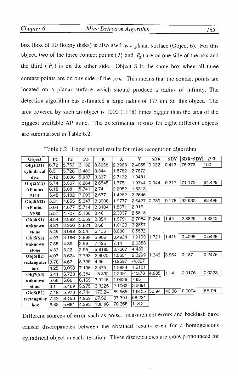
Chapter 6 Mine Detection Algorithm 165
box (box of 10 floppy disks) is also used as a planar surface (Object 6). For this
object, two of the three contact points ( P, and P2) are on one side of the box and
the third (P3) is on the other side. Object 8 is the same box when all three
contact points are on one side of the box. This means that the contact points are
located on a planar surface which should produce a radius of infinity. The
detection algorithm has estimated a large radius of 173 c m for this object. The
area covered by such an object is 1000 (1198) times bigger than the area of the
biggest available A P mine. The experimental results for eight different objects
are summarised in Table 6.2.
Table 6.2: Experimental results for mine recognition algorithm
Object
Objl(Dl)
cylindrical
disc
Obj2(Ml)
AP mine
M14
Obj3(M2)
AP mine
VS50
Obj4(Sl)
unknown
stone
Obj5(S2)
unknown
stone
Obj6(B2)
rectangular
box
Obj7(S3)
unknown
stone
Obj8(Bl)
rectangular
box
PI 6.72
6.3 7.12
5.74
6.18
5.48
5.31
5.04
5.57
3.54
3.31
5.49
4.93
7.68
4.33
4.07
3.78
4.25
5.41
5.68
6.1 7.18
7.43
6.88
P2 5.753
5.726
5.806
5.067
5.08
5.132
4.655
4.677
4.707
2.892
2.956
3.098
3.156
4.36
3.22
3.624
4.67
3.098
5.738
5.66
5.489
5.978
6.153
5.661
P3 6.132
6.483
5.987
6.264
5.741
7.003
5.347
5.714
5.138
3.569
3.821
3.04
2.898
2.99
2.95
7.793
8.735
7.196
6.384
6.169
5.975
4.744
4.969
4.393
R 3.3958
3.344
3.337
2.6545
2.74
2.677
3.3008
3.3104
3.46
3.354
3.66
3.135
3.986
7.425
5.8185
2.8075
4.96
2.475
13.832
7.9215
3.9225
173.24
67.52
138.96
X 2.3968
1.8782
2.7132
1.775
2.2052
1.4282
1.9777
1.5671
2.3037
1.9791
1.6129
3.0861
3.4934
7.14
3.7667
1.5651
0.9597
1.8994
1.2391
1.0629
2.1062
89.965
37.391
70.368
Y 2.4055
2.7672
1.9431
1.9744
1.6313
2.2646
2.6427
2.916
2.5818
2.7084
3.2857
0.5532
1.9199
2.0388
4.435
2.3299
-4.867
1.6101
-13.78
7.85
3.3091
148.05
56.221
113.2
SDK 0.032
SDY 0.413
SDR*SDY
75.373
P% 100
0.044 0.317 71.173 94.429
0.089 0.178 62.933 83.496
0.264 1.44 2.8829 3.8243
1.721 1.419 0.4095 0.5428
1.349 3.964 0.187 0.2476
4.985 11.4 0.0176 0.0228
53.94 46.36 0.0004 6E-08
Different sources of enor such as noise, measurement errors and backlash have
caused discrepancies between the obtained results even for a homogeneous
cylindrical object in each iteration. These discrepancies are more pronounced for

Chapter 6 Mine Detection Algorithm 166
non-cylindrical objects. Variation of the estimated radius for each can be
measured by the standard deviation (SD) of the calculated values. The
measurements show that the S D is quite small for a cylindrical object compared
to others. Hence the inverse of the S D is used as an index of how cylindrical is
an object. The larger the index, the higher the probability that the object is
cylindrical.
For a more reliable index, the SD of the estimated centre position is multiplied by
the standard deviation of the radius before the value is inverted to produce the
index as shown in the ten1'1 column of Table 6.2. According to the estimated
values, the index varies between 0.0004 for the worst case (the planar surface) to
75.37, for best case which is a homogeneous cylindrical disk. This range is
mapped linearly to a value between 0-100 and used as the probability that the
object can be a cylindrical object. For the A P mines the probabilities are 9 4 %
and 8 3 % while for the three stones the probabilities are 0.02%, 0.54% and 3.8%.
6.8. Fuzzy Decision Making
As an alternative approach, a fuzzy decision making algorithm has been
investigated for determining whether an object is a mine or not. This algorithm
provides the degree of certainty that an object is a mine. The fuzzy inference
systems have been successfully applied in various fields such as automatic
control, data classification, computer vision, decision analysis and expert
systems.
The basic structure of a fuzzy inference mechanism consists of three conceptual
components: a rule base, which contains a selection of fuzzy rules, a database
which defines the membership functions used in the fuzzy rules, and a reasoning
mechanism, which performs the inference procedure on the rules to produce an

Chapter 6 Mine Detection Algorithm 167
output or a conclusion. In this approach, the Mamdani Fuzzy Model [Mam75] is
employed.
A typical fuzzy rule in a Mamdani fuzzy model, consists of antecedents and
consequent:
if x is A and y is B, then z is C iw)
where A and B are fuzzy sets in the antecedent, and C is a fuzzy set in the
consequent and w is the weight of the rule which could be between 0 and 1. The
structure of a two-rule fuzzy inference system using min and max for fuzzy A N D
and O R operators and Bell-shaped membership functions is illustrated in Figure
6.10.
Inputl Input2
1(1) 1(2) max
Figure 6.10: The Mamdani Fuzzy Inference System

Chapter 6 Mine Detection A Igorithm 168
The most frequently defuzification strategy is the Centroid of Area (COA), which
is defined as:
Z-COA ~~
\z\LcU)zdz
j \ir(z)dz
where Uc(z) is the aggregated output membership function.
The developed fuzzy decision making is a Multi-Input-Single-Output (MISO)
system. The mine database [Min96] and experimental data are employed to set
up the rules and to interpret the membership functions. The input variables are
estimated Radius of an object (R), the distance of the estimated centre point from
initial position of the first probe (Y), and differences of R and Y compared to the
previous values (DR and D Y ) . The output variable is Percentage of mine
Certainty (POC). Figure 6.12 shows the schematic diagram of the fuzzy decision
making.
Radius (R)
Y.distanee (Y) _
Difference of R ( D R 1
Difference of Y (DY)_
INPUTS
FUZZY DECISIONMAKING
SYSTEM
FDMS
AF Mine Percentage of
Certainty (POC)
OUTPUT
Figure 6.11: Schematic diagram of fuzzy decision making
The range and categories of the input and output variables are described in Table
6.3. The membership functions can be tuned for a better system performance.
More experimental data and knowledge acquired from the A P mine experts may
result in a better performance by the fuzzy decision making.

Chapter 6 Mine Detection Algorithm 169
Table 6.3: Input and output variables of F D M S system and their characteristics
Input
Output
Variables Radius (R)
Y_distance (Y)
Difference of R (DR)
Difference of Y (DY)
AP Mine Certainty
Range 0-100
-100-100
0-100
0 -100
0 -100
Categories
Small Good, Big
Neg, good, VBig
Snui, Med, Big
Snui, Med, Big
Vlow, low, Medium, High, Vhigh
A trapezoidal shape is chosen to represent the membership functions of the input
and output variables as shown in Figure 6.12. The knowledge-base of the system
is a collection of intuitive rules modelling the relationship between input/output
variables. They have been developed based on the observations made in the
experimental work. The rule-base is listed in Table 6.4
Table 6.4: Rules of the fuzzy decision making
Rule 1. If (R is Small) and (Y is Neg) then (POC is Vlow) (1)
Rule 2. If (R is Small) and (Y is Too_Big) then (POC is Vlow) (1)
Rule 3. If (R is Good) and (Y is Too_Big) then (POC is low) (1)
Rule 4. If (R is Big) and (Y is Too_Big) then (POC is Vlow) (1)
Rule 5. If (R is Big) and (Y is Good) then (P(X' is low) (1)
Rule 6. If (R is Big) and (Y is Neg) then (POC is Vlow) (1)
Rule 7. If (R is Good) and (Y is Neg) then (POC is Vlow)(l)
Rule 8. If (R is Good) and (Y is Good) and (DR is Sma) and (DY is Sma) then (POC is vHigh) (1)
Rule 9. If (R is Good) and (Y is Good) and (DR is Sma) and (DY is Med) then (POC is High) (1)
Rule 10. If (R is Good) and (Y is Good) and (DR is Sma) and (DY is Big) then (POC is Medium) (1)
Rule 11. If (R is Good) and (Y is Good) and (DR is Med) and (DY is Sma) then (POC is High) (1)
Rule 12. If (R is Good) and (Y is Good) and (DR is Med) and (DY is Med) then (POC is Medium) (1)
Rule 13. If (R is Good) and (Y is Good) and (DR is Med) and (DY is Big) then (POC is low) (1)
Rule 14. If (R is Good) and (Y is Good) and (DR is Big) and (DY is Sma) then (POC is Medium) (1)
Rule 15. If (R is Good) and (Y is Good) and (DR is Big) and (DY is Med) then (POC is low) (1)
Rule 16. If (R is Good) and (Y is Good) and (DR is Big) and (DY is Big) then (POC is Vlow) (1)

Chapter 6
Mem. Degree 1
0.6
0.4
0.2
M e m Degree 1
M e m D e gf e e
Mine Detection A I go ri thin
0.5 I 15 2 5 DR
0.5 1 1.5 2 2.5 DY
Mem D.gr. i
10 20 30 40 50 60 70 P rob
Mem. D egre e 1
0 8
0 6
0 4
0.2
0
N " ' 1 T....-.,...
w
\ \
•
y •
•
,_ ,_
SO 100
Figure 6.12: Inputs and output membership functions for F D M S
170

Chapter 6 Mine Detection Algorithm 171
The experimental data presented in Table 6.2 were used to verify the fuzzy
decision making algorithm. In the algorithm, the radius, Y coordinate of the
centre point and their differences relative to another set of insertion points are
used. Hence two sets of data are obtained from three sets of insertion data for
each object. The two sets of data and relevant outputs generated by the algorithm
are tabulated in Table 6.5
Table 6.5: Input and output data for F D M S
Objects
D,
Mi
M2
Si
s2
B2
s3
B,
Iteration
1 2 1 2 1 2 1 2 1 2 1 2 1 2 1 2
Ri
3.3958
3.3958
2.6545
2.6545
3.3008
3.3008
3.354
3.354
3.986
3.986
2.8075
2.8075
13.832
13.832
173.24
173.24
Y,
2.4055
2.4055
1.9744
1.9744
2.6427
2.6427
2.7084
2.7084
1.9199
1.9199
2.3299
2.3299
-13.78
-13.78
148.05
148.05
R2
(In_D 3.344
3.337
2.74
2.677
3.3104
3.46
3.66
3.135
7.425
5.8185
4.96
2.475
7.9215
3.9225
67.5195
138.96
Y 2
(In_2)
2.7672
1.9431
1.6313
2.2646
2.916
2.5818
3.2857
0.5532
2.0388
4.435
-4.8667
1.6101
7.85
3.3091
56.2213
113.202
IR2-R1I (In_3)
0.0518
0.007
0.0855
0.063
0.0096
0.1496
0.306
0.525
3.439
1.6065
2.1525
2.485
5.91
3.999
105.72
71.4405
IY2-Y_I (In_4)
0.3617
0.4624
0.3431
0.2902
0.2733
0.0609
0.5773 2.1552
0.1189
2.5151
7.1966
0.7198
21.6263
17.0854
91.8269
34.8463
POC% (Out)
93.5945
93 93.6897
93.9231
93.9231
93.231
62.5
37.0527
25 29.7622
6.0769
25 25 6.0769 j
6.0769
6.0769
As can be seen, the Percentage of Certainty (POC) for the first three objects
which are cylindrical is about 9 3 % while for other objects P O C are mostly in the
range of 6 to 3 7 % . Considering that all the cylindrical A P mines are mostly made
of plastic material, the material of the object could also be considered as an input
variable of the F D M S . Consequently, the percentage of mine certainty (POC) of
the first object (D,) which was a metallic disc, would be very low. Figure 6.13
illustrates the output results of the F D M S system for different objects.

Chapter 6 Mine Detection Algorithm 172
AP Mine Percentage of Certainty
100
80
S* 60 -O 2 40
20
I a No, 1
| D No. 2 [
D1 M1 M2 S1 S2 B2 S3
Objects
B1
Figure 6.13: Outputs of the F D M S for eight objects
The POC for cylindrical objects (D,, M, and M2) are mostly the same for the two
sets of measurements. While the results for the other objects vary depending on
the position of three contact points on the object. The results obtained in this
method are very similar to those that were obtained in the first method.
6.9. Conclusion
In this chapter, A P mine detection/recognition methods and an algorithm based
on three contact points between the probe and the mine were studied. The three
contact points can be produced either in three consecutive insertions of the probe
or by one insertion of a multi-probe device. It was shown that the minimum gap
between three insertions or the fingers of a multi-probe device was 2 [cm] for the
A P mines used in this work.
T w o methods were presented to identify the geometrical shape of a detected
object and hence determine whether it is a mine or not. The first method was
based on the statistical characteristics of the features obtained from an object in
multiple insertion. In the second method a fuzzy decision making algorithm
estimated the percentage of certainty that a detected object was a cylindrical
mine. Both methods were validated through computer simulation and
experimental work.

Chapter 7
CONCLUSION AND FURTHER RESEARCH

Chapter 7 Conclusion and Further Research 174
7.1. Introduction
The outcomes of the work are summarised in this chapter. Although the
emphasis of this project has been on mine detection, the methodologies
developed can be applied to other applications. In this chapter, such generic
aspects of the work will be highlighted. Based on the obtained results, some
conclusions will be drawn and some directions for further work will be proposed.
7.2. Summary of the Thesis
The development of an automatic anti-personnel mine detector robot has been
reported in this thesis. The device mimics the hand-prodding de-mining
procedure by inserting a bayonet into the soil and measuring the generated force.
Detection and clearance of A P mines to a 99.6% accuracy rate is a very time
consuming and dangerous task. Therefore, the proposed robotics prodding
approach has the potential to replace the manual prodding to increase the
detection rate while preventing the accidental loss of life.
As a first step, a thorough review of the previous work in this area was carried
out. In particular, the contact and non-contact methods employed by other
research groups for detection of a mine were studied. This review confirmed that
A P mine detection is an active and promising research area, requiring a great
deal of research and development for a satisfactory outcome.
The properties of the soil and the objects encountered during prodding are
unknown prior to the operation. Hence the demining robot will be operating in
an unstructured or semi-structured environment. In addition, there is a sudden
change in the stiffness of the environment as the robot enters the soil or
encounters an object. This will create an impact on the manipulator.

Chapter 7 Conclusion and Further Research 175
Due to these varying conditions, conventional mathematical modelling and
control of the robot and its environment will not produce a satisfactory outcome.
Consequently, the overall system was modelled using a neuro-fuzzy method
called Adaptive Spline Modelling of Observation Data ( A S M O D ) . Force/impact
conhol was introduced to maintain system stability during sudden changes in the
stiffness of the environment.
A study of the impact phenomenon provided some guidelines on the design of
the robot and its control system. It was shown that the sampling time for the
digital controller should be as short as possible to minimise the effect of the
impact force. On the other hand, the sampling time should be long enough to
allow the complete execution of the control algorithm. The mass of the robot
contributes significantly to the magnitude of the impact force. Hence, it is
important to design the robot as light as possible.
A number of intelligent force/impact control algorithms were developed in the
study. The structure of all these algorithms was based on the explicit force
control, including a velocity control loop inside an external force/impact conhol
loop. The intelligent control schemes for the prodding arm were based on the
inverse dynamic model of the robot arm in contact with the environment.
Overall, two main intelligent control schemes the Neuro-Fuzzy Adaptive Gain
( N F A G ) and the Neuro-Fuzzy Impact Control (NFIC), including some sub-
driven control schemes from the NFIC, were developed and validated.
The developed models were validated through both computer simulation and
experimental work. The intelligent control algorithms outperformed the
conventional controllers in all of the case studies. They also produced
performances acceptable for demining operation.
Chapter 7 Conclusion and Further Research 176
Finally, an algorithm was developed to distinguish an A P mine from other types
of objects. The algorithm is based on three contact points obtained from an
object either through three consecutive insertions of the probe or one insertion of
a multi-probe device. The degree of certainty for a detected object to be a mine
was determined through two methods using statistical and fuzzy approaches.
The performance of the algorithm was validated through computer simulation
and experimental work.
7.3. Future Research
The work earned out in this study can be considered as the first step towards the
development of a realistic and practical automatic robotic deminer. Further work
is required in different areas to complete the work. They will include:
• Development of a multi-probe arm. This will enhance both the reliability and
speed of the demining process.
• Further work on the object recognition algorithm for a more robust and
reliable method.
• Enhancement of the neuro-fuzzy model based on the input/output data
collected from the field operation of the prototype deminer. This approach
was successfully used for the peg-in-hole insertion task [Sha97].
• Proper design and development of the mechanical and electronic hardware of
the deminer for optimum field performance.
• Design and development of a reliable computing platform suitable for the field
implementation of the control algorithm.

Chapter 7 Conclusion and Further Research 177
• Design and development of a mobile robot to navigate the deminer arm in the
field. Simplicity of the design, low cost, and low weight are important criteria
to consider. In addition, the weight distribution on the feet or wheels should
be studied to minimise the resultant force on each foot or wheel to avoid
triggering the mine. The mobile robot should also have proper drive systems
for navigation on various types of ground, including flat and bumpy areas,
covered by soft, sticky, hard soil (sand, mud, rock), and vegetation.
Alternatively, different types of driving mechanism may be designed for
different types of surfaces.

REFERENCES
[Ake94] P. Akella, V. Parra-Vega, S. Arimoto, K. Tanie, "Discontinuous Model-
based Adaptive Control for Robot Executing Free and Constrained Tasks", Proceedings of the International Conference on Robotics and Automation,
IEEE, pp. 3000-3007, USA, 1994.
[A1192] B. Allotta, G. Buttazzo, "Impact Handling by Proximity and Force Sensing", Proceedings of the IEEE International Conference on Robotics and Automation, pp. 2032-2037, CA, USA, 1992.
[And88] R. J. Anderson, M. W. Spong, "Hybrid Impedance Control of Robotic Manipulator", IEEE Journal of Robot. Automat., Vol.4, No. 5, pp.549-556,
Oct. 1988.
[Ant95] D. Antonia, I. Ralkovia, "Ground Probing Sensor for Automated Mine
Detection," K o R E M A , Opatija 1996. http://www.rasip.fer.hr/~d/mine_project.html
[Ara96] R. Araujo, U. Nunes, A. T. de Almeida, "Fuzzy-Based Reinforcement Learning of a Robot Force Control Skill", Proceedings of the IEEE International Symposium on Industrial Electronics (ISIE'96), Vol. 1, pp.
453-458,1996."
[Asa90] Haruhiko Asada, "Teaching and Learning of Compliance Using Neural Nets: Presentation and Ceneration of Nonlinear Compliance," Proceedings of the IEEE International Conference Robotic and Automation, pp. 1237-
1244, 1990.
[Ast95] K. Astrom, B. Wittenmark, "Adaptive Control", 2nd ed, Addison-Wesley.
New York, 1995.
[Aze95] S. G. Azevedo, D. T. Gavel, J. E. Mast, and J. P. Warhus, "Landmine Detection and Imaging using Micropower Impulse Radar (MIR)" Workshop on Anti-Personnel Mine Detection and Removal, pp: 48-51, Lausanne,
1995.
[Bog93] S. Bogdan, Z. Kovacic, "Fuzzy Rule-based Adaptive Force Controll of a Single D O F Mechanisms," Proceedings of the International Symposium on
Intelligent Control, pp.469-474, USA, 1993.
References 179
[Bos95] K. M. Bossley, "Neuro-fuzzy construction algorithms", Technical Report,
Dept. of Electrical and Computer Science, University of Southampton, 1995.
[Bro94] M. Brown, C. Harris, "NeuroFuzzy Adaptive Modelling and Control," Prentice Hall, U K , 1994.
[Bro98] J. W. Brooks, J. D. Nicoud, "applications of GPR Technology to
Humanitarian Demining Operations in Cambodia: Some Lessons Learned," Proceedings of the Third Annual Symposium on Technology and the Mine Problem, Mine Warfare Association, Monterey, CA, USA, 6-9.4.1998.
[Bru94] B. Brusmark, S. Abrahamson, D. Axelsson, A. Gustafsson, H. Strifors, "Evaluation of Experimental Data from a G P R System for Detection and Classification of Buried Mines", Proceeding GPR'99, Kitchener, pp639-643, June 1994.
[Bru96] C. Brushini, et. al. "Groun Penetrating RADAR Induction Coil Sensor Imaging for Antipersonnel Mines Detection", 6th International Conference on Ground Penetrating RADAR (GPR'96), Sendai, Japan, 30 Sep.-3 Oct. 1996.
[Bru97] C. Bruchini, and B. Gros, "A Survey of Current Sensor Technology Research for the Detection of Landmines", Proceeding of the International Workshop on Sustainable Humanitarian Demining (SusDem'97), Zagreb, Croatia, 29 September-1 October 1997.
[Car94] M. Carlin and et. al. "A comparison of four methods for nonlinear data modelling," Chemometrics and Intelligent Laboratory Systems, Vol. 23, PP,
163-178, 1994.
[Car95] J. de Carufel, D. S. Necsulescu, "Model Predictive Control for Impact-Contact Motion of a Manipulator" Proceedings of Canadian Conference on
Electrical and Computer Engineering , pp. 330-333, IEEE, NY, USA,
1995.
[Chi95] R.J. Chignell, "Ground Probing Radar- A Technology Ready for Mine Detection Equipment Development", Proceedings of the Workshop on Anti-Personnel Mine Detection and Removal, pp52-59, 1995.
[Chi97] D. K. Chiu, S. Lee, "Design and Experimentation of a Jump Impact Controller", IEEE Control Systems Magazine, pp. 99-106, June 1997.
[Cox90] M. G. Cox, "Algorithms for Spline Curves and Surfaces", NPL Report
DITC166, 1990.
[Cra94] R. F. Craig, "Soil Mechanics' Fifth Edition, Chapman & Hall, London, UK,
1994.

References 180
[Dan97] D. J. Daniels, "Radar Rechniques for Mine Detection", Proceedings of
International Workshop on Sustainable Humanitarian Demining, pp. S5.1-9, Zagreb, October, 1997.
[Daw97a] Kenneth M. Dawson-Howe and Tomos G. Williams, "Autonomous Probing
Robots for the Detection of Abandoned Landmines", Proceedings of the 5th Symposium on Intelligent Robotics Systems (SIRS-97), pp.51-58, Stockholm, Sweden, 8-11th July 1997
[Daw97b] Kenneth M. Dawson-Howe and Tomos G. Williams, "Automating the Probing Process", Proceeding of the International Workshop of Sustainable Humanitarian Demining, Zagreb, Croatia, 29th September-1st October 1997.
[Daw98] Kenneth M. Dawson-Howe and Tomos G. Williams, "The Detection of Buried Landmines Using Probing Robot" (to appear - probably June/July 1998).
[Fri95] M. Fritzsche, P. Trinkhaus "Detection of Buried Landmines Using Ground Penetrating Radar and a Metal Detector First Results of Field Experiments," Workshop on Anti-Personnel Mine Detection and Removal, pp: 44-45, 1995.
[Gol60] W. Goldsmith, "Impact: The Theory and Physical Behaviour of Colliding Solids", London, Edward Arnold Publishers, 1960.
[Gue97] F. Gueme, et. al., "GPR Mine Sensors for Data Acquisition in the Field", Proceedings of the International Workshop on Sustainable Humanitarian Demining (SusDem'97), Zagreb, Croatia, 29 September-1 October 1997. (See also http://diwww.eptl.ch/W31ami/detec/susdem_detec2.html).
[Hah94] H. Hahn, "Recognition of 3D Objects by a 3-fingered Robot Hand Equipped with Tactile and Force Sensors", Proceedings of the International Conference on Multi-sensor Fusion and Integration for Intelligent Systems,
IEEE, USA, 1994.
[Ham96] H. Hampric, "New Approaches to Mine Detection", Pre-conference paper at the International Conference on Mine Clearance Technology, Working Group IX, Copenhangen, Denmark, 2-4 July, 1996, (See also
http://www.demining.brtrc.com/).
[Har94] C. J. Harris, C. G. Moore, M. Brown, "Intelligent Control: Aspects of Fuzzy Logic and Neural Nets", World Scientific Series in Robotics and Automated
System, Vol. 6,'1994.
[Hog85] N. Hogan, "Impedance Control: An Approach to Manipulation," Journal of Dynamic Systems, Measurement, and Control, pp. 1-25, Vol. 107, March
1985.

References jg
[Hun92] K. J. Hunt, D. Sbarbaro, R. Zbikowski, P. J. Gawthrop, "Neural Networks
for Control Systems-A Survey", Automatica, Vol. 28, pp. 1083-1112, 1992.
[Hyd94] J, M. Hyde, M. R. Cutkosky, "Controlling Contact Transition", IEEE
Control Systems Magazine, pp. 25-30, February 1994,
[Intl] The Internet Home Page on Direct and Indirect Consequences of Land
mines on Public Health, at http://www.demining.brtc.com/content.
[Int2] The Internet Home Page of The International Committee of the Red Cross
at http://www.icrc.ch/icrcnews/3a 1 a.htm.
[Kav92] T. Kavli, "Learning Principles in Dynamic Control", Dr. Sci Thesis,
Institute for Informatics, University of Oslo, Norway, 1992.
[Kav95] T. Kavli, E. Weyer/'On ASMOD - An algorithm for empirical modelling
using spline functions", Neural Netn'orks Engineering In Dynamic control
Systems, pp83-l()4, Springer Series on Advances in Industrial Control,
1995.
[Kaz88] K. H. Kazeroni, B. J. Waibel, "Theory and Experiment on the Stability of
Robot Compliance Control", Proceedings of the IEEE International
Conference on Robotics and Automation, pp. 7 1-87, 1988.
[Kig951 K. Kiguchi, T. Fukuda, "Fuzzy Neural Controller for Robot Manipulator
Force Control," Proceedings of forth IEEE International Conference on
Fuzzy Systemsy'ol. 2, pp. 869-874, 1995.
[Kim95] S. W. Kim, H. S. Non, D. M. Woo, M. Park, "Hybrid Force/Position Robot
Control Using An Adaptive Fuzzy Control Method", Proceedings of
International IEEE/RSJ on Intelligent Robots and Systems, Vol. 1, pp. 316-
321,1995.
[Kos92] Bart Kosko, "Neural Networks and Fuzzy Systems" Prentice Hall, USA,
1992.
[Lee96] E. Lee, "A Nonlinear Bang-Bang Impact Force Control", IEEE Proceedings
of the 35th Conference on Decision and Control, pp. 1967-1973, NY, USA,
1996.
[Mam75] E. H. Mamdani, S. Assilian, "An Experiment in Linguistic Synthesis with a
Fuzzy Logic Controoler", International Journal of Man-machine Studies,
pp. 1-13, 1975.
[Man93] N. Mandal, S. Payandeh, "Experimental Evaluation of the Importance of
Compliance for Robotic Impact Control", Second IEEE Conference on
Control Applications, Vancouver, B.C., pp. 511-516, September 1993.

References 182
[Mai-94] G. T. Marth, T. J. Tarn, A. K. Bejczy, "An Event Based Approach to
Impact Control: Theory and Experiments", Proceedings of the IEEE
International Conference on Robotics and Automation, pp. 918-923, CA USA, 1994.
[Mas96] M. Shibatam T. Murakami, " A Unified Approach to Position and Force
Control by Fuzzy Logic," IEEE Transactions on Industrial Electronics, Vol. 43, No. 1, pp. 81-87, 1996.
[Mat96a] MATLAB Compiler User's Guide, October 1996.
[Mat96b] MATCOM V2.0 C++ Compiler User's Guide, August 1996.
[Mil90] W. Miller, R. Sutton, P. Werbose, "Neural Networks for Control," MIT Press, USA, 1990.
[Min96] MineFacts Data base, Department of Defence, United States of America, 1996.
[Moo93] K. L. Moore, "Iterative Learning Control for Deterministic Systems," Springer-verlag, Germany, 1993.
[Mor96] K. A. Morgansen, F. G. Pin, "Impact Mitigation Using Kinematic Constraints and the Full Space Parameterisation Method", Proceedings of the IEEE International Conference on Robotics and Automation, pp. 1897-
1902, 1996.
[Nel95] B. J. Nelson, J. Danniel Morrow, P. K. Khosla, "Fast Stable Contact Transition with a Stiff Manipulator Using Force and Vision Feedback", IEEE/RSJ International Conference on Intelligent Robots and Systems,
IEEE Computer Society Press, pp. 90-95, 1995.
[Nic95] J. D. Nicoud, Ph. Machler, "Pemex-B a Low Cost Robot for Searching Anti-Personnel Mines, " Workshop on Anti-Personnel Mine Detection and
Removal, pp: 26-29, Lausanne, 1995.
[Nic96] J. Nicoud, "Mine Clearance: not only a problem for the military any more", 6th International Symposium on Measurement and Control in Robotics
(ISMCR'96), Brussels, pp. 6-10, May 1996.
[Oga97] K. Ogata, "Modern Control Engineering ", 3nl Edition Prentice Hall, USA,
1997.
[Oh94] Y. H. Oh, W. K. Chung, K. W. Jeong, Y. Youm, "Implementation of Passive Hardware Damper for Force and Impact Control", Proceedings of the IEEE International Conference on Robotics and Automation, pp. 937-
943, CA, USA, 1994.

References 183
[Oma96] S. Omatu, M. Khalid, "Neuro-Control and its Applications: Advances in
Industrial Control", Springer, UK, 1996.
[Rai811 M. H. Raibert, J. J. Craig, "Hybrid Position/Force Control of Manipulators",
ASME Journal of Dynamic Systems, Measurments and Control, Vol. 102,
pp. 126-133, 1981.
[Req82] A. G. Requicha, H. B. Voelcker, "Solid Modelling: A Historical Summary
and Contemporary Assessment", IEEE CG&A, pp. 9-24, 1982
[Ros61] F. Rosenblatt, "Principles of Neurodyn amies: Perceptrons and the Theory
of Brain Mechanisms", Spartan Books, Washington DC, 1961.
[Sal80] J. K. Salisbury, "Active Stiffness Control of a Manipulator in Cartesian
Coordinates," Proceeding of 19th IEEE Conf On Decision Control, pp. 95-
100, Dec. 1980.
[Sha97] A. M. Shahri, F. Naghdy, P. Nguyen "Neuro-Fuzzy Compliance Control
with the Ability of Skill Acquisition from Human Experts", Proceedings of
the International Conference and Workshops on Conventional and
Knowledge-Based Engineering Systems (KES'97), pp. 442-448, Vol 2,
Adelaide, Australia, May 1997.
[Shi96] M. Shibatam, T. Murakami, " A Unified Approach to Position and Force
Control by Fuzzy Logic," IEEE Transactions on Industrial Electronics,
Vol. 43, No. 1, pp. 81-87, 1996.
[Sil95] C. W. de Silva, "Intelligent Control: Fuzzy Logic Applications;1 CRC Press,
USA, 1995.
[Ska96] D. Skaley, J. Hemsing, and K.R. Fyfe, "A Mechanical Means of Land Mine
Detection", Project Report for DRES DND, Canada, 1996.
http://www.mece.ualberta.ca/landmine.html
[Sta94] Statement of the United Nations Secretary-General, Assistance in Mine
Clearance, 49,h Session, Item 22 of the Agenda A/49/357, p2, 6 September
1994.
[Suh94] I.H. Suh, K.S. Eom, and H.J. Yeo, "Explicit Fuzzy Force Control of
Industrial Manipulators with Position Servo Drivers," IEEE/RSJ/GI
International Conference on Intelligent Robot and. Systems, pp. 657-664,
Vol. 1, USA, 1994.
[Suk96] S. Lee, D. Chiu, "Performance Robustness of Manipulator Collision
Controller", Proceedings of IEEE/RSJ International Conference on
Intelligent Robots and Systems, USA, 1996.
[Taf95] S. Tafazoli, C. W. de Silva, P. D. Lawrence, "Position and Force Control of
an Electrohydrulic Manipulator in the Presence of Friction", IEEE

References 184
International Conference on Systems, Man and Cybernetics, pp. 1687-1692, NY, USA, 1995.
[Tai-96] T. Tarn, Y. Wu, N. Xi, A. Isidori, "Force Regulation and Contact Transition
Control", IEEE Control System Magazine, pp. 32-40, February 1996.
[Tar97] M. Tarokh, S. Bailey, "Adaptive Fuzzy Force Control of Manipulators with
Unknown Environment Parameters", Journal of Robotic Systems, Vol. 14, No. 5, pp. 341-353, 1997.
ITor96] A. Tornambe, "Modelling and Controlling One-Degree-of -Freedom
Impacts", IEE Proceedings, Control Theory Application, Vol. 143, No. 1, pp. 85-90, January 1996.
[Tou89] K. Y. Toumi, D. A. Guts, "Impact and Force Control", IEEE International
Conference on Robotics and Automation, pp. 410-416, IEEE Computer Society Press, USA, 1989.
[Tre97] J. Trevelyan, "What Can Robotics Researchers Learn form the Land Mine
Problem?", Proceedings of the International Conference on Field and
Service Robotics, pp. 516-522, Canberra, Australia, 8-10 Dec. 1997.
[Tsi96] K. Tsipis, "Report on the Landmine Brainstorming Workshop of Aug. 25-
30, Nov. 96", Report #27, Program in Science & Technology for
International Security, MIT, Cambridge, M A , USA, 1996.
http://mcnutt.mit.edu/PSTIS/minereport/minereport.html
[Vol91] R. Volpe, P. Khosla, "Experimental Verification of a Strategy for Impact
Control", Proceedings of the 1991 IEEE International Conferences on
Robotics and Automation , Sacramento, California, pp. 1854-1860, April
1991.
[Vuk94] M. Vukobratovic, and A. Tuneski, "Contact Control Concepts in
Manipulation Robotics- An Overview, " IEEE Transaction on Industrial
Electronics. Vol.41 No. 1, Feb. 1994.
[Wal94] I. D. Walker, "Impact Configurations and Measures for Kinematically
Redundant and Multiple Armed Robot Systems", IEEE Transactions on
Robotics and Automation, Vol. 10, No. 5, pp. 670-683, October 1994.
[Wan93] L. Wang, "Stable Adaptive Fuzzy Control of Nonlinear Systems", IEEE
Transactions on Fuzzy Systems, Vol. 1. No. 2, pp. 146-155, May 1993.
[Was931 P. D. Wasserman 'Advanced Methods in Neural Computing: Series in
Advances in Industrial Control, " Van Noslrand Reinhold, USA, 1993.
[Wed88] D. L. Wedel, G. N. Saridis, "An Expriement in Hybrid Position/Force
Control of a Six D O F Revolute Manipulators", Proceedings of the IEEE
International Conference of Robotics Automation, pp. 1638-1642, 1988.

References 185
[Wen96] S. Weng, K. Young, "Robot Impact Control Inspired by Human Reflex",
Proceedings of the IEEE International Conference on Robotics and
Automation, pp. 2579-2585, Minneapolis, Minnesota, April 1996
[Wey95] E. Weyer, T. Kavli, "The ASMOD algorithm: some new and theoretical and
experimental results," Internal Report, SINTEF, 1995.
[Whi85] D. E. Whitney, "Historical Perspective and State of the Art in Robotic Force
Control", Proceedings of the IEEE Conference on Robotics Automata, pp. 262-268, 1985.
[Wu95] Y. Wu, T.J. Tarn, N. Xi, "Force and Transition Control with Environmental
Uncertainties", Proceedings of the IEEE International Conference on
Robotics and Automation, pp. 899-904, 1995.
[Wu96] Y. Wu, T.J. Tarn, N. Xi, and A. Isidori," On Robust Impact Control via
Positive Acceleration Feedback for Robot Manipulators", Proceedings of
the IEEE International Conference on Robotics and Automation, pp.1891-
1896, Minneapolis, Minnesota, USA, April 1996.
[Xu88] Y. Xu, R. Paul, "On Position Compensation and Force Control Stability of a
Robot With a Compliant Wrist", Proceedings of the IEEE Conference on
Robotics and Automation, pp. 1173-1178, IEEE, 1988.
[Yon93] K. P. Yong, S. C. Hyung, "A Fuzzy Ruled-Based Assembly Algorithm for
Precision Parts Mating," Mechatronics Vol. 3, No. 4, PP. 433-450, 1993.

Appendix A:
MATCOM COMPILER
A.l. Introduction
In this part an explanation on using MATCOM compiler which enables to create
a standalone program using M A T L A B .m files will be provided. It should be
mentioned that DJGPP is selected as the C++ compiler and D O S as the platform
to run the executable files. As there are different M A T L A B functions which
should be called inside the C++ program and there are also some functions
supporting the PC30-C board, the best way of building standalone executable
application is to use a makefile which is given below.
A.2. Makefile for Building Standalone Executable Application
In the following makefile the output is co32cl.exe which can be run in DOS
environment.
#
# M A T C O M makefile for DJGPP : Target GG32
#
all: co32cl.exe mapdata.cpp: mapdata.m
d:/matcom/matcom mapdata.m mapdata.cpp -mat2cpp -nologo
mapdata.o: mapdata.cpp gcc -c -Id:/matcom/ -w -L./ -I./ -o mapdata.o mapdata.cpp
fndKVInd.cpp: fndKVInd.m d:/matcom/matcom fndKVInd.m fndKVInd.cpp -mat2cpp -nologo
fndKVInd.o: fndKVInd.cpp gcc -c -Id:/matcom/ -w -]_./ A.I -o fndKVInd.o 1'ndKVInd.cpp
computeB.cpp: computeB.m d:/matcom/matcom computeB.m computeB.cpp -mat2cpp -nologo

Appendix A 187
computeB.o: computeB.cpp
gcc -c -Id:/matcom/ -w -L./ -I./ -o computeB.o computeB.cpp cmpBasis.cpp: cmpBasis.m
d:/matcom/matcom cmpBasis.m cmpBasis.cpp -mat2cpp -nologo cmpBasis.o: cmpBasis.cpp
gcc -c -Id:/matcom/ -w -L./ -I./ -o cmpBasis.o cmpBasis.cpp cmpSplBs.cpp: cmpSplBs.m
d:/matcom/mateom cmpSplBs.m cmpSplBs.cpp -mat2cpp -nologo
cmpSplBs.o: cmpSplBs.cpp
gcc -c -Id:/matcom/ -w -L./ -I./ -o cmpSplBs.o cmpSplBs.cpp
tmult.cpp: tmult.m
d:/matcom/matcom tmult.m tmult.cpp -mat2cpp -nologo
tmult.o: tmult.cpp
gcc -c -Id:/matcom/ -w -L./ -I./ -o tmult.o tmult.cpp
djpc30s.o: djpc3()s.cpp gcc -c -Id:/matcom/ -w -L./ -I./ -o djpc30s.o djpc30s.cpp
djpc30d.o: djpc3()d.cpp gcc -c -Id:/matcom/ -w -L./ -I./ -o djpc.3()d.o djpc30d.cpp
g_co32cl.o: g_co32cl.cpp gcc -c -Id:/matcom/ -w -L./ -I./ -o g_co32cl.o g_co32cl.cpp
go32cl.exe: mapdata.o fndKVInd.o computeB.o cmpBasis.o cmpSplBs.o tmult.o djpc30s.o djpc30d.o
g_co32cl.o gcc -Ld:/matcom/ -w -L./ -I./ -o co32cl.exe («>co32cl.rsp -s -lmlihO -lmlibl -Igpp -lm -lpc
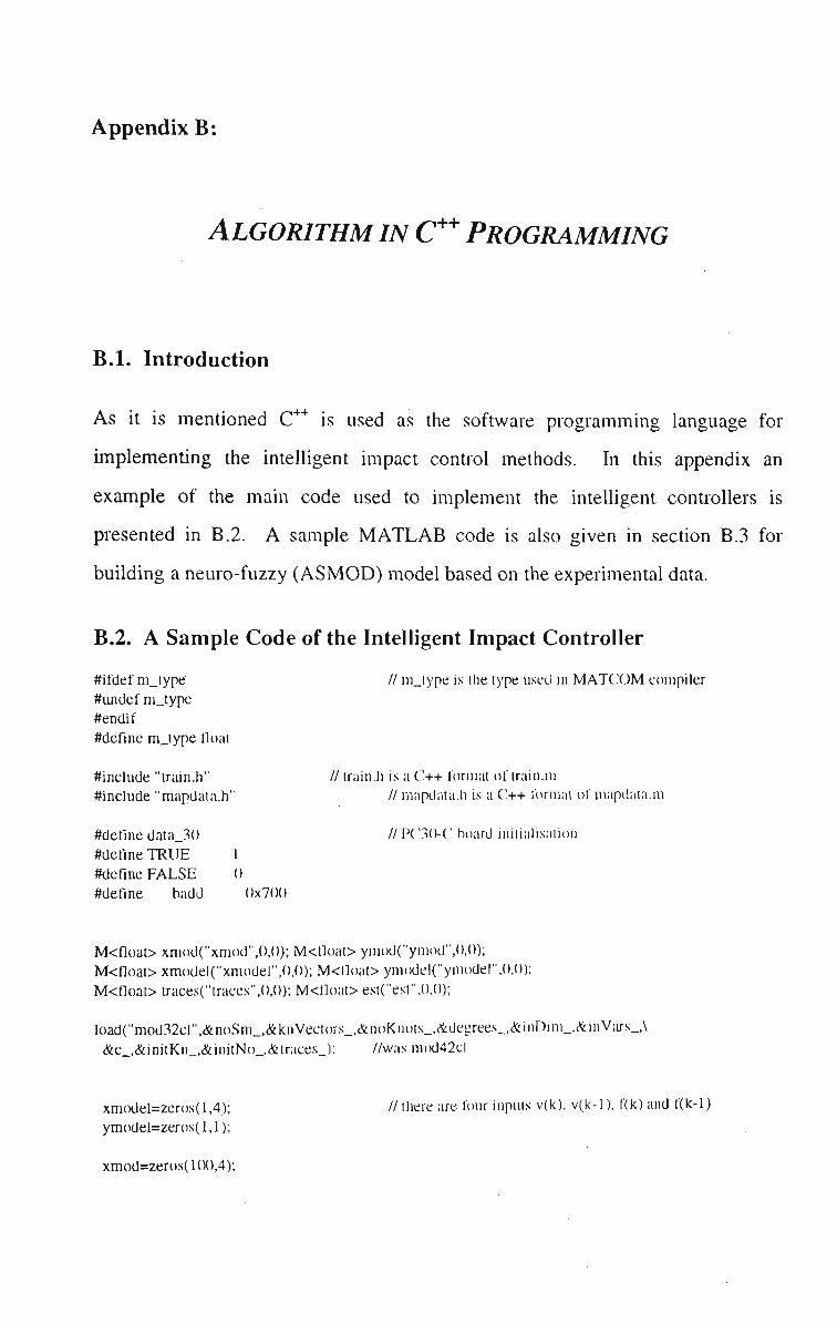
Appendix B:
ALGORITHM IN C++ PROGRAMMING
B.l. Introduction
As it is mentioned C++ is used as the software programming language for
implementing the intelligent impact control methods. In this appendix an
example of the main code used to implement the intelligent controllers is
presented in B.2. A sample MATLAB code is also given in section B.3 for
building a neuro-fuzzy (ASMOD) model based on the experimental data.
B.2. A Sample Code of the Intelligent Impact Controller
#ifdef m_type // m_type is the type used in MATCOM compiler
#undef m_type #endif #define m_type float
#include "train.h" // train.h is a C++ format of train.m #include "mapdata.h" // mapdata.h is a C + + formal of mapdata.m
#define data_30 // PC30-C board initialisation
#deflne T R U E 1 #define F A L S E 0
#define badd 0x700
M<float> xmod("xmod",0,0); M<float> ymod("ymod",0,0);
M<float> xmodel("xmodel",0,0); M<float> ymodel("ymodel",0,0):
M<float> traces("traces",0,0); M<tloat> est("est",(),0);
load(•,mod32cl^&n()Sm_,&knVcct()rs_,&nl)Kn()ts_,°rees_,&iI)Dinl_,&inV;trs_,\
&c_,&initKn_,&initNo_,&traces_): //was mod42cl
xmodel=zeros(l,4); // there are four inputs v(k), v(k-l), f(k) and f(k-l)
ymodel=zeros(l,l);
xmod=zeros(HX),4);

Appendix B
ymod=zeros(100,l);
signed int d_a[20000];
FILE *fp_in; /* pointer to a tile */
unsigned int vout, vsign=0; // zero is for forward direction float varm=0.0, varm 1=0.0;
float xl.vl, outfc;
float x.f.finit;
float df,mf,mfl,yf,temp;
float vel, freq, errorv, errorvl=0.0, errorv2=0.0. xinit;
float ke, kf, errorf,errorf_l=0, vpwm, Deltaf=0.0; //outfc=0.0.vl,xl int N=660, counter= 100;
float refrence =1.0, refrence_l=0.0, r=().()12, vl_l=0, f_l=0, x_l=0,f_2, dx; float aO=428.235, al=-237.765, a2=0.0, hl= -1.0; //digitized PI controller
float aa0=0.02, aal=-0.03, aa2=0.01, bbl= -1.0: float farm, farm 1=0.0, errorfl=0.0, errorf2=0.0;
float outtPI=0.0, outfPI_l=0.0. sampling_freq=100.0:
uclock_t end_timel, end_time2, end_time21, initjime, startjime;
float delai, loop_time, exec_time, progjime, ymodel_l=0; int dela, ind;
unsigned int omega,count;
char inf[20]; register int i,j;
float m, lim; int tl=0;
U /*** Declarations for openning the data file ********/
char f_name[40]: /* buffer for file name */
char file; clrscr(); printf("\n\r (Press E S C to exit) " ) ;
printf("\n D o you want to save data in a file '.' [y/n]:"):
file = getcharQ;
if (file =='y' II file == 'Y') { printf(" Enter file name :\t");
scanf("%s",f_name); fp_in = fopen(f_name,"w"): /* Open the tile */
if(fp_in==NULL) {
printf("\n Can not open the file" );
exit(l);
} else printf("\n FILE O P E N E D \n");
} printf("Press any key to start: \n"); getch();
base_30 = badd; if (diag()) printf("\n PC-30 fault."):
else if (type_30 < found_39) printf("\n PC-3U, PC-30B, PC-30C, PC-30D or PC-30 P G required."):
else { init(); // for 2khz sampling period which is 1msec for each sample

Appendix B 190
ad_prescaler(5); // set the prescaler of the A D C ad_clock(4); // set the clock rate of the A D C for (i = 0; i < 5; i++) set_gain(i, 0);
cntr_cfg(0); // set the counter mode
1
ad_in(5, &d_a[l]); // position sensor // initial position sensor
xinit=((-(d_a[l] - 4()95)/16.25)-6.523077-l/16.25)/1000; // 16.25 is the calibration coefficient [m] ad_in(l, &d_a[0]); // force sensor
// initial force sensor
finit=(d_a[0]-2048)*5 -40; // 5 is the calibration coefficient [grf]
f_l=finit*0.001;
// Timer Initialisation
init_time = uclockQ;
count = 30000 - cntr_read(); cntr_write(30000); // load the counter
end_time2 = uclock();
end_time21 =end_time2;
while(l){ if(kbhit()) { if (getchQ = '\xlB') /* check for E S C character */
break;
1 III****** Getting Data (begining of the main i o o p ) * * * * * * * * * * * * * * * / counter =counter +1; ad_in(l, &d_a[0]); // force sensor ad_in(5, &d_a[l]); // position sensor
f=(d_a[0]-2048)*5-finit: x=(-(d_a[l] - 40lA5)/16.25)-6.523077: // 16.25 is the calibration coefficient
count = 30000 - cntr_read(); cntr_write(30000); // initialize counter for next loop
if(count >= 200 ) count = count_l; freq=(count*sampling_freq*2.0)/N: // [Hz]. N=f>60 , *2 is for nip-Hup
if (freq > = 33) freq=32.0; // 32 is max speed at 12 volt vel=freq*0.00175: //Linear Velocity [m/sec] pitch=1.75 [mm]
i///***************+ Control Procedure *************
xl=((x/1000)-xinit): // manipulator position [m]
// FILTER T O C A N C E L F O R C E N O I S E mf=(t71(XM).())-(-().«6yy*mn); // it was (-O.o065;|:mfl):
yf=0.1331 *mfl; //it was 0.3(J35*mfl: // [kgl'J
mfl=mf; // in order to define the direction of speed we should check the
// voltage of the motor drive.
if(varm>=0) vl=vel;
else vl=-vel;
xmodel.r(l)=vl;
xmodel.r(2)=vl_l;
errorf=(refrence- (f*().(K)l))*l.():
xmodel.r(3)=errorf* 1.0;
xmodel.r(4)=errorf_l * 1.0:
// without force filter // this is to be used in model as controller
ymodel=mapdat a( xmode 1):
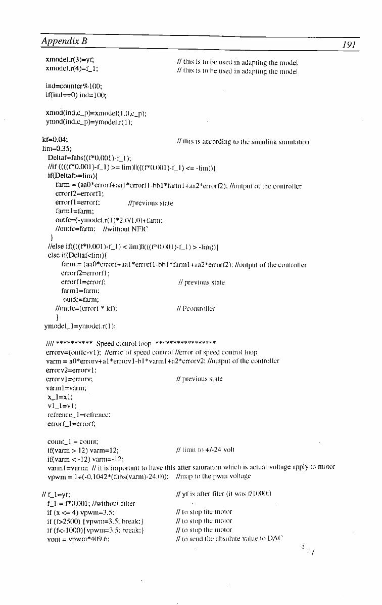
Appendix B jgj
xmodel.r(3)=yl; // tnis is t0 be used in atlapting the motlel xmodel.r(4)=l_l; // tnis is t0 b e used in .ldapti„g the m o d e l
ind=counter%100; if(ind==0)ind=100;
xmod(ind,c_p)=xmodel(1.0,c_p); ymod(ind,c_p)=ymodel .r( 1);
kl=0.04; // this is according to the simulink simulation lim=0.35;
Deltaf=fabs((f*0.001 )-f_l);
//if ((((f*0.001)-f_l) >= lim)ll(((f*0.<X)l)-f_l) <= -lim)){ if(Deltaf>=lim)(
farm = (aaO*errorf+aal*em)rfl-bbl*farml+aa2*errorf2): //output of the controller errorf2=errorf 1;
errorfl=errorf; //previous state farml=farm;
outfc=(-ymodel.r(l )*2.()/l .0)+farm: //outfc=farm; //without NFIC
1 //else if((((f*0.001)-f_l) < lim)ll(((f*0.<X>l)-f_l) > -lim)){ elseif(Deltaf<lim){
farm = (aa0*errorf+aal*errorfl-bbl*farml+aa2*errorf2); //output of the controller errorf2=errorf 1:
errorfl=errorf; // previous state farml=farm;
outfc=farm:
//outfc=(errorf * kf); // Pcontroller
} ymodel_l=y model.r(l):
//// ********** Soeed control loon *****************
errorv=(outfc-vl); //error of speed control //error of speed control loop varm = aO*errorv+al*errorvl-bl*varml+a2*errorv2: //output of the controller
errorv2=errorvl;
errorvl=errorv; //previous state
varml=varm;
x_l=xl;
vl_l=vl;
refrence_l =refrence:
errorf_l=errorf;
count_l = count; if(varm > 12) varm=12; // limit to +/-24 volt
if(varm < -12) varm=-12; varml=varm; // it is important to have this after saturation which is actual voltage apply to motor
v p w m = l+(-0.1042*(fabs(varm)-24.0)); //map to the p w m voltage
// f_l=yf; // yf is after filer (it was f/1000;)
f_l = f*0.001; //without filter
if (x <= 4) vpwm=3.5; // to stop the motor
if (f>2500) (vpwm=3.5; break:} // to stop the motor
if (f<-1000){vpwm=3.5; break:} // to stop the motor vout = vpwm*4()l».6; // to send the absolute value to D A C

Appendix B 192
if (varm < 0) vsign = 128*16; // to send the direction (1 = backward) else vsign = 0; // direction (0 = forward) da_out(l, vout); //0 to 10 calibrated
da_out(3, vsign); //should shift left 4 bits
da_out(2, vsign); //should shift left 4 bits end_timel =uclock();
exec_time = ((end_timel-end_time2)*1000.0)/l 103150;
if(exec_time < 10) delai=10.0 - exec_time;
else
delai = 0.0;
dela= (int)(delai+0.5);
delay(dela);
if (counter == 10000) break;
end_time2 = udockQ; loop_time=(end_time2-end_time21 )*1000.0/1193150.0; if (counter > 110) sampling_freq=l(X)0.0/loop_time;
fprintf(fp_in, "%t\t%f\t %f\t %t\t %t\\ '7< An".end_time2* 1000.0/1 lir3150,xl.vl,f/1000,yf,ymodel.r(l));
end_time2 l=end_time2; end_time2 = uclockQ;
prog_time =(end_time2-init_time)/l 193150.0; printf("Totaol Execution Time = %i [Sec] \t No. of Iteration = %d\n".prog_time. counter-KX));
//savemodl("mod32cln"); //save("m(xl42cln",&n()Sm_,&knVecti)rs_,&n()Knc)ts_,°rees_.&inDim_.&iiiV;irs_,\
// &c_,&initKn_,&initNo_.&traces_);
fclose(fp_in); while(l){ // to return the knife to its home position v p w m = 2 ; // to make it slower it should be 2.5:
vsign = 128*16; // backward direction
ad_in(l, &d_a[0]): ad_in(5, &d_a[l]); // position sensor
x=(-(d_a[l] - 4095)/16.25)-6.523077; f=(d_a[0]-2048)*5: // 5 is the calib. coeff. new scnsor[grf]
if(x<=3.5){ vpwm=3.5; //to stop the motor
vout = vpwm*40%/10;
da_out(l, vout): //() to 10 calibrated
da_out(3, vsign):
da_out(2, vsign);
exit(0):
vout = vpwm*409.6: // convert to send to DAC da_out(l,vout): //() to 10 calibrated
da_out(3, vsign); // should shift left 4 hits xpwm=2.5:
1 return 0;

Appendix B 193
B.3. A Sample Code to build an A S M O D model
ASMOD software which is written using 25 MATLAB functions can be used as
a main.m in MATLAB environment to build an ASMOD model. A sample code
for building a model is given below.
% main.m
load mine_test.dat; % load test data
load mine_train.dat; % load train data
xTest = [mine_test(:,l) mine_test(:,2) mine_test(:,3) mine_test(:,4)]; yTest = mine_test(:,5);
xTrain = [mine_train(:,l) mine_train(:,2) mine_train(:,3) mine_train(:,4)];
yTrain = mine_train(:,5);
degree=2; % the same spline degree (quadratic) is used for all variables %degree=[2 2 2 1 1 1 1 1 1 1 ] ; % individual spline degrees can be used
resolution=0; % the initial resolution (number of internal knots)
%resolution=[l 1 0 0 0 0 0 0 0 0]; % individual init. resol. can be used
initSubmodels = []; % Initialize as an empty model
% initSubmodels = [2 1 2; 1 3 0; 1 4 0; 1 5 ()]; % Initialize with % one 2 dimensional of variables 1 and 2, and three onedimensional
% submodels of variables 3, 4 and 5 respectively
xmin = D;xmax = []; % Automatic determination of input domain. % xmin = [000 0 0 0 0 0 0 0]; % Setting of input domain lower limits. % x m a x = [l 1 1 1 1 1 1 1 1 1]; % Setting of input domain upper limits.
iniAsmod(xTrain, degree, resolution, xmin, xmax.initSubmodels):
[traces, est] = train(xTrain, yTrain,xTest. yTest, 'SRM', 25);
%plot(traces(:,8), traces(:, 1:7)) [rmse, nrmse, ev, mae, maxe] = testModl(xTest, yTest)
saveModl( 'mine_model 1');

Appendix C:
PLASTIC CYLINDRICAL ANTI-PERSONNEL MINES
No.
1
2
3
4
5
6
7
8
9
10
11
12
13
14
15
16
17
18
19
20
21
22
23
24
25
26
27
28
29
30
31
32
33
34
35
36
37
38
39
40
Type
APNMAE TI
APNMM14
ARGES SPM75
AUPS
BM/85
BOOBYTRAPPED
CP-X.01
CP-X.02
DM-11
DM-39
FAMA
FMK-1
GYATA-64
K-2
LBA TYPE-A
LBA TYPE-B
LORY
M14
M412
MAI68
MAI75
MAI-GR1
MAI-GR2
MAP II
MAPP78 F-2
MAUS
MAUS PRACTICE
MAUS/1
MBV-78-A2
MD-82-B
MGP.30
MI AP DV56
MI AP DV59
MIAPDV61
MI AP DV M63
MIAPDVPIGX61
MI AP DV X59
MI AP ID 51
MN-79
NO.6
Weight
[KK1 0.42
0.10
6.00
0.30
2.00
0.39
0.085
0.078
0.231 -
0.086
0.2509
0.45
4.00
-
-
0.25
0.099
0.13
0.23
0.33
0.11
0.11
0.50
0.205
0.275
0.277
0.267
0.15
0.128
0.08-0.125
0.165
0.13
0.125
0.1
0.115
0.085
0.09
0.099
0.227
Diameter/Hight Min/Max [mm]
85 / 95
50 / 43
125/255
102-74/36
120/200
125/65
71/37
78/32
82 / 33.5
100/40
71/38
82-80/46.7
142- 106/61
100/225
108/33
108/33
115/40
56 / 40
88/32
78 / 68
95/61
75 / 45
70/45
113/83
-
89 / 46
89 / 46
89 / 46
53/ 130
55 / 55
90/40
70/78
62 / 55
35 / 270
35 / 270
54 / 274
60 / 32
70 / 52
56/40
40/200
Actuation
Force [KgfJ
17
9- 16
5 - 10 -
12- 13/6
7 - 30
14 - 36
14-36
5
-P1
30 -
7.5 -
-
-
15
9 - 16
5 - 20
15-32
5 - 25
-
-
10- 14
-
10
10
10.3
2-5
4-5
15
-
5
-
-
18
18
14-24
9.0 - 16.0
22.0
Burial Depth
Max/Min [cm] -
-
-
4.0 / 0.0 -
13.0/0.0 -
-
-
-
-
-
10.0/0.0 j
20.0/13.0
6.0 / 3.0
6.0 / 3.0 !
6.0 / 0.0
-
-
-
-
-
-
-
I
4.0 / 0.0 !
4.0 / 0.0
4.0/0.0
-
-
-
- / 8.0
-/0.0
-
-
-
-
50 / 0.0
-
1 Pressure Release

Appendix C
No.
41
42
43
44
45
46
47
48
49
50
51
52
53
54
55
56
57
58
59
60
61
62
63
64
65
66
67
68
69
70
71
72
73
74
75
76
77
78
79
80
81
82
83
84
85
86
87
Type
NR22
NR22C1
P5
P-4-A
P-4-B
P-40
P2MK2
P4MK1
PATVAG 59
PATVAG M3
PM79
PMA-2
PMA-3
PMN
PMN-2
PMN-4
PMP71
POMD-1
PP MI-SR
PP MI-SR II
PPM-2
PRBBAC H-28
PRB M35
PRB M409
R2M1
R2M2
T-AB-1
T/79
TM-100
TRUPPMINA 10
TYPE 58
TYPE 63
TYPE 68
TYPE 72
TYPE 72A
TYPE 72 B
TYPE 72C
U/I
U/ITH(AP.l)
U/I TH (AP.2)
UNKNOWN
UNKNOWN
VALMARA 69
VAR/40
VSAPFM1
VS-MK2-EL
ZAPS
Weight
[Kgi
0.085
0.13
0.13
0.21
0.171
2.00
0.14
0.095
-
0.095
0.28
0.135
0.183
0.55
0.417
0.3
1.0- 1.5
2.7
3.2
3.2
0.39
0.165
0.158
0.183
0.13
0.128
0.125
0.19
-
0.231
0.55
1.335
2.8
0.14
1.00
0.15
0.28
0.013
0.13 -
0.206
0.13
3.3
0.1
3.5
0.2
1.7
Diameter/Hight Min/Max [mm]
70 / 52
62 / 55
88/32
72 / 55
73 / 43
90/215
70 / 38
72/45
71.9/52.8
79/18
88.0/48.0
68.0/61 & 3 0
103/36
112/56
50.9- 121.2 / 52.3
46 / 95
175/115
112/135
102 / 152
102 / 152
81.8- 124.7/63
90 / 28
63.5/39.0
82/28
69 / 57
69 / 57
60/61
-/45
33/ 107
80.5-79.8/33.5
112 / 56
140/ 190
135/109
78.5 / 38.5
64/123
78.5 / 38.5
78.5 / 38.5
44.5/15.0
100/40
80/40
81 / 35.5
28/ 150
130- 107/205
78/45
130/190
89.5 / 35
90/210
Actuation
Force [Kgf]
5.0 -25.0
5.0
5.0 - 20.0 _
10.0- 14.0
7.0- 13.0
10.0
10.0
5.0
15.0
5.0 - 25.0
5.0- 15.0
3.0- 15.0
8.0-25.0
15.0
2.0- 15.0
6.0
-T2
4 - 8 / 3 - 6
4 - 8 / 3 - 6
12.5
9- 19
9- 14
8 - 30
1 -6
3-7
15 -
Varies
10
-
-
7-20
5-7P
7 - 20 P
3-7P
2.5 - 25 P
2.5 P
-P
-P
5 - 20 P
-P
10 P
12-13
6.3 T
-P
C3P
Burial Depth
Max/Min [cm] _
.
_
:
_
_,
_,
_
10.0/0.0
5.0 / 0.0 j
9.0 / 0.0
8.0/0.0
25.0 / 0.0 _
.
9.0/4.0 !
.
20.0 / 0.0
20.0 / 0.0 |
10.0/0.0 -
-
-
-
-
-
-
3.3/0.3
3.0 / 0.0
25.0 / 0.0 -
-
8.0 / 0.0
18.0/0.0
8.0/0.0 :
8.0 / 0.0
2.0 / 0.0
-
-
12.0/0.0
19.0/0.0
17.0/12.0
-
-
2.0 / 0.0
-
2 Trip Wire 3 Command Initiation