B.A.H.C-1420

oo

DATA BASE PERTINENT TO EARTHQUAKE DESIGN BASIS

by

R. D. SharmaSeismology Section

1988

B.A.R.C. - 1420

GOVERNMENT Of-' INIJiAATOMIC ENERGY COMMISSION

of<CD

DATA BASE PLH 11NENT TO EARTHQUAKE DESIGN BASIS

by

R.,D. ShannaSeismology Section

BHABHA ATOMIC RESEARCI-! CENTREBOMBAY, INDIA

1988

A C K N O W L E D G E M E N T S

This document has relied, particularly for the geologi-

cal aspects of the earthquake problem, on published

literature, which has been duly acknowledged in the text.

The benefit derived from a course on the Earthquake Aspects

of Siting Nuclear Power Plants, organised by the Interna-

tional Atomic Energy Agency and the Argonne National

Laboratory Chicago,U.S.A. is gratefully acknowledged. I have

also benefitted from interaction with Mr.D.C.Banerjee of the

Atomic Minerals Division, Department of Atomic Energy,

Mr.A.Kakodkar and Dr. A.K.Ghosh of the Bhabha Atomic Re-

search Centre and Mr.V.Ramachandran and Mr.U.S.P.Verma of

the Nuclear Power Corporation. I am grateful to

Dr.G.S.Murty, Head Seismology Section for his interest in

this work, and for critically reading the manujscript.

of

1. INTRODUCTION 1

2. APPROACH TO BEXSMIC RISK ASSESSMENT. 2

3. ASSESSING SFrc " ' /:r7OiMIC STATUS OF THE SITE REGION. . . .5

3.1. AbGOo:.AT::Kfc EARTHQUAKES WITH KNOWN FAULTS 6

3.2. INVESTIGATING FAULTS 8

3. 2. I.. INTERPRETATIONS FROM REMOTE SENSING DATA. 12

3.2.2. DATA ON PREHISTORICAI* EARTHQUAKES 17

4. MICROEARTHQUAKE STUDIES 18

5. EARTHQUAKE' DA** AMD TECTONIC STRUCTURES 19

6 . INDUCED SEISM.iCITy 22

6.1. CAUSES OF .rtJyEKVOiK INDUCED EARTHQUAKES 23

6.2. IDENTIFY : ,••.-• SIS EARTHQUAKES 24

7. EVALUATING MAXIMUM CREDIBLE EARTHQUAKE ON A FAULT 27

8. ATTENUATION LAWS FOR GROUND MOTIONS 28

9 . STRONG MOTION DATA .35

9.1. EARTHQUAKE RESPONSE SPECTRA. 36

9.2. SPECIFYING EARTHQUAKE RESPONSE SPECTRA 38

9.2.1. STANDARD RESPONSE SPECTRA 39

9.2.2. USE OF GROUND MOTION AMPLIFICATION 42

FACTORS

9.3. SITE-SPECIFIC SPECTRA 43

10. ROLE OF LOCAL GROUND CONDITIONS 44

11. NONLINEAR BEHAVIOUR OF STRUCTURES 46

12. CONCLUSIONS 47

13. REFERENCES 48

DATA BASE FEBTIHEMT TO EARTBQOAKE DESIGN BASIS

by

R.D.Sharma

1. INTROPUCTIOH

Mitigation of earthquake risk from impending strong

earthquakes is possible provided the hazard can be assessed,

and translated into appropriate design inputs. This requires

defining the seismic risk problem, isolating the risk fac-

tors and quantifying risk in terms of physical parameters,

which are suitable for application in design. Like all other

geological phenomena, past earthquakes hold the key to the

understanding of future ones. The seismic risk problem in

the context of engineering design encompasses the following:

(i) Estimating locations and strengths of future

earthquakes resulting from slippage along faults,

(ii) Assessing their effects at a site as a result of

possible shaking and ground failure phenomena,

(iii) Estimating the probability of the ground motion

exceeding a certain specified value during one

single event.

(iv) Estimating the probability of the maximum slip

during a specified period, say the operating life

of a nuclear power plant,

(v) Quantifying the resulting ground movement at the

site following any earthquake.

Quantification of seismic risk at a site calls for in-

vestigating the earthquake aspects of the site region and

building a data base. Th3 scope of such investigations is

illustrated in Figures 1 and 2. A more detailed definition

of the earthquake problem in engineering design is given

elsewhere (Sharma,1987). The present document discusses the

earthquake data base, which is required to support a seismic

risk evaluation programme, in the context of the existing

state of the art.

2. APPROACH TO SEISMIC RISK ASSESSMENT

For the aseismic design of nuclear power plants, col-

lecting information on past earthquakes (see Figure 3),

which have occurred within 300 kilometers of the site, has

been recommended (U.S.N.R.C.,1980) Epicentres of past

earthquakes are superimposed on a plot of lineaments/faults

of the region on a 1:1000,000 scale map, as accurattjy as

possible. (Plotting these data is so carried out that mag-

nitudes of the earthquakes and their number in a specified

grid can be assessed from the plot). It is desirable that

for the earthquakes plotted on one map, accuracy of

epicentral locations and magnitude determinations is

comparable. If the entire data set is not of uniform ac-

curacy it is preferable to prepare more than one map, so

that each map contains data of comparable quality. These

maps are, then, supplemented with the geological map of the

region. After the preliminary seismotectonic and geological

information is compiled, one proceeds to:

(i) Divide the 300 km radius area into tectonic

provinces (see USNRC,1980).

(ii) Identify significant tectonic features

(lineaments, which could be considered or

suspected to be the surface expressions of

(iii) Associate as many earthquakes as possible with

Luown tectonic structure.

(iv) Estimate occurrence rates (in time and space) of

earthquakes of different magnitudes associated

with each tectonic structure (or province),

(v) Estimate the maximum earthquake potential of each

known tectonic structure (or province).

(vi) Identify the earthquakes which cannot be as-

sociated with known tectonic structures.

(vii) Investigate the area through landsat imageries,

aerial photographs, detailed geological maps and

ground truth verification to determine if addi-

tional tectonic structures, which could be con-

sidered the sources of the unidentified

earthquakes, could be found, and (if they existed)

establish their geological characteristics,

(viii) Set up an attenuation law for each source-site

combination to translate earthquake effects into

vibratory ground motions at the site.

(ix) Select a methodology through which values of

acceleration, velocity and displacement from fu-

ture earthquakes could be estimated.

(x) Set up a model through which the influence of the

local geology in modifying the the base ground mo-

tions at the site may be characterized.

(xi) Determine the difference between free field

motions and those due to the presence of the fu-

ture and existing engineering structures at or

near the site to arrive at the design basis ground

motion estimates.

In aseismic design the importance of the informet.iun •;•

regional geology and tectonics on the one hand and iack of.

such information in most regions of the world on the other

cannot be overemphasized. In some regions, which were

believed to be earthquake free on the basis of such in-

adequate information, faults were discovered after su

.; ;a \'.iquake occurred. By now, it has become abundantly clear

that, unless investigations have been carried out to seek

evidence against existence of geological faults, lack of

reported evidence cannot become the basis to infer low seis-

mic risk. These investigations are elaborate and time

consuming. Only well organized efforts in data acquisition,

pursued for several years before a site is considered for

constructing a. nuclear power plant, can produce the desired

results. A practical approach would be to identify probable

areas of development, and study them in detail, sufficiently

in advance to build the data base.

3. ASSESSING SEISMOTECTONIC STATUS OF Till'.: jilll

Earthquake hazard in a r- •:.. ••. . • J several fac-

tors associated witii geological f-au.; ..-., .1 - ,. •., ;r.,. •„ history

of the region (see Figure 4). Scn-r rH-.. !•* u «iaj j-oduce

earthquakes whereas others may be ar-i'- ""v-•* > ^iMi-,t,. It i =

also possible that a fault is untie r-., i r-<- i—.-Jasti'j rro r .• -

(creep), and generating no earthquak«-j. in 3 ->*=i5.m.ie

fault has been called a capable f au'i i, if . 1.1 .. ha>\

nificant potential for relative d',.,, , ., •, • .. , -

ground surface (IAEA, 1979). Earthquake h&_: ,.•.'. fro:/, --.

fault is determined by the strongest, tj i ti< \ ..-,, - ;•:-[• • :JX-

imum aseismic creep), which can be assoo.i &Leu with a fault.

For assessing seismic risk associate;; W;LL.:. .-A .. or,jtructio;/

site, all faults exceeding a couple of hwndied meters length

need be evaluated separately ror asaessing their

earthquake/creep potential. For tbl:-; >across tae ,. :.-'.•;,*;'•:.

seismicity and geological maps of the area are to be ex-

amined in conjunction with other available information from

remote sensing and geological field •itd i.e. determine i^

earthquakes have occurred in the region, ami could be as-

sociated with known faults, or t;vi.H;> . . r ieiat.:ve move-

ments along the fault could be infei. .J.

3.1. ASSOCIATING EARTHQUAKES WITH KHOWN FAPLTS

Earthquake epicentres, when plotted on a tectonic map,

rarely lie along the lineaments of known faults. This

results from several factors, e.g. inaccuracy in the

hypocentral location, a less accurately defined fault

lineament, branching along the fault and dipping of the

fault surface away from the vertical. Associating the ob-

served seismic activity with known faults is a difficult,

but important step in specifying earthquake design basis. An

earthquake which cannot be associated with any known fault

has been called a floating earthquake, and has to be treated

differently. Associating earthquakes with faults is a matter

of interpretation, accuracy of which depends on the avail-

able information on the earthquake source and the geological

structure. From design point of view, the interpretation

leading to the worst possible event (from safety point of

view) is examined. The following steps may be helpful in : s-

sociating epicentres of earthquakes with known faults.

1. The earthquake should be located as accurately as

possible (say, epicentre within 1 km and depth

within 5 km). The earthquake may be considered as-

sociated with the known fault if, within the ac-

curacy of the earthquake source location and the

definition of the fault lineament, the earthquake

source may be considered close enough to the fault.

2. If earthquake effects are observable, the isoseis-

mals will be elongated almost parallel to the

fault, at least in an area close to the epicentre,

if the earthquake was associated with the fault.

3. It is believed that earthquakes occur to fill the

gaps (Mogi,1979). Supporting evidence in the form

of occurrence of other earthquakes along the fault,

including aftershocks and foreshocks, may be sought

from the earthquake history of the region.

4. If the earthquake in question is of post instrume-

ntal period, and has been recorded at a suffi-

ciently large number of stations (say,ov^_ .• .ic.:en)

a fault plane solution may allow the determination

of the strike and dip parameters of the causative

fault.

5. Fault dimensions should be consistent with the

magnitude of the earthquake(see Table I).

It is not uncommon to encounter situations i1-. siting

when epicentres in the site region cannot be associi..,ed v.ith

any known geological structure. In such cases the region

around the site requires to be investigated further in

detail. If the area is examined through enhanced landsat, im-

ageries supplemented by aerial photographs and field checks,

the possibility of a lineament being revealed close to the

earthquake in question is not ruled out. A microearthquake

network enclosing the epicentres of these earthquakes is

likely to be helpful in delineating the lineament par-

ticularly in the case of a burried fault(IAEA,1985).

3.2. INVESTIGATING FADLTS

On the basis of historical earthquake data some areas

are considered free from earthquakes, implying a seismically

stable region. However, the duration of reliable historical

records of earthquakes is much too short to ensure such

stability in times to come. Recurrence intervals of strong

earthquakes (which could be felt or, which would have left

on the ground any apparent evidence of their occurrence) are

often longer than the total span of the recorded history of

earthquakes. Complete absence of earthquakes in a region

cannot be established unless a sensitive network of seis-

mographs has been operating in the area for many years. It

is, then, desirable to look for evidence of fault capability

using seismic monitoring and, side by side, geophysical

techniques based on data from remote sensing, geological

mapping and field geology. Regional tectonics can be studied

by investigating ground lithology and stratigraphy, and

using remote sensing data, such as available from Landsat

imageries, aerial photographs, aeromagnetic data,

aeroradioactivity data etc.

In investigating a fault, the first and the foremost

requirement is to establish that it really exists. A map

containing lineaments picked up from Landsat imageries and

epicentral locations of well located earthquakes is helpful

in achieving this objective. If earthquakes, which have oc-

curred in the region under investigation, are accurately

located, the epicentres will lie close to the strike of a

vertical fault. If a fault plane solution is available ':-..

the earthquake, directions of strike, dip etc. will ,.150 l~

known. (A fault plane solution will be possible only if data

from a set of seismic stations on both sides of the fault,

are available). If a reasonably good number of well located

earthquakes is not available for the region, seismic

monitoring using modern sensitive seismographs to alxow

location of microearthquakes and analysis of waveforms

should be undertaken to upgrade the data base. As a result

of loose coupling of the ground along the . • . L -. .

waves are likely to be anomalously attenuated whilt ra/spa-

ing the fault zone. Geological field studies on the fault,

where it is well exposed, may provide information on the ex-

tent and age of fault movements. Stratigraphic obosrvatior:

on two sides of the fault may reveal the movement along the

fault. It may be possible to determine the rate of movement

by dating the strata on two sides of the fault.

Identification of a fault and assessment ox it?

earthquake potential call for detailed surface and subsur-

face investigations to determine fault dimensions and

extent, nature and history of movements associated with past

earthquakes (or aseismic creep). Evaluation of fault

capability requires estimating:

a. the probability of slip during a specified time

interval, say the life time of the engineering

structures, and

b. the probability of a certain specified slip being

exceeded during a single earthquake.

For estimating these probabilities reasonably ac-

curately information on the history and source mechanisms of

past movements is required (see Cluff et al.,1980;

Coppersmith, 1981). In engineering design a fault is con-

sidered capable if it has shown (see IAEA,1979; USNRC.1980):

1. Evidence of movements, at least once, in the past

35,000 years, or movements of recurring nature at

or near the surface within the past 500,000 years,

such that the possibility of further movements can

be inferred.

2. Structural relationship to a known capable fault

such that movements on one may cause movements on

the other at or near the surface.

3. Macroseismicity instrumentally determined with

records of sufficient precision to demonstrate a

direct relationship with the fault.

Surface and subsurface details provide evidence for (or

against) significant faulting at or near the surface (see

Figure 5). If faulting is present, determining the

direction, extent and age of movements is an important com-

ponent of determining fault capability. Geomorphic features

are particularly useful in determining the age of the

movements. When faulting is known or suspected, investiga-

10

tions using stratigraphic and topographic studies, surface

survey, trenching and other techniques have the potential of

providing detailed information on fault movement. Consider-

ing the uncertainties in the results of the various geologi-

cal techniques it is desirable that as many of the several

methods as possible for studying fault movements, e.g.

structural superposition, geomorphological and

geochronological methods are applied. If topographic fea-

tures shown on photographs, or inferred from other remote

sensing data, are investigated in sufficient detail to ex-

plain their causes, or to establish lack of any possible

jjwoiitfgieHi t>#ua«, fairly detailed information on fault

capability c^n emerge. Sites in regions of complex geology,

or high .'jeismicity, require more detailed investigations.

Depending on the geological conditions of the site and its

vicinity, subsurface geological and geophysical investiga-

tions using bore hole geophysical techniques, gravity and

magnetic surveys and seismic techniques, test excavations,

shafts, trenches and tunnels yield information on surface

faulting. In the absence of a surficial evidence, examina-

tion of a geological profile in a test trench may prove very

useful. The trench walls may provide evidence for (or

against) fault capability. The purpose of investigations in

a trench is to determine whether surface deposits lying

across tho fault are displaced (see Clark et al.,1972).

Evidence of large prehistoric earthquakes can be found by

examining the sedimentary deposits in the structures, which

could have been preserved following strong earthquakes.

11

Remote sensing data are useful in delineating a fault, as-

sessing its activity level and determining fault type and

fault length (McEldowney and Pascucci,1979). A discontinuity

in lithology, vegetation, ground moisture, thermal

properties, texture, colour, stream pattern and topography

across a lineament can lead to fault detection. A study of

mioroearthquakes recorded over a reasonably good interval

(upto a period of three years in a moderately active area)

can also be helpful in identifying the fault (IAEA,1985).

Large scale low sun angle photographs are useful in iden-

tifying fault scarps. In conjunction with fracture density

mapping and ground studies they allow detection of increase

in fracture density, thereby determining the projection of a

fault, and the displacement near the faulted zone.

All faults measuring over a few hundred meters in

length at or near the site should be investigated. In some

areas dormant faults might have been reactivated by large

reservoirs due to water loading or fluid injection (see Sec-

tion 6). Some investigations of the type mentioned above

would provide evidence in favour of, or against, recent

fault movement.

JLJLX,., INTERPRETATIONS FROM REBOTS SENSING DATA

Application of Landsat imageries and aerial photographs

has proved very useful in investigating geological faults at

moderate costs, both in terms of time and money. Landsat im-

agery offers a broad overview of the site at low sun angle

12

elevations permitting observation of the entire area of in-

terest for examining structural patterns, accentuating minor

differences in topography and vegetation. They allow iden-

tification of lineaments, which are the surface expressions

of faults and fractures, and are helpful in determining the

extensions of known faults (see Zall and Michael,1980).

Landsat imagery contains the response of the earth's surface

to radiation in the 0.5 to 1.1 micrometer wave length range,

i.e. the visible and the infrared, in four distinct bands

(0.5-0.6 um, 0.6-0.7 urn , 0.7-0.8 um and 0.8-1.1 nm) in

185km x 79m strips on the earth surface. The spatis.1 .-esc..,:-

tion of the imagery from multispectral scanner XL 7-.' - . !; JS

and can be enhanced to 55 metres by computer p.-c 'sssing.

Colour composite images, which are produced from data in

more than one band, offer increased interpretability of the

image. Twenty percent of each Landsat image can be viewed

stereoscopically. They are available at scales of

1:1000,000, 1:500,000 and 1:250,000. These data are avail-

able with the National Remote Sensing Agency (f« oA) at

Hyderabad in digital form on computer compatible tapes

(CCT), using which much higher resolution can be obtained.

Recognition of faults on an imagery picture requires

locating discontinuities or changes across the surface in

terms of the alignment of features along the strike. Dis-

placements along faults brings into juxtaposition features

of different rock types. Differences in their physical or

botanical properties, if detected using appropriate type of

imageries, enable identification of the fault contact.

13

Variations in lithology, vegetation, ground moisture and

topography, can be deteoted on imageries. Rock units having

differences in reflectance (colour) may readily be distin-

guished on imagery. The texture and overall pattern of rock

masses are usually more useful in distinguishing rock types

and boundary faults. The dominant textural component of rock

masses from imagery standpoint is the texture associated

with the stream (or drainage) pattern. Rock mass structure

and hardness are refleoted in the pattern and density of the

drainage system. Changes in pattern, density or texture of

the stream pattern often denote a contact between fault

surfaces. Thermal properties of rooks may provide useful

contrast when imagery equipment is sensitive to radiation in

the appropriate thermal range. For example, thermal inertia

may vary between two different rock types having the same

colour and brightness in day time. A thermal scan at night

may show one rock type warmer than the other. Faults occur-

ring within a single rock unit are usually indistinguishable

using rock reflectanoe or texture alone. Different rock or

soil types may support different plant assemblages, or a

particular plant assemblage may exhibit variation in growth

characteristics, e.g. age, vigor, density etc. Variation in

vegetation may occur as tone contrast across a fault, which

is generally due to differences in the type of vegetation on

the two sides of the fault. Vegetation contrast may also oc-

cur as texture oontrast across a fault due to changes in

type and density of vegetation. Difference in moisture may

give rise to denser growth on one side of the fault. A fault

14

may serve conduit for fluid flow promoting vegetal growth

along the fault and associated fractures. The moisture dis-

continuity may result in measurable changes in ground tem-

perature (due to evaporation) and changes in reflectance of

the soils on opposite sides of a fault. Ponding may also oc-

cur along the trace of a fault forming a string of "sag"

ponds. Vegetation along fault scarps (steepened land

surfaces, which are more definite indicators of faulting)

may be younger than that on either side of the fault. Im-

agery in the near infrared region is required for inves-

tigating variations in vegetation, since planx, x cie.t.iri ^

in this region is a function of plant heaiui. ua leaf

texture. Plants under stress exhibit a lower reflectance in

the infrared compared to the healthy ones, even though the

reflectance in.the green region (due to chlorophyll) may not

show much variation. Plant stress may be caused ei'.,.,er by-

lack of moisture or toxic fluids flowing along the fault

fracture. Acive faults may also form a barrier to the free

flow of water through near surface materials. Fault scarps

may often be detected in materials of uniform mineralogy,

surface texture or moisture conditions, simply because one

side of the fault is closer to the sensor.

Aerial photographs can show some of those features of a

fault which cannot be found directly by ground studies.

Their use provides a resolution of as much as 1 metre on the

ground surface (Babcock, 1971; Colwell, 1961; Reeves et

al.,1975). Most pcirt of the country has been photographed at

1:25,000/1:50,000 scale. Photographs of different dates are

15

vailable in the depository of the Survey of India. These

can be used to study temporal changes in superficial and

!ectonic features. Aerial photographs allow stereoscopic

•'iewing, thus enabling detailed observations on fault

xeatures. A major difficulty in using aerial photographs

arises from the procedures, which have to be followed in

letting access to the photographs. (As per the existing

rules, investigators have to individually seek permission

xrom the ministry of defense. Examination of photographs is

'•,o be carried out in the depository of the Survey of India.

Defense clearance takes considerable time. The rules e;.3'

lay restrictions on making notes and sketches from the

photographs.)

Detailed examination of Landsat imageries and aerial

photographs is to be followed by ground truth verification,

i.e. field checks to identify some of the observed features

on the ground. Features which can be helpful in recognizing

active faults are given in Figure 5 (see Slemmons,1977). I.

an active fault has been encountered, a combination of some

of these features may be detected during field checks.

Stratigraphic offset of Holocene or late Quaternary soils,

and sediments are common. Unusual variations in

atratigraphic thickness or sequence across a fault zone may

be present. Fault creep may be shown by offset fences,

highways, roads, walls, buildings etc., or by geological

displacements or distortions at or along fault zones.

16

3.2.2. gATA QN P^EHtSTQR^CA^ gARTHQOAKKS

Historical and instrumental data on earthquakes contain

ample evidence to demonstrate that locations, magnitudes and

frequencies of earthquakes are not entirely of random

nature. Several factors influence earthquake occurrence in a

region, e.g. the rate of strain accumulation, the area of

•the strained region, the shearing resistance along the

fault, the amount of sudden fault displacement, the size of

the most recent earthquake and the time elapsed since then.

These conditions vary from fault to fault, and so varies the

probability of earthquake occurrence, their magnitudes and

locations. Since earthquakes result from a gradual process

of strain accumulation followed by a sudden release of

energy, the spatial and temporal distribution of past

earthquakes is the key to understanding the earthquake

process in a region. Existing data on large earthquakes are

too few (and the earthquake mechanism too obscure) to allow

modelling of the earthquake process purely on the basis of

these data. The size of the data sample of strong

earthquakes can be considerably increased using the

geological evidence of past earthquakes obtained from

trenches across fault traces. It is possible to find

evidence of faulting from strong earthquakes of prehistori-

cal times (Bonilia et al.,1978; Seigh, 1978). Estimating the

frequencies of fault displacements on the basis of geologi-

cal evidence require;; a knowledge of the age of the faulted

17

block and "the ages of "the yo.u^ge^ strata. The

investigations, which are used to ge:J;hsr j/iforaiat-i.cn on

earthquakes occurred in prehistoric^ J :. \-.~sz £..-.'. 1 '":.thir; the

purview of Quaternary geology,

4. MICKOKARTHQOAKE STUDIES

A microearthquake survey using a saix.ftfaiy planned net-

work can provide good insight into the seismotectonic status

of a region. Analysis of microearthquake data can provide

quantitative information on several aspects of earthquake

sourci . in the region, e.g. their aisc i e.ibit,; ieioaao,

dimensions of the rupture), geometry of che vault (extent of

faulting, direction of strike and sense of slip), nature of

faulting, dynamic properties of the source region (average

displacement across the fault, rupture propagation velocity,

stress drop), regional seismic velocity structure, elastic

constants, seismic signal attenuation and energy transfer

characteristics of the site region. ucij.ix.y of

microearxhquake data is dependent on the accuracy of source

locations, and that of the information collected from the

analysis of signal waveforms. Absence of microeai-thquakes in

an area cannot serve, by itself, as a proof against fault

activity. To make full use of thest; •:•.*-:.,- .: .-or::. j ed ,i=o logi-

cal information pertaining to the , -r-...'. j;. ;onic movements

should be collected from remoce sensing data, ground checks,

gravity and magnetic anomalies and basement topography, and

integrated with the microearthquake data. A study of

18

microearthquakes recorded over a period of about- three years

has been recommended for identifying faults and their ac-

tivity levels in a moderately seismic area (IAEA,1985). Ac-

curate location of microearthquakes may lead to the dis-

covery of potential seismic zones, which may later on be

mapped using suitable geophysical techniques. The data from

A microearthquake survey will also provide a basis for

treating floating earthquakes (the ones which cannot be as-

sociated with any known fault and, for the purpose of aseis-

mic design, are considered equally likely to occur anywhere

in a region). In case of these earthquakes, one is fscsc!

with the problem of determining a certain distance from the

site within which the probability of earthquake occurrence

may be considered very low (see IAEA,1979). This can be en-

sured by demonstrating through microearthquake survey that

no geological structure capable of producing an earthquake,

which could be considered of any engineering consequence,

exists within a certain minimum distance from the site. A

detailed account of the current state of the art in

microearthquake recording and data analysis has been given

by Lee and Stewart (1981). The I.A.E.A. document (IAEA,1985)

provides guidelines for conducting a microearthquake survey

around a nuclear power plant site.

5. EARTHQUAKE DATA AMD TECTOHIC STROCTURES

Earthquake occurrence in different parts of the globe

has shown two important characteristics, namely:

19

(a) Earthquakes follow a magnitude frequency-

relationship, namely fewer the larger

(Richter,1958).

(b) Earthquakes often occur to fill gaps (Mogi,19?9).

Implications of x.hsse characteristics are: (i) an area

where smaller earthcuaiies have occurred in recent times

could be affected by strong earthquakes in future, i'iii an

apparently seismically quiet area may be passing through a

seismic gap, aijd could be affected by a strong earthquake ir»

the near future. The effect of an earthquake on an engineer-

ing structure at a given site depends a great desl en —

location of the earthquake source with respect to tke ..• J ' .

Based on the seismotectonic history of the reg.lrc ;

probability event has to be defined in terms of ground mo-

tion at the site at different frequencies. This requires

that the magnitude distribution in the earthquake population

in the region (both in time and space) is estimated

reasonably accurately. Detailed seismotectonic maps to iden-

tify earthquakes (associating them with known tectonic

structures) are not yet available for most regions of the

world, largely because the inadequacy in the quality and

quantity of the available earthquake data.

A computer compatible data file containing magnitudes,

hypocentral locations and origin times cf I diaii earthquakes

obtained from national and international networks an<5 other

published catalogues is now available for use in earthquake

risk assessment. A summary of these data for th<* Indian

subcontinent for the post instrumental period in. terras of

20

the frequencies of earthquakes of different magnitudes for

10 degree squares are given in Table V (see Figure-6). As-

suming that earthquakes follow a magnitude frequency

relationship of the type

LogioN(M) = a - bM (1)

where N(M) is the number of earthquakes occurring annually

in an area, and having magnitude greater than or equal to M,

the estimated values of the parameters a and b are also

given for each square in this table. The a and b estimates

may not be considered representative for the entire area in

a square, as the squares in Figure 6 are not geologically

contiguous areas (so as to constitute what is called a tec-

tonic province). Secondly, there are limitations of the

regression analysis, particularly with inadequate data.

Paucity of data for some regions may be either because the

region is relatively free from earthquakes or because a

seismograph network, which is sufficiently sensitive to

detect small earthquakes, does not exist in the region.

Numerous earthquakes having magnitudes less than 4 have been

recorded by the Gauribidanur array (GBA), since it started

operating in 1965 in an area, which had usually been con-

sidered practically aseismic (Sharma and Murty,1973; Var-

ghese et al.,1979, Gangrade et al.,1987). A dense network of

sensitive seismographs is. therefore. a necessity in a

region where seismicity is important in engineering design.

Only after such a network has operated for a sufficiently

21

long interval (say. three years). the earthquake status of

the region could be assessed with some confidence. Inter-

pretations on seismic risk during a short monitoring

program, if few earthquake signals are recorded, can be

meaningful only if absence of potential earthquake sources

in the region can be established through detailed geological

investigations. A fault having the potential of a large im-

pending earthquake does not necessarily produce a propor-

tionate number of smaller earthquakes. It is also possible

that the fault is passing through a seismic gap, and absence

of recorded earthquakes may be an indicator of a strong

earthquake, sometime, in future.

g. JWPPCKP SfiiaHCITY

Tectonic earthquakes result from slippage of large rock

masses along faults due to strain accumulation beyond their

bearing capacity. In areas of critically stressed fault

zones, earthquakes may be induced by a slight increase in

stress Cor change in stress distribution) due to external

causes, e.g. impoundment of a large reservoir, injection or

extraction of fluid and mining activity. Among the several

causes of induced seismicity, impoundment of reservoirs has

drawn maximum attention. The issue whether the earthquakes

in Koyna region were induced by the reservoir was debated

for several years. In areas under development controversies

tend to arise, and are difficult to settle, when the seismic

history of the region under consideration is not well

22

documented. It is, therefore, desirable that steps to col-

lect earthquake data from such regions are taken much in ad-

vance of impounding a reservoir, or beginning any construc-

tion activity. This will be helpful in arriving at the

earthquake design basis in an objective manner. During the

post construction period precautionary measures could be

taken, if tremors suddenly start occurring while the criti-

cal facility is operating, on the basis of the collected

information. Despite the attention paid to understand the

nature and causes of reservoir induced seismicity, its ex-

planations remain largely conjectural. A detailed account of

the present status and future possibilities in this area has

been given by Gupta and Rastogi (1976).

6.1. CAUSES OF RESERVOIR INDPCED KARTHQDAKES

Several explanations have been extended for the ob-

served reservoir induced seismicity (RIS), namely:

(a) Sagging of the reservoir basin due to water loading

and consequent readjustments of the underlying sub-

stratum reactivating pre-existing faults.

(b) The added stresses due to water loading, triggering

the critically stressed pre-existing faults.

(c) Increase in pore pressure resulting in a decrease in

the effective stress, and increase in the ratio of

shear to normal effective stress. If rocks are under

initial stress, an increase in fluid pressure can

cause earthquakes. (The shear strength of rocks is

23

related to the ratio of the shear stress along the

fault to the normal effective stress, which is equal

to normal stress minus the pore pressure),

(d) The existing stress fields may be disturbed due to

entry of cold water into warm rocks.

RIS has not been observed in all reservoirs. Some con-

ditions have been identified for the occurrence of RIS. It

is believed that RIS is likely to appear if the following

conditions are fulfilled, all at the same time,

(i) A fault exists beneath the reservoir,

(ii) The basement consists of competent strata,

(iii) Large ambient stress differences exist in a

critically stressed medium,

(iv) Background seismicity is low. High background

seismicity renders the possible trigger effects of

the reservoir ineffective.

The height of the water column, the rate of change in

water level, the duration for which high water levels are

retained etc. are some factors which are likely to influence

occurrence of RIS earthquakes.

6.2. IDENTIFYING RIS KARTHQDAKES

Several parameters have been suggested for identifying

RIS earthquakes. These include:

(a) The slope of the magnitude frequency linear

24

relationship (Equation 1).

(b) Ratio of the magnitude of the largest aftershock to

that of the main shock,

(c) Foreshock-aftershock pattern, and

(d) Time distribution of the foreshocks and aftershocks.

Like regular earthquakes, those arising from RIS are also

observed to follow a magnitude frequency relation of the

type of Equation 1, with b values relatively higher than

those observed in case of normal earthquakes. In normal

earthquakes, aftershocks are characterized by b values

higher than those of the aftershocks. This relationship is

reversed in the case of RIS earthquakes. Another criterion,

which has been identified to discriminate RIS earthquakes

from normal ones, is based on the difference in their tem-

poral distribution patterns. Three distinctly different pat-

terns have been observed in an earthquake sequence. These

have been named as Type I,II and III patterns respectively.

In the Type I pattern the earthquake occurs without sig-

nificant foreshock activity, but it is followed hy a large

number of aftershocks. This is characteristic of a uniformly

distributed stress acting in a homogeneous medium. When the

material is heterogeneous and/or the applied stress is not

uniform, small foreshocks occur before the main shock, which

is followed by a number of aftershocks. This pattern is

called Type II pattern. The Type III pattern occurs when the

material is extremely heterogeneous and/or the applied

stress is concentrated over a small area. Here a swarm of

25

earthquakes occurs. The three patterns are illustrated in

Figure 7. The number of shocks and their magnitudes first

gradually increase and then decrease after some time. It has

been observed that the normal earthquakes in the Koyna

region belong to Type I while the RIS earthquakes show Type

II patterns. A comparison between the magnitudes of the main

shock and the aftershocks is also believed to be useful in

this discrimination. If Mo is the magnitude of the main shock

and Mi is that of the largest aftershock, the difference

(Mo-Mi) is comparatively smaller for RIS earthquakes (about

0.6 compared to 1+ for normal earthquakes). A correlation

between the b value and Mo-Mi has also been reported. In

regular earthquake occurrences large b values are associated

with large Mo-Mi and small b values with small Mo-Ml values.

In case of RIS earthquakes this correlation is found to be

reversed (Utsu,1969; Gupta et al.,1972). Utility of mag-

nitudes in discriminating RIS earthquakes from normal

earthquakes is limited by the accuracy in magnitude

determination.

For assessing the RIS potential in a region, it is

necessary that the earthquake history of the region before

impoundment is well documented and the tectonic set up of

the region is well understood. Instrumental seismic data

for the reservoir area for the pre- and post- impoundment

periods should also be available. Additional information

can, then, be obtained from geotechnical investigations,

e.g. fluid loss in core testing, correlation between occur-

rence of microearthquakes and fluid injection and in situ

26

measurements of stress in rocks at depths using hydraulic

fractures of bore holes (Hubbert and Wills,1957; Haimson and

Fairhurst,1970). Entry of water into the reservoir bed

results in increased pore pressure followed by a reduction

in the effective normal stress across pre-existing faults.

This can give rise to earthquakes. A study of distributions

of stress and fluid pressure in the area and fluid injection

experiments have been suggested for determining the

relationship between pore pressure changes and earthquake

occurrences (Hubbert and Rubey, 1959; Evans,1966; Healy et

al.,1968). Data on pore pressure changes and rock stress are

considered useful in assessing the RIS potential in a

region.

7. EVALUATING MAXIMUM CREDIBLE EARTHQUAKE ON A FAULT

Earthquake hazard in a region can be quantified if the

maximum earthquake potential associated with faults in the

region can be estimated. Depending on the knowledge of the

tectonic status of the region and the available data base,

the estimates can be based on one or more of the following

observaed parameters:

1. Maximum historic earthquake magnitude,

2. Paleoseismicity observations,

3. Fractional fault rupture length,

4. Total fault length,

5. Fault zone area and,

27

6. Fault slip rates.

The first three of these have been applied to all fault

types whereas the latter ones have been recommended only for

strike slip faults. Use of the maximum historic earthquake

magnitude assumes that the strongest possible earthquake in

a seismic zone has occurred in historical times, and is well

documented (or the observed historical data can be extrapo-

lated with certainty to provide its estimate). This approach

may be relied upon in regions traversed by faults with large

slip rates, where large magnitude earthquakes occur, and

reliable earthquake catalogues of several centuries are

available. The paleoseismicity method calls for the applica-

tion of photogeological and field techniques for mapping ac-

tive faults to determine rupture lengths and maximum dis-

placements during prehistoric earthquakes. Using empirical

relations between earthquake magnitude, maximum surface dis-

placement and the associated surface fault rupture length

the magnitudes of the paleoseismic events may be estimated.

The method is applicable in areas where fault scarps are

preserved and adequate stratigraphic studies have been

carried out to map the fault. The fractional fault rupture

method is based on the observation that surface faulting

from strong earthquakes ruptured between one fifth and one

half of the faults (Albee and Smith,1966; Slemmons,1981).

Empirical relations between fault length and earthquake mag-

nitude have been suggested by several investigators. These,

relations are more applicable to faults of over 300 km

28

length, which have slip rates of several millimetres per

year. A formula for estimating earthquake magnitude using

fault rupture area, which can be estimated with the same ac-

curacy as rupture length, has been proposed in the following

form:

Ma = LogioA +4.15 (2)

where A is the fault rupture area in square kilometres and

Ms is the surface wave magnitude of the strongest earthquake

(Wyss,1978).

It is often easier to obtain an idea of the length of a

fault (for example, through the use of landsat imagery). In

that situation relations between fault displacement D, rup-

ture length L and Magnitude M can be used. Bonilla (1975)

gave a relationship for the maximum fault displacement D (in

feet) and Earthquake magnitude as follows:

LogieD = 0.57 M - (3.39+0.72) (3)

D may be related to the rupture length L by the relation:

LogiB D = 0.86 LogioL -0.46 (4)

Here L is in miles.

The maximum credible earthquake on a fault may be estimated

by postulating a fractional rupture length (one quarter to

one half depending on the seismological and geological

29

evidence).

Empirical relations between earthquake magnitude and

one of the source parameters were reviewed by Chinery

(1969). Lack of a definite relationship between magnitude

and fault length/width over an extended magnitude

range(between 3.0 and 8.3) was inferred by him. He, however,

suggested a linear relationship between magnitude M and

LogioD (where D is the displacement or total fault offset

measured in centimetres), namely:

M = 1.32 Logio D +4.27 (5)

A summary of a more recent data base depicting the cor-

relation of earthquake magnitude with fault length and fault

displacement is given in Tables III and IV respectively

(Slemmons,1979). For estimating the magnitude of the maximum

credible earthquake associated with a fault, it is necessary

that the type and dimensions of the fault are known, and a

suitable empirical relationship is used in the estimation

process.

8. ATTENUATION LAWS FOR GROUND

Seismic intensity at a site depends a great deal on the

ground motion attenuation properties of the path travelled

by the elastic waves from the earthquake source to the site.

For an isotropic homogeneous ground the attenuation

properties can be represented in the form of felt area of

30

earthquakes (see Table V), or in terms of a mathematical ex-

pression relating a ground motion parameter with the size of

the earthquake (magnitude or intensity) and distance from

the site. Expressions of the type

logea = Cl + C2M + Csloge(R+CO (6)

are commonly used. A more general form is

logea =Ci + C2M+ Csloge (R+ro )+C4 (R+ro ) . . . (7)

where R is the distance of the earthquake source from the

site, a is the peak ground acceleration, Ci , C2, Cs, C4 and

ro are empirically determined constants. Similar empirical

relations exist for ground velocity and ground displacement.

In practice, the situation tends to be more complex due to

effects of site geology on the one hand and properties of

the earthquake source, e.g. orientation of the causative

fault with respect to the site, earthquake source mechanism,

depth of the earthquake source etc. on the other. Isoseis-

mals of strong earthquakes or accelerograms are used to

specify the signal attenuation properties (see Gupta and

Nuttli,1975; Howell and Shultz,1975; Kaila and Sarkar,1977).

fltM«« ttf the «oitt»enly J?«farona«d empiriaal relations have

been listed by McGuire (1976). Values of peak ground ac-

celerations estimated on the basis of different availalable

empirical relations show a large variation (over 100%) among

themselves. This is, largely,due to the differences in the

31

data set used in the derivation of different expressions. It

is, therefore, desirable that, in applying a relationship to

a site, the conditions at the site are taken into account.

In making the choice of a correlation the issues are : (a)

site geology, (b) definition of the term distance and (c)

the scatter in the estimated values over the observed ones

(measured in terms of the standard deviation of Logea, which

is considered a measure of earthquake intensity). If a

homogeneous data set applicable for the site conditions is

available (including the distance between the site and the

postulated design basis earthquake source location) a fresh

relationship could be derived. Recently, using an extended

data set of about two hundred observations from two dozen

strong earthquakes, obtained under varying site conditions

empirical relationships for peak ground acceleration and

velocity were derived by Joyner and Boore(1981). These

relationships are:

Logie>A=-1.02+0.249M-Logier-0.0025r+0.26P (8)

r=(d2+7.32)i/2 (8a)

for 5.3 < M <7.7 and,

Logie>V=-0.67+0.489M-Logi«>r-0.00256r+0.17S+0.22P (9)

r=(d2+4.02 )i/2 (9a)

32

for 5.3 < M <7.4.

Here A is the peak horizontal acceleration in 'g, V is the

peak horizontal velocity in cm/sec, d is the closest dis-

tance to the surface projection of the fault rupture in

kilometers. M is the moment magnitude (Hanks and Kanamori,

1979) defined as:

M = (2/3)Logi0M»-10.7 (10)

where M» is the seismic moment in dyne x cm. (Local mag-

nitude estimate was used when seismic moment was not

available.) S is assigned a value 1 for soil sites, and 0

for rock sites. P takes a value 0 for the mean value

estimates, and 1 for those corresponding to the M+0 values.

These authors observed that the value of the peak ground ac-

celeration (unlike ground velocity) was not dependent on

site conditions (rock or soil), and suggested that some sort

of site dependent amplification mechanism was operative on

the longer periods that were dominant on the velocity

records, whereas for the shorter periods (which are charac-

teristic of the acceleration records) these effects were

counterbalanced by inelastic attenuation. These observations

are at variance with some earlier results of statistical

analysis, which indicated differences in peak ground ac-

celeration for rock and soil sites (Seed et al.,1976).

Radius of the felt area for a specified value of the peak

ground acceleration for different combinations of earthquake

33

magnitude and distance from the site are given in Tables VI

and VII.

An important consideration in using empirical relations

is related to the definition of the term distance (from the

source to the site). Some relations use hypocentral distance

while others use epicentral distance. A third usage is that

of the distance from the causative fault. This introduces

some subjectivity in the estimated values of the ground mo-

tion parameters. It is also not yet well understood how

depth of the source modifies the ground motion. However, it

is unlikely that ground motions for specified hypocentral

distance will be applicable for a possible range of depth -

epicentral distance combinations. Estimates of the

hypocentral distance are based on the first seismic

arrivals, whereas the region of maximum energy release is

often away from the point of initial disturbance. Qround

shaking at a site also depends on the source radiation

pattern. Observed isoseismals, elongated parallel to the

causative fault (see Kaila and Sarkar, 1978), favour the use

of the distance from the causative fault of an earthquake in

the estimating the earthquake ground motions at a site. This

usage is more consistent with the I.A.E.A. recommendations,

according to which conservatism is introduced by moving the

earthquake to a point on the fault, which is closest to the

site, as suggested by the IAEA guide (see IAEA,1979). Ap-

plicability of an attenuation law is a matter requiring

detailed examination with respect to a specific site.

34

9. STRONG HOTION DATA

Aseismic design procedures require analysis of data per-

taining to strong earthquakes using the frequency as well as

the time domain analysis techniques. In the time domain, a

ground motion time history is used to represent the

earthquake design basis, while response spectra are used in

the frequency domain. In principle, the two representations,

namely the response spectra and the time history, should

lead to identical results. However, because of the non-

uniqueness of the inversion process, through which ground

motion time histories can be produced from response spectra,

that does not happen. There are several parameters, which

could vary between time histories having little variations

among their respective spectral shapes. It is the particular

combination of these parameters, which makes one time his-

tory preferable over the other. (Acceleration time histories

are most commonly used. It is more accurate to arrive at the

velocity and displacement from these curves through integra-

tion compared to the reverse process of differentiation ap-

plied to a velocity or a displacement time history.) A set

of parameters, which determine the effect of the earthquake

at a site is given in Figure 8 (see Iyengar and

Prodhan,1982). A very commonly used quantity is (a.d/v2),

where a,d and v are the maximum peak values of ground

acceleration, displacement and velocity respectively. The

strong motion data base constitute an important component of

aseismic design.

3.5

9.1. EARTHQUAKE RESPONSE SPECTRA

During the occurrence of an earthquake the base of a

structure tends to move with the ground. The motion, being

rapid, produces stresses and deformations in the structure,

which vary at different parts of the structure. A rigid

structure moves with its base, so that the dynamic forces on

the base and the structure are nearly equal. If the dif-

ferential movements of the structure (which cause damage)

are to be prevented, it must be designed strong enough to

withstand the forces of deformation. It should be able to

absorb energy and dissipate it through vibrations, damping

or inelastic deformations within the limits of safety.

Response spectrum is a tool which has been devised for

describing the effect of earthquake ground motion on an en-

gineering structure under the influence of ground shaking

during strong earthquakes. It is defined by a curve joining

the maximum response of a set of harmonic oscillators of

different natural frequencies, when each oscillator is sub-

jected independently to the ground motion time history (see

Figure 9). One such curve is needed for each value of the

coefficient of damping. Depending on the chosen earthquake

ground motion time history (displacement, velocity or

acceleration) response spectra are separately defined for

each parameter. The conditions at the site (local geology)

and characteristics of the structure also influence the

structural response during earthquake ground motion.

36

Earthquake response spectra should, therefore, be suitably

modified to account for these effects in order to arrive at

design response spectra, which specify the upper limit

(within which the response of the structure has to be

restricted during earthquake motion through design).

Design response spectra are specified in terms of a

spectral shape and a normalization factor. Peak ground ac-

celeration has been widely accepted as the normalization

factor. It provides a measure of forces on rigid high

frequency structures. Analysis of ground motion at the site

requires the knowledge of two of the three ground motion

parameters, namely the peak acceleration, peak velocity and

peak displacement, and an acceleration time history from the

earthquake. The mathematical relationship between

acceleration, velocity and displacement allows the response

spectra of the three parameters to be plotted on a single

tripartite plot. The three parameters, which are plotted on

a single graph (see Figure 10) in this representation are:

fa) DISPLACEMENT (Sd ) - The maximum relative displacement

between the mass and the base, plotted along the axis at 45

degrees increasing to the right.

(b) VELOCITY (Sv) - Maximum pseudo relative velocity along

the vertical axis (w*Sd).

(c) ACCEriSfiATTPN (fa ) - Maximum pseudo acceleration of the

oscillator mass (w2*Sa), plotted along the axis at 45 de-

grees increasing to the left.

Sd corresponds to the maximum value of the relative dis-

37

placement of the simple system during the passage of the

elastic disturbance. Peak horizontal displacement is ap-

proximately the value which the ground displacement Sd ap-

proaches at very low frequencies. Sv is the maximum value of

the relative velocity. Accept for very long periods, Sv is

quite close to the actual velocity relative to the ground.

Pseudo acceleration determines the maximum elastic spring

force per unit mass. It is very close to the maximum value

of the absolute acceleration, and represents that part of

the absolute acceleration, which (when multiplied by the

mass) produces the maximum spring force. It does not include

that part of the absolute acceleration which produces the

force in the damper. The peak ground acceleration is the

value of the ground acceleration Sa at very high frequencies

(the 'g' value). The spectral values for any specified

period of ground motion and damping as well as the peak

values of the ground motion parameters can be estimated from

the response spectra plots. Specifying design response

spectra is an important part of earthquake resistant design.

9.2. SPECIFYING EARTBQOAKE RESPONSE SPECTRA

Current engineering practices use one of the two ap-

proaches to specify earthquake response spectra. In the

first one, site-independent spectra are specified, whereas

in the second one site-specific spectra are defined. Site-

specific spectra take into account site related factors,

e.g. local geology and foundation characteristics. These are

38

considered ideal for design. It is not, however, always pos-

sible to obtain such spectra due to non availability of

ground motion time histories of earthquakes recorded at the

site under consideration, or in neighbouring areas. The next

best approximation to site-specific spectra could be to

utilize time histories which have been recorded at similar

sites, and modify their spectra to suit the new site. Stand-

ard response spectra have been defined to cater to the needs

of sites for which site-specific spectra cannot be

developed. An improvement over these spectra may also be ob-

tained if response spectra are derived from an enlarged, but

selected, set of data which are better applicable to the

site. Derivation of such spectra requires that the condi-

tions at the site are accurately known, and reflected in the

selected data set.

9.2.1. STANDARD RESPONSE SPECTRA

In 1959 G.W.Housner proposed use of standard response

spectra to meet real engineering situations (Housner,1959).

He obtained velocity and acceleration response spectra from

two horizontal components of ground acceleration recorded

within 8 to 56 km from the earthquake epicentres (Table

VIII). These spectra were combined, to produce a standard

response spectral shape, by normalizing the curves to have

the same area under the zero damped spectral curve for a

predetermined frequency range. For normalization of the

curves, the term spectral intensity SI was defined through

39

the following relationship.

2.5

fSI(n) = . J SvC.T) dT (11)

0.1

where Sv represents the velocity response spectrum and " is

the coefficient of damping. Spectral intensity is not con-

sidered a suitable descriptor of earthquake damage any more,

and hence it is not used for normalizing response spectra.

Current practices recognize p<sak ground acceleration more

acceptable.

In 1973 Blume and Associates developed standard response

spectra using thirty three accelerograms recorded from

twelve earthquakes under varying site conditions (Blume et

al.,1973). The accelerograms were categorized into groups

according to different criteria, e.g. peak ground

acceleration, site soil characteristics, epicentral distance

etc. and geographical locations of the recording stations to

determine the influence of various factors on the shape of

the response spectra. On the basis of a statistical analysis

of the spectral shapes from various groups, response

spectral shapes corresponding to three different levels of

exceedance probability were estimated. These three levels

were called the large, small and negligible exceedance prob-

ability levels, and correspond to the mean(50% probability

of exceedance), M+cr (15% probability of exceedance) and M+2a

40

(2.3% probability of exceedance). It was, then, recommended

that risk variability due to factors like regional

seismicity, geotectonics etc. was considered before choosing

the spectral shapes for a site to decide on the degree of

conservatism. Spectral shapes representing variable severity

of seismic loadings should be specified to appropriately

minimize the total risk. It was further suggested that:

(a) the large probability spectral shapes should be

considered as the lower bounds for the spectral

shapes,

(b) for sites associated with relatively low risk the

design spectrum shapes of different damping ratios

should not be lower than the small probability of

exceedance spectrum shapes, and

(c) for sites with relatively high risks ,e.g. located

in high seismicity area, the design spectrum shapes

for different damping ratios should not be lower

than the negligible probability of exceedance

spectral shapes.

The spectral shape adopted by the U.S. Atomic Energy

Commission were based on these spectral shapes (USAEC,1973).

Comparison of these spectra with that of Housner (1959)

shows that the Housner1s spectral shape is below the large

probability of exceedance shape of USAEC for periods shorter

than 0.4 seconds, and it is above the latter for longer

periods. An important factor, which was brought out by Blume

41

et al. (1973) was xhat the effect of signal duration on the

response spectrum was small for periods smaller than 0.5

seconds (which covers the significant period range for

nuclear power plants),though for longer periods the dynamic

amplification factor tends to increase with increase in sig-

nal duration.

9.2.2. USE OF GROUND MOTION AMPLIFICATION FACTORS

Newmark and Hall (1969) observed that the earthquake

response spectrum may be related to the peak ground motion

parameters (acceleration, velocity and displacement) through

certain amplification factors, which depend on the value of

the coefficient of damping. These coefficients were statis-

tically determined from observed response spectra for cer-

tain control points, which were chosen to define the

response spectra. Between the control points the spectra

were considered smooth, and were defined by straight line

segments. The International Atomic Energy Agency and the

U.S.N.R.C. have specified site independent spectra for

designing nuclear power plants using this approach (see

rAEA,1979; USAEC.1973).

9.3. SITE-SPECIFIC SPECTRA

To arrive at site specific spectra, in the real sense

of the terra, is a difficult proposition because the design

basis earthquake is, generally, a hypothetical earthquake

and the quantum of signal modification by the site area,

which is required in the defintion of response spectra, are

hardly known. However, during the past two decades a large

number of strong motion accelerograms containing samples of

a variety of local site conditions and earthquake sources

have accumulated. It is possible to select a set of ac-

celerograms recorded at locations where site conditions

resemble those at the site under consideration (see Seed wt

al.,1976; Ghosh et al'. ,1986; Ghosh and Sharma 1987) These

accelerograms may be used to compute site-specific spectra.

An important requirement of the spectra derived in this man-

ner is that, not only the sites but, the source mechanisms

of earthquakes and transmission path characteristics should

also be matched as far as possible. It is possible to place

a site into one of the predetermined classifications accord-

ing to local geologic conditions (e.g. rock sites, soil

sites etc., see Campble.1971 for a typical classification of

sites). An ensemble of accelerograms recorded at locations

which resemble the site under consideration may then be

selected, and used to arrive at site specific response

spectra.

43

10. ROLE OF LOCAL GROUND CONDITIONS

Physical properties of the materials underlying the

site influence the vibratory ground motion considerably. The

amplitude of the surface ground motion normally increases in

a narrow range of frequencies whereas it decreases at other

frequencies. (This is evident from the variation in the ex-

tent of damage under different soil conditions. Structures

founded on unconsolidated materials suffer more damage

during earthquakes than those on consolidated rocks. If the

characteristic period of the site is close to the natural

period of the structures, damage is further increased.) This

behaviour depends on the shear velocity, density and damping

of the material on the one hand and thickness of the layer,

water content and topography on the other. Further, local

ground response is not a function of the material properties

alone. Shear modulus and damping characteristics of soils

vary with change in strain level. Effect of topography is

frequency dependent. High frequency signals are damped out

rapidly by thick soils. In the United States nuclear explo-

sion data have been used to provided information on the ef-

fect of local geology on strong motion signals (Murphy et

al.,1971; Hays,1972,78). The variation of amplitude and

frequency content of the ground motion with changes in depth

(of the recording station) is not yet well understood. On

the basis of empirical data and some laboratory experiments,

it has been suggested that a broad band spectrum could be

taken at depths below (at the bottom of an alluvium cover

for example).It has been surmised (see Hays,1980) that:

(1) Spectral ratios of ground motion at sites underlain by

unconsolidated materials may be high by a factor as

high as ten compared to sites underlain by rocks for

some periods at low strain levels. For high strain

levels this ratio is likely to decrease.

(2) Thickness of the unconsolidated material plays an impor

tant role in determining amplification of ground

motion. Increased thickness results in shifting the

amplification towards longer periods.

(3) The shorter period spectral components damp out fairly

rapidly by thick soft material resulting into a reduc-

tion in the level of the peak ground acceleration

beyond 0.1g of peak ground acceleration.

(4) The top 30 metres of a deposite of unconsolidated

material should be investigated thoroughly to determine

its dynamic properties. Unconsolidated material below

this depth is less likely to affect the ground motion.

(5) For long duration high strain ground motions, nonlinear

effects become important. The general effects of non-

linear behaviour are to decrease the amplification

level and to lengthen the characteristic site period

compared to those in the linear behaviour.

Site amplification modelling becomes desirable for high

strain ground motion earthquake loads (Schnabel et al.,

1972).

45

11. NONLINEAR BEHAVIOUR OF STROCTORES

A certain amount of deformation is always accommodated

before failure occurs. It is possible to specify the per-

mitted degree of deformation through nonlinear force-

deformation relationships. To incorporate the nonlinear be-

haviour in design, the response spectra have to be modified

as per the description of the allowed nonlinearity. Response

spectra for nonlinear systems are constructed in a manner

similar to that of the linear ones, except that the elastic

component of the displacement is used, and not the total

displacement. A detailed treatment of the nonlinear response

spectra has been given by Newmark and Hall (1982).

12. CONCLOSIONS

Making the basic data available takes the maximum time

and requires the greatest effort in seismic risk evaluation,

and generating earthquake design basis information. These

data are also subject to large, and sometimes unknown,

uncertainties. Lack of information (either because it has

not been generated with the desired objective or it is not

within access, due to technical or any other reasons), the

multiplicity of the existing information (for example, dif-

ferences in the values of magnitude of earthquakes estimated

by different agencies or the interpretation of a particular

geological feature vis-a-vis the associated earthquake

hazard), lack of supporting evidence in favour of some pub-

46

lished interpretations and differences in expert opinions in

certain cases give rise to scientific, engineering, socio-

economic and decision problems. Availability of a code of

practice commensurate with the existing state of the art and

a certified geological and seismotectonic data base will go

a long way in minimizing such problems. Certain basic

information, e.g. the latest accepted geological maps,

classification of the different areas of the national

landmass into seismotectonic provinces, acceptable

earthquake magnitude frequency relationships, ground motion

attenuation characteristics for each seismotectonic province

etc. could be standardized through a national effort. This

will enlarge the scope of the investigations, which can be

carried out at the site investigation stage. It is par-

ticularly important to note that geographical areas of

prospective development rarely attract geoscientists, and

areas of geoscientist's interest are rarely considered best

for industrial development. There is a need to direct such

investigations on a national scale, and generate the neces-

sary information required for the purpose of site

evaluations. The scope of the investigations to build up the

data base has been described in this document.

47

13. REFERENCES

Albee. A.L. and Smith. J.L.(1966). Earthquake Characteris-

tics and Fault Activity in Southern California. Engineer-

ing Geology in Southern California, Association of En-

gineering Geologists.

Babcock. E.A.(1971). Detection of Active Faulting using

Oblique Infrared Aerial Photography in Imperial Valley,

California. Bull. Geol. Soc. Am., Vol. 82, pp 3189-3196.

Bluroe, J.A. and Associates. Engineersf1973). Recommendation

for Shape of Earthquake Response Spectra, Report WASH-1254,

Directorate of Licensing, USAEC.

Bojajlla. M.G. (19751. Surface Faulting and Related Effects in

Earthquake Engineering, (Ed.) R.L.Wiegel, Chapter 3.

Bonilla. M.G.. Alt. J.N. and Hodgen. L.D.(197B). Trenches

Across the 1906 Trace of the San Andreas Fault in Northern

San Mated County, California. Jour. Res. USGS Vol.6, pp 347-

358.

Campbel. K.W. (3,981) Near Source Attenuation of Peak Ground

Horizontal Acceleration. Bull. Seism. Soc. Am., Vol.71,pp

2039-2070.

Chinerv. M.A.(1969). Earthquake Magnitude and Source

Parameters. Bull. Seism. Soc. Am. Vol. 59, pp 1969-82.

Clarfc, M,M. , Graat?. A. and Rubin. M.(1972). Holocene ac-

tivity of the Coyote creek fault as recorded in sediments of

lake Cahuilla. Geological Survey Professional paper No 787.

U.S. Department of Interior.

Clttf f, h• S. ,Pa^ardhan, A,S, and Coppersmith. K. J. (1980).

48

Estimating the Probability of Occurrence of Surface Faulting

from Earthquakes on the Wasatch Fault zone, Utah. Bull.

Seism. Soc. Am. Vol. 70, pp 1463-1478.

Colwell. R.N..ed.(1960). Manual of Photographic

Interpretation. American Soc. Photogrammetry, Falls Church,

Virginia, U.S.A.

Coppersmith. K.J.(1981). Methodology for Probabilistic Fault

Activity and Ground Motion Assessment. Professional Paper

Woodward Clyde Consultants, San Fransisco, Calif.

Cornell. C.A.(1968). Engineering Seismic Risk Analysis.

Bull. Seism. Soc. Am., Vol. 58, pp 1583-1606.

Evans. M.P.(1966). Man made Earthquakes in Denver.,Geotimes,

Vol.10, pp 11-17.

Ganarade. B.K. . Prasad. A.G.V. and Sharma. R.P.(1987),

Earthquakes from Peninsular India: Data From The

Gauribidanur Seismic Array. B.A.R.C.-1347.

Ghosh. A.K.. Huralidharan. H. and Shanna. R.D.(1986).

Spectral Shapes for Accelerograms Recorded at Rock Sites.

B.A.R.C.-1314.

Ghosh. A.K. and Sharma. R.D.(1987). Spectral Shapes for Ac-

celerograms REcorded at Soil Sites. B.A.R.C.-1365.

Gupta. H.K. and Rflfstogi. B.K. (1976). Dams and Earthquakes,

Elsevier.

Gupta. H.K..Mohan. I. and Margin. H.(1972). The Baroach

Earthquake of March 23,1970. Bull. Seism. Soc. Am.,Vol. 62,

pp 47-61.

Gupta. I.N. and Nuttli. O.W.(H)75). Spatial attenuation of

intensities for Central U.S. Earthquakes. Bull. Seism. Soc.

49

Am., pp 253-263.

Haimson, B. and Fairhurst. C,(1970). In-situ Stress deter-

mination at great depth by means of hydraulic fracturing.

In: Rock Mechanics-Theory and Practice. Am. Inst. Mining,

Metal1. Petroleum Engrs., N.Y. pp 559-584.

Hanks. T.C. and Kanamori. H.(1979). A Moment-magnitude

Scale. J. Geophys. Res. Vol. 84, 2348.

Healv. J.H. • Rubbev. W.W.. Griggs.D.T. a ti Rftleitth.

C.B.(1968). The Denver Earthquakes, Science Vol. 161, pp

1301-1310.

Housner. G.W.C1959K Behaviour of Structures During

Earthquakes. Proc. A.S.C.E., Vol. 85.

Howell. B.F. and Schultz. T.R.(1975). Attenuation of

modified mercali intensity with distance from epicentre.

Bull. Seism. Soc. Am. 65, pp 651-665.

Hubbert. M.K. and Rubev. W.W.fl959). Role of Fluid Pressure

in Mechanics of Overthrust Faulting. Bull. Geol. Soc. Am.

Vol. 70, pp 115-166.

Efabbgrt, M.K. and Wills. D.G.a957). Mechanics of Hydraulic

Fracturing. Trans. Am. Inst. Min. Metall. Engg. Vol. 210, pp

153-166.

I.A.E.A.(1979).. Earthquakes and Associated Topics in Rela-

tion to Nuclear Power Plant Siting. Safety Series. No.50-SG-

Sl.,IAEA,Vienna.

I.A.E.A.(1985). Application of Microearthquake Surveys in

Nuclear Power Plant Siting. TECDOC-343. IAEA,Vienna.

Iyenear. R.N. and Prodhan. K.C,(1982). Classification and

Rating of Strong Motion Earthquake Records. Earthquake En-

50

gineering and Structure: Dynamics, Vol.ll,pp 415-426.

Joyner. W.B. and Boore, P.M.(1961) Peak Horizontal Accelera-

tion and Velocity from Strong Motion Records Including

Records from the 1979 Imperial Valley, California

Earthquakes. Bull. Seism. Soc. Am. Vcl. 71,PP 2011-2038.

Kaila. K.L. and Sarkar. JLX1SZ2JL. Earthquake Intensity At-

tenuation Patterns in India. Proc. Symp. Analysis of Seis-

micity and Seismic Risk. Lablice , 17-22 Oct., pp 173-191.

Kaila. £.L. apd Sarkar. P. (1978). Atlas of Isoseismal Maps

of Major Earthquakes in India. Geophys. Res. Bull. Vol. 16,

pp 233-267.

Lee, W.H.K. and Stewart. S.W.(1981). Principles and Applica-

tions of Microearthquake Networks. Asdvances in Geophysics.

Suppl. 2, Academic Press, N.Y. & London.

McEldowney. R.C. and Pascuccj. R.F.(1979). Application of

Remote Sensing Data to Nuclear Power Plant Site

Investigations. Geological Soc. Am. Reviews in Engineering

Geology. Vol.V, pp 121-139.

McGuire. R.K. fl97(?K EQRISK, Computer Program For Evaluation

of Seismic Risk. NISEE/Computer Applications. CJSGS Open File

Report 76-67.

Mogi, K.f1979)• Two kinds of seismic gaps. Pure and Applied

Geophysics, Vol. 117,pp 1172-1186.

Kurehy. J.R.. Weaver. N.L. and Pavia. A.H.fl971). Amplifica-

tion of Seismic Body Waves by Low-velocity Surface Layers.

Bull. Seism. Soc. Am., Vol. 61,pp 109-146.

Reeves. R.G.. Anson. A. and Landen. P. eds.f!97S). Manual of

Remote Sensing, Volumes I & II. American Soc.

51

Photogrammetry, Falls Church Virginia, U.S.A.

Rtohter. C.F.(1958). Elementary seismology, W.H.Freeman and

Co. San Fransisco, Calif.

Schnabel. P.B.. Lvsmer. J. and Seed. H.B.(1972). SHAKE - A

Computer Program for Earthquake Response of Horizontally-

Layered Sites. Uni. Berkeley, California Report EERC 72-12.

Seed. H.B.. Murarka. R.. Ly3ier. J. and Idriss. I.M.(1976).

Belationships of maximum acceleration, maximum velocity,

distance from source and local site conditions for

moderately strong earthquakes. Bull. Seism. Soc. Am. 66, pp

:• "23-1342.

Seigh. K.K.(1978). Prehistoric large earthquakes produced

by slip on the San Andreas fault. J.Geophys. Res. Vol. 83,

PP 3907-3939.

Sharma. R.D.(1987). The Earthquake Problem in Engineering

Design: Generating Design Basis Information. B.A.R.C.-1383.

Sharma. H.S.S. and Murty. G.S.fl973). A Statistical Study of

Koyna Aftershocks for the period January 1968-October 1973.

Indian J.Met.Hydrol. Geophys. Vol. 26, pp 121-126.

Slemmons, D.B.(1977>. State-of-the-Art for Assessing

Earthquake Hazards in the United States. Report 6=Faults and

Earthquake Magnitudes. US Army Engineers Waterways Experi-

ment Station, Vicksburg.Miss.

Slemmons. D.B.(1979). Evaluation of Geomorphic Features of

Active Faults for Engineering Design and Siting Studies. In

D.Buesh (Ed.) Geomorphic Applications in Engineering

Geology: A State of the Art Course held at California State

Uni. Los Angles, Nov. 10-11.

52

Slemmops. D.B.(1981). Geologic considerations for

microzonation :In Proc. Joint U.S.-P.R.C. Microzonation

workshop. Inst.Engg. Mech. Harbin, China.

O.S.A g-C-(1973). Design Response Spectra for Seismic Design

of Nuclear Power Plants. Regulatory Guide 1.60, U.S.Atomic

Energy Commission, Directorate of Regulatory Standards.

U.S.N.R.C.(1980). Seismic and Geologic Siting Criteria for

Nuclear Power Plants, Rules and Regulations, Title 10 Chap-

ter 1, Code of Fedral Regulations-Energy, Part 100,

Appendix-A.

Ptsu. T.(1969). Aftershocks and earthquake statistics,

I:Some parameters which characterize an aftershock sequence

and their inter-relations. Geophys. Bull. Hokkaido. Uni.

Vol. 13, Ser. 7 ,3:129-195.

Varghese. T.G.. Rov. F.. Rao. B.S.S.. Survavanshl M.P. and

Bhartur. R.H.(1976). Exploitation of the Gauribidanur Array

for Seismic Monitoring. Phys. Earth. Planet. Inters. Vol. 18

PP 87-94.

Vfyss. M.(1978). Estimating expectable maximum magnitude of

earthquakes from fault dimensions. Proc. VI symp. Earthquake

Engg. University of Roorkee, India, Vol 2,pp 25-28.

Zall. L. and Michael. R.fl980). Space Remote Sensing Systems

Eind Their Applications to Engineering Geology. Bull. A3sn.

Engg. Geols. Vol. XVII, pp 101-152.

53

Table I: EXPECTED MAXIMUM EARTHQUAKE MAGNITUDE VERSUS FAULTLENGTH

Based on G.W.Housner's "Strong Ground Motion" inEarthquake Engineering, (ed.R.L.Wiegel)

Earthquakemagnitude

8.88.58.07.57.06.56.05.55.04.54.03.02.01.00.0

Fault length(Kms)

1600350300110401585.53.42.11.30. 50.220.080.03

Table II: FREQUENCY MAGNITUDE DATA FOR THE INDIAN SUBCONTINENT

REGION

123456789

10111213141516

3.0

294176415817619434

108403

47642

1639303

431

3. 5

289169415817619332108403

47016

163n oC7 • J03

430

CUMMULATIVE

4.0

272158515617616726106400

455121609203

423

4.5 5

1941232139161801993

3394

288

1298803

373

FREQUENCY

.0 f

54425535518957

1562

234

684302

216

>.b 6

8821715421448082

24601

57

FOR

.0

52564106

16011510014

EARTHQUAKE

6.5 7

2630101600010006

.0 7

0300000100000003

MAGNITUDE

.5 8

0100000000000001

.0

0000000000000000

a

6.697.775.987.086. 325.736.547.113.3315.973.617.098.11

~2.646.61

b

1.001.050.861.081.010.980.980.990.600.960.601.071.34

-0.480.89

NOTE: (1)'a'values are normalized for a 10 deg.x 10 deg area for aperiod of 18 years.

(2) Frequencies for earthquakes at magnitudes 4.5 and abovehave been used in the regression analysis.

Table III: FAULT LENGTH VS EARTHQUAKE MAGNITUDE DATA BASEFROM SLEMMONS (1979)

LENGTH EARTHQUAKE MAGNITUDE(KMS)

NORMAL-CLIP STRIKE-SLIP NORMAL-OBLIQUE- ALL FAULT TYPEt• FAULT FAULT SLIP FAULT WORLDWIDE

10 6.45 6.67 6.77 6.3320 6.70 6.41 7.04 6.6930 7.00 6.65 7.20 6.9040 7.14 6.81 7.32 7.0550 7.25 6.95 7.41 6.9260 7.34 7.05 7.48 7.2570 7.42 7.14 7.54 7.3380 7.49 7.14 7.59 7.5090 7.55 7.29 7.64 7.46100 7.60 7.35 7.68 7.57150 7.80 7.59 7.84 7.72200 7.95 7.75 7.96 7.87

Table IV: FAULT DISPLACEMENT VS EARTHQUAKE MAGNITUDE DATA BASEFROM SLEMMONS(1979)

DISPLACEMENT EARTHQUAKE MAGNITUDE(METERS)

NORMAL-SLIP STRIKE-SLIP NORMAL-OBLIQUE- ALL FAULT TYPESFAULT FAULT SLIP FAULT WORLDWIDE

0.1 5.78 5.50 5.49 5.550.2 6.09 5.87 5.87 5.910.3 6.28 6.08 6.09 6.120.4 6.4.1 6.23 6.25 6.270.5 6.51 6.35 6.37 6.370.6 6.5.9 6.45 6.47 6.480.7 6.66 6.53 6.55 6.560.8 6.73 6.59 6.63 6.630.9 6.68 6.66 6.69 6.701.0 6.83 6.72 6.75 6.751.5 7.01 6.93 6.97 6.962.0 7.14 7.08 7.13 7.113.0 7.33 .7.30 7.35 7.324.0 7.46 7.45 7.51 7.475.0 7.56 7.57 7.63 7.596.0 7.64 7.66 7.73 7.687.0 7.71 7.74 7.81 7.768.0 7.76 7.81 7.89 7.839.0 7.83 7.88 7.95 7.9510.0 7.88 7.93 8.01 7.95

Table V.: RADIUS (kms) OF THE FELT AREA OF AN EAKTHQUAKEBASED ON MEAN VALUES OF PEAK GROUND

ACCELEREARION (Housner, 1975")

ACCELERATION>= %g 4.0 4.5 5.0

EARTHQUAKE MAGNITUDE

5.5 6.0 6.5 7.0 7 . 5 8 . 0

5.07.5

10.012.515.017. 520.022.525.027.530.032.535.037. 540.042.545.0

0.00.00.00.00.00.00.00.00.00.00.00.00.00.00.00.00.0

0.00.00.00.00.00.00.00.00.00.00.00.00.00.00.00.00.0

18.00.00.00.00.00.00.00.00.00.00.00.00.00.00.00.00.0

36.029.022.0

0.00.00.00.00.00.00.00.00.00.00.00.00.00.0

54.045.036.029.022.0

0.00.00.00.00.00.00.00.00.00.00.00.0

74.064.054.047.040.034.027 .0

0.00 . 00.00.00.00.00.00.00.00.0

103.091.079.070.060.053.045.036.027.0

0 .0 .0.00.00.00.00.00.00.0

151.0129.0107 .0

98.089.080.070.064.0C T 17,<J I . J-f

49.040.031.022.0

0.00.00.00.0

213.0187.0161.0155.0130.0118.0106.0

99.092.082.072.065.057.044.031.015.5

301.0257. f?213.0187.0161.0155.0130.0118.0106.0

99.092.082.072.065.057.047.234.3

fanO

55

mCO

03

Si

oil

Si

w i 13

1X3CM

W!

US Oi—i

<

o'XJ Q U'J Q wQ H H w co

o Stc

55 in

Table VII: RADIUS OF THE FELT AREA OF AN EARTHQUAKEBASED ON M+g VALUES OF PEAK GROUND

ACCELEREARION CJOYNER & BOORE.1981)

EARTHQUAKE MAGNITUDETION

>= 4.0 4.5 5.0 5.5 6.0 6.5 7.0 7.5 8.0 8.5

0.05 g 23.2 36.1 45.7 57.1 71.3 86.8 104.3 123.6 144.5 168.90.10 c 13.9 19.0 25.0 32.5 41.8 52.7 65.1 80.2 96.3 115.70. 15 g0. 20 g0.25 £0. 30 g0.35 g0.40 g0.45 a0. 50 g0.55 g0 60 g0.65 g0. 70 g0.75 g0. 80 g0.85 g0.90 g0.95 g1 .00 g

7 . 83 . 90 . 00 . 00 . 00 . 00 . 00 . 00 . 00 . 00 . 00 . 00 . 00 . 00 . 00 . 00 . 00 . 0

12 .07 . 84 . 70 . 00 . 00 . 00 . 00 . 00 . 00 . 00 . 00 . 00 . 00 . 00 . 00 . 00 . 00 . 0

16.711.9

8 . 86 . 33 . 90 . 00 . 00 . 00 . 00 . 00 . 00 . 00 . 00 . 00 . 00 . 00 . 00 . 0

22.216.712.910.2

8 . 06 , 34 . 42 . 50 . 00 . 00 . 00 . 00 . 00.-00 . 00 . 00 . 00 . 0

29 .322 .217.82 4 . 812.210.2

8 . 57 . 05 . 94 , 43 . 30 . 00 . 00 . 00 . 00 . 00 . 00 . 0

37.529.323.819.816.914.812.711. 1

9 . 98 . 57 . 46 . 35 . 64. 43 . 52 . 20 . 00 . ':)

4 7 . 53 7 . 53 1 . 22 6 . 42 2 . 619.817.615.614.112.711.410.6

9 . 48. 57 . 87 . 06 . 35 . 6

59.347 .539. 633.829.726.423.421 .119.317.616 .114. 813.712. 711.710.810.2

9 . 4

73.259. 350. 143.438. 133 .830 .527 .825.423.421.720 .018.817. 616.715. 614. 513. 7

89 .073 .262 .554. 248 .243 .439 .635 .63 3 . 030 .528 .526.72 5 . 023. 422 .22 1 . 119 .818.8

Tablo VI11-- EARTHQUAKES USED BY HOUSNER (1959)TO DERIVE STANDARD itESPONSE SPECTliA

S.No. EARTHQUAKE

!. El Centro, imperial ValleyCalifornia

2. El Centre Imperial ValleyCal ii'ornia

3. Olympia, Puget Sound, Wash.

4. Taft, Kern County.California

DATE

December

May

April

JUly

12,

19,

13,

21,

1934

1940

194S

1952

MAGNIT

G.

v.

7 .

7.

1

i

7

UDE

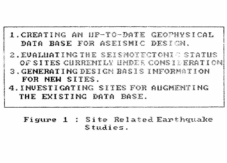
I -p.

M SiJ^iS

FOS NEW SITES4 . INUESTIGfiTINCi

THE EXISTI

i f I i s*r

J-d JL Hil I ''iJlJ'M

LI'S? Ji- ' - ,Sl '§ a

"W ;*••»• s r 5

l ^ A 5

JL f". Ms. S

1 gure i te He 1 -at ud ies ,

VI

J : (!•

(T i '•/•

rf! irj pit, ,'s i W ^

jm \ i

* is*

h O c(I

f

. , j y 5 j-885^ Afeiij |i»-te x / ^tn4

* B f f i

' • • " . - - " ' • • ' , ,

nap

rT"f ;

F. M s * <

W

-""' I

!

' HS'ffia

3 V

En

vat

I

3.DXSFLftCEi

4.RUPTURE PROPAGAXI

5.ELASTIC CONTENTS OF TOF WAUE PROPAGATION.

6.INTENSITY8.SEISHIC

9.STRESS DROP.18.LOCAL TRANSFER FUNCTIO

JU-JU =a- a

»:*-.• ra

J. JL A.

3: Information fPOP Data Ease

2,A REfe AU AILABLE FOR ST RAINACCUMULATION.

USHEAE RESISTANCE ALONG THE FAULT4.AMOUNT OF SUDDEN DISPLACEMENT.5,SIZE OF THE MOST RECENT EUENT.£ TIME! ELAPSED SINCE THE LAST

STRONG EARTHQUAKE.' : .LOCAL GROUND Of ARA CTERIS TICS.;;,TVF!i OF STRUCTURES.

4: SeisMic Risk Factors

_FEA j^J^T^ _RECOGN I 2E FA LJ LT CA PA BILI 1 V1.Fault Scares.2.Rift Ualleys.3. Over- steepened ba.se of Mountain fronts4. Faceted or- t^iangula^ spurs or1 ri5 . S hu tt'?r x1 i cl^e s .6. Off set str-9AMS,? . I > r v A i n a g e l i r i e S j g u t l i e s o r8.Benches.9.Sags or sacr ponds.

10.Closed depress ions, troughs11.Side h i l l r i d g e s .i2.TerrAces along s ides of h i l l s . j13 .Saddles .14.Mole t r a c k s .15 . Ope n F i s s uan-e s .16.Notches of unusual orientation

ox* position relative to strati-graphy or lithologicaldifferences jin resistance to erosion.

17.Terraces upstream froK scarps.18.Furrows.19.Ground waier Carriers hacked fey

spring alignwientj vegetationalcontrast or lineaments.

28. Folding OP warping of young alluvial for erosional surfaces with sediwen-jtation or erosion. !

Figure 5 : Recognition of Active Faults

(Aides for Field Checks)

60.0100.0i.0-0

30.0

200

700 80 0 90.0

laure 6 : Tea degree Squares corresponding to the region numbers ofTable II used for presenting the Earthquake MagnitudeFrequency Data for the Indian subcontinent. (Boundaries ofthe map are based on digitized data obtained from the Auto-matic Cartography Cell of Survey of India.)

ow I °° TYPE I

oLU ° o oO 0 0 0 0 0 0 0 0 0 0 ° ° O Q O O O O O O

LU IS •"> ° TYPE II

O ft o ° ° o o,,, „ ° ° o om O O O O O O 0 ° ° Q O O Q Ok

O . ° O O O ° o o T Y P E I I Io o

QJ 1 0 0 0 0 0 ° Q O ° O O 0 O O O O O

TIME

Figure 7 ; TYPE I,II AND III PATTERNS OF EARTHQUAKE OCCURRENCE.

[The ordinate represents the number of shocks per day inthe area under observation against, absolute time. The x3ign marks the time of occurrence of the main shock inType I and II patterns. In typo III patterns bhe main3hock cannot be identified with '^rtainty.J

'*(

*t %

i

n

••rp

flj

0 ft

rt ni rti 3

awBiffl? j » 5 , »!•«, jKSSj

!Hftr lts• W ^llr

i ' g wins i I

Is!

ft

0 fl

WSils. aSS!E

JWIS

•H

1/f

0

m

s

X

o! u

o

S3DO1

3

0•H

0

co

(3

(0i-H

oo

0)in3

-P

IB

X

^...^Bi^ia^...,.,

Tl T2 T3 T4 T5 TN-I TN

HARMONIC OSCILLATORS OF DIFERENTNATURAL FREQUENCIES

> WVNAW

P(t)

m-»Lumped mass kxk -» Spring constant mxc-*Damping ex

cx+kx = P (t )

P(t)

UJ

2= a.< LU

2 cr

= C1

PERIOD

Figure 9 : RESPONSE SPECTRUM - AN ILLUSTRATION

(A time dependent force P(t) is applied separately toSingle Degree of Freedom systems of natural periodTl,T2,T3,...TN. The maximum response of each systemplotted against the natural period is the responsespectrum of P(t).)

oo_JLU ^> LULU

O(I)

LU OCC —I

OQ3LU

VELOCITY

AMPLIFICATION

FACTOR

Sv

PERIOD (LOG SCALE)

Figure 10 : PEAK GROUND MOTION PARAMETERS AND RESPONSE SPECTRA.

[At high frequencies the spectral acceleration approachesthe peak ground acceleration; at low frequencies the spectraldisplacement approaches the ground displacement]

Published by Library & Information Services, BARC, Bombay 400 085, India.