Embed Size (px)
Citation preview

Chapter 4
Basic category theory
“...We know only a very few—and, therefore, very precious—schemes whose unifyingpowers cross many realms.” – Marvin Minsky.1
Categories, or an equivalent notion, have already been secretly introduced as ologs.One can think of a category as a graph (as in Section 3.3) in which certain paths havebeen declared equivalent. (Ologs demand an extra requirement that everything in sightbe readable in natural language, and this cannot be part of the mathematical definitionof category.) The formal definition of category is given in Definition 4.1.1.1, but itwill not be obviously the same as the “graph+path equivalences” notion; the latter wasgiven in Definition 3.5.2.6 as the definition of a schema. Once we talk about how differentcategories can be compared using functors (Definition 4.1.2.1), and how different schemascan be compared using schema mappings (Definition 4.4.1.2), we will prove that the twonotions are equivalent (Theorem 4.4.2.3).
4.1 Categories and FunctorsIn this section we give the standard definition of categories and functors. These, togetherwith natural transformations (Section 4.3), form the backbone of category theory. Wealso give some examples.
4.1.1 CategoriesIn everyday speech we think of a category as a kind of thing. A category consists of acollection of things, all of which are related in some way. In mathematics, a categorycan also be construed as a collection of things and a type of relationship between pairsof such things. For this kind of thing-relationship duo to count as a category, we need tocheck two rules, which have the following flavor: every thing must be related to itself bysimply being itself, and if one thing is related to another and the second is related to athird, then the first is related to the third. In a category, the “things” are called objectsand the “relationships” are called morphisms.
In various places throughout this book so far we have discussed things of varioussorts, e.g. sets, monoids, graphs. In each case we discussed how such things should be
1[Min, Problems of disunity, p. 126].
113

114 CHAPTER 4. BASIC CATEGORY THEORY
appropriately compared. In each case the “things” will stand as the objects and the“appropriate comparisons” will stand as the morphisms in the category. Here is thedefinition.Definition 4.1.1.1. A category C is defined as follows: One announces some constituents(A. objects, B. morphisms, C. identities, D. compositions) and asserts that they conformto some laws (1. identity law, 2. associativity law). Specifically, one announces:
A. a collection ObpCq, elements of which are called objects;
B. for every pair x, y P ObpCq, a set HomCpx, yq P Set. It is called the hom-setfrom x to y; its elements are called morphisms from x to y; 2
C. for every object x P ObpCq, a specified morphism denoted idx P HomCpx, xqcalled the identity morphism on x; and
D. for every three objects x, y, z P ObpCq, a function
˝ : HomCpy, zq ˆHomCpx, yq Ñ HomCpx, zq,
called the composition formula.Given objects x, y P ObpCq, we can denote a morphism f P HomCpx, yq by f : xÑ y; wesay that x is the domain of f and that y is the codomain of f . Given also g : y Ñ z,the composition formula is written using infix notation, so g ˝ f : xÑ z means ˝pg, fq PHomCpx, zq.
One asserts that the following law holds:1. for every x, y P ObpCq and every morphism f : xÑ y, we have
f ˝ idx “ f and idy ˝ f “ f ;
and;
2. if w, x, y, z P ObpCq are any objects and f : w Ñ x, g : x Ñ y, and h : y Ñ zare any morphisms, then the two ways to compose are the same:
ph ˝ gq ˝ f “ h ˝ pg ˝ fq P HomCpw, zq.
Remark 4.1.1.2. There is perhaps much that is unfamiliar about Definition 4.1.1.1 butthere is also one thing that is strange about it. The objects ObpCq of C are said tobe a “collection” rather than a set. This is because we sometimes want to talk aboutthe category of all sets, in which every possible set is an objects, and if we try to saythat the collection of sets is itself, we run into Russell’s paradox. Modeling this wasa sticking point in the foundations of category theory, but it was eventually fixed byGrothendieck’s notion of expanding universes. Roughly the idea is to choose some hugeset κ (with certain properties making it a universe), to work entirely inside of it whenpossible, and to call anything in that world κ-small (or just small if κ is clear fromcontext). When we need to look at κ itself, we choose an even bigger universe κ1 andwork entirely within it.
A category in which the collection ObpCq is a set (or in the above language, a smallset) is called a small category. From here on out we will not take care of the difference,referring to ObpCq as a set. We do not think this will do any harm to scientists usingcategory theory, at least not in the beginning phases of their learning.
2The reason for the notation Hom and the word hom-set is that morphisms are often called homo-morphisms, e.g. in group theory.

4.1. CATEGORIES AND FUNCTORS 115
Example 4.1.1.3 (The category Set of sets). Chapter 2 was all about the category of sets,denoted Set. The objects are the sets and the morphisms are the functions; we evenused the current notation, referring to the set of functions X Ñ Y as HomSetpX,Y q.The composition formula ˝ is given by function composition, and for every set X, theidentity function idX : X Ñ X serves as the identity morphism for X P ObpSetq. Thetwo laws clearly hold, so Set is indeed a category.Example 4.1.1.4 (The category Fin of finite sets). Inside the category Set is a subcategoryFin Ď Set, called the category of finite sets. Whereas an object S P ObpSetq is a setthat can have arbitrary cardinality, we define Fin such that its objects include all (andonly) the sets S with finitely many elements, i.e. |S| “ n for some natural number n P N.Every object of Fin is an object of Set, but not vice versa.
Although Fin and Set have a different collection of objects, their morphisms are insome sense “the same”. For any two finite sets S, S1 P ObpFinq, we can also think ofS, S1 P ObpSetq, and we have
HomFinpS, S1q “ HomSetpS, S
1q.
That is a morphism in Fin between finite sets S and S1 is simply a function f : S Ñ S1.Example 4.1.1.5 (The category Mon of monoids). We defined monoids in Definition3.1.1.1 and monoid homomorphisms in Definition 3.1.4.1. Every monoidM :“ pM, e, ‹M qhas an identity homomorphism idM : MÑM, given by the identity function idM : M Ñ
M . To compose two monoid homomorphisms f : MÑM1 and g : M1 ÑM2, we com-pose their underlying functions f : M ÑM 1 and g : M 1 ÑM2, and check that the resultg ˝ f is a monoid homomorphism. Indeed,
g ˝ fpeq “ gpe1q “ e2
g ˝ fpm1 ‹M m2q “ gpfpm1q ‹M 1 fpm2qq “ g ˝ fpm1q ‹M2 g ˝ fpm2q.
It is clear that the two laws hold, so Mon is a category.Exercise 4.1.1.6 (The category Grp of groups). Suppose we set out to define a categoryGrp, having groups as objects and group homomorphisms as morphisms, see Definition3.2.1.16. Show (to the level of detail of Example 4.1.1.5) that the rest of the conditionsfor Grp to be a category are satisfied. ♦
Exercise 4.1.1.7 (The category PrO of preorders). Suppose we set out to define a cate-gory PrO, having preorders as objects and preorder homomorphisms as morphisms (seeDefinition 3.4.4.1). Show (to the level of detail of Example 4.1.1.5 that the rest of theconditions for PrO to be a category are satisfied. ♦
Example 4.1.1.8 (Non-category 1). So what’s not a category? Two things can go wrong:either one fails to specify all the relevant constituents (A, B, C, D from Definition 4.1.1.1,or the constituents do not obey the laws (1, 2).
Let G be the following graph,
G “ a‚
f // b‚g // c‚ .
Suppose we try to define a category G by faithfully recording vertices as objects andarrows as morphisms. Will that be a category?

116 CHAPTER 4. BASIC CATEGORY THEORY
Following that scheme, we put ObpGq “ ta, b, cu. For all 9 pairs of objects we need ahom-set. Say
HomGpa, aq “ H HomGpa, bq “ tfu HomGpa, cq “ HHomGpb, aq “ H HomGpb, bq “ H HomGpb, cq “ tguHomGpc, aq “ H HomGpc, bq “ H HomGpc, cq “ H
If we say we are done, the listener should object that we have given neither identitiesnor a composition formula. In fact, it is impossible to give identities under our scheme,because e.g. HomGpa, aq “ H.
Suppose we fix that problem, adding an element to each of our “diagonals” so that
HomGpa, aq “ tidau, HomGpb, bq “ tidbu, and HomGpc, cq “ tidcu.
What about a composition formula? We need a function HomGpa, bq ˆ HomGpb, cq ÑHomGpa, cq, but the domain is nonempty and the codomain is empty; there is no suchfunction.
Again, we must make a change, adding an element to make
HomGpa, cq “ thu.
We would now say g ˝ f “ h. Finally, this does the trick and we have a category. Acomputer could check this quickly, as can someone with good intuition for categories;for everyone else, it may be a painstaking process involving determining whether thereis a unique composition formula for each of the 27 pairs of hom-sets and whether theassociative law holds in the 81 necessary cases. Luckily this computation is “sparse”(lots of H’s), so it’s not as bad as it first seems.
Redrawing all the morphisms as arrows, our graph has become:
G “ a‚ida ::
f //
h
88b‚
idb
�� g // c‚ idcdd
Example 4.1.1.9 (Non-category 2). In this example, we will make a faux-category F withone object and many morphisms. The problem here will be our composition formula.
Define F to have one object ObpFq “ t,u, and HomF p,,,q “ N. Define id, “ 1 PN. Define the composition formula ˝ : N ˆ N Ñ N by m ˝ n “ mn. This is a perfectlycromulent function, but it does not work right as a composition formula. Indeed, for theidentity law to hold, we would need m1 “ m “ 1m, and one side of this is false. For theassociativity law to hold, we would need pmnqp “ mpn
pq, but this is also not the case.
To fix this problem we have to completely revamp our composition formula. It wouldwork to use multiplication, m ˝ n “ m ˚ n. Then the identity law would read 1 ˚m “
m “ m˚1, and that holds; and the associativity law would read pm˚nq ˚p “ m˚ pn˚pq,and that holds.Example 4.1.1.10 (The category of preorders with joins). Suppose that we are onlyinterested in preorders pX,ďq for which every pair of elements has a join. We saw inExercise 3.4.2.3 that not all preorders have this property. However we can create acategory C in which every object does have this property. To begin we put ObpCq “tpX,ďq P ObpPrOq | pX,ďq has all joinsu. But what about morphisms?

4.1. CATEGORIES AND FUNCTORS 117
One option would be to put in no morphisms (other than identities), and to justconsider this collection of objects as having no structure other than a set.
Another option would be to put in exactly the same morphisms as in PrO: for anyobjects a, b P ObpCq we consider a and b as regular old preorders, and put HomCpa, bq :“HomPrOpa, bq. The resulting category of preorders with joins is called the full subcategoryof PrO spanned by the preorders with joins.3
A third option, and the one perhaps that would jump out to a category theorist, isto take the choice about how we define our objects as a clue to how we should defineour morphisms. Namely, if we are so interested in joins, perhaps we want joins to bepreserved under morphisms. That is, if f : pX,ďXq Ñ pY,ďY q is a morphism of preordersthen for any join w “ x_ x1 in X we might want to enforce that fpwq “ fpxq _ fpx1q inY . Thus a third possibility for the morphisms of C would be
HomCpa, bq :“ tf P HomPrOpa, bq | f preserves joinsu.
One can check easily that the identity morphisms preserve joins and that compositions ofjoin-preserving morphisms are join-preserving, so this version of homomorphisms makesfor a well-defined category.Example 4.1.1.11 (Category FLin of finite linear orders). We have a category PrO ofpreorders, and some of its objects are finite (nonempty) linear orders. Let FLin bethe full subcategory of PrO spanned by the linear orders. That is, following Definition3.4.4.1, given linear orders X,Y , every morphism of preorders X Ñ Y counts as amorphism in FLin:
HomFLinpX,Y q “ HomPrOpX,Y q.
Exercise 4.1.1.12. Let FLin be the category of finite linear orders, defined in Example4.1.1.11. For n P N, let rns be the linear order defined in Example 3.4.1.7. What are thecardinalities of the following sets:
a.) HomFLinpr0s, r3sq;
b.) HomFLinpr3s, r0sq;
c.) HomFLinpr2s, r3sq;
d.) HomFLinpr1s, rnsq?
e.) (Challenge) HomFLinprms, rnsq?
It turns out that the category FLin of linear orders is sufficiently rich that much of al-gebraic topology (the study of arbitrary spaces, such as Mobius strips and 7-dimensionalspheres) can be understood in its terms. See Example 4.6.1.6. ♦
Example 4.1.1.13 (Category of graphs). We defined graphs in Definition 3.3.1.1 andgraph homomorphisms in Definition 3.3.3.1. To see that these are sufficient to form acategory is considered routine to a seasoned category-theorist, so let’s see why.
Since a morphism from G “ pV,A, src, tgtq to G1 “ pV 1, A1, src1, tgt1q involves twofunctions f0 : V Ñ V 1 and f1 : A Ñ A1, the identity and composition formulas willsimply arise from the identity and composition formulas for sets. Associativity willfollow similarly. The only thing that needs to be checked, really, is that the compositionof two such things, each satisfying (3.6), will itself satisfy (3.6). Just for completeness,we check that now.
3The definition of full subcategories will be given as Definition 4.6.3.1.

118 CHAPTER 4. BASIC CATEGORY THEORY
Suppose that f “ pf0, f1q : G Ñ G1 and g “ pg0, g1q : G1 Ñ G2 are graph homomor-phisms, where G2 “ pV 2, A2, src2, tgt2q. Then in each diagram below
Af1 //
src
��
A1g1 //
src1
��
A2
src2
��V
f0
// V 1g0// V 2
Af1 //
tgt
��
A1
tgt1
��
g1 // A2
tgt2
��V
f0
// V 1g0// V 2
(4.1)
the left-hand square commutes because f is a graph homomorphism and the right-handsquare commutes because g is a graph homomorphism. Thus the whole rectangle com-mutes, meaning that g ˝ f is a graph homomorphism, as desired.
We denote the category of graphs and graph homomorphisms by Grph.Remark 4.1.1.14. When one is struggling to understand basic definitions, notation, andstyle, a phase which naturally occurs when learning new mathematics (or any new lan-guage), the above example will probably appear long and tiring. I’d say you’ve masteredthe basics when the above example really does feel straightforward. Around this time,I imagine you’ll begin to get a sense of the remarkable organisational potential of thecategorical way of thinking.Exercise 4.1.1.15. Let F be a vector field on R2. Recall that for two points x, x1 P R2,any curve C with endpoints x and x1, and any parameterization r : ra, bs Ñ C, the lineintegral
ş
CF prq¨dr returns a real number. It does not depend on r, except its orientation
(direction). Therefore, if we think of C has having an orientation, say going from x tox1, then
ş
CF is a well-defined real number. If C goes from x to x1, let’s suggestively
write C : xÑ x1. Define an equivalence relation „ on the set of oriented curves in R2 bysaying C „ C 1 if
• C and C 1 start at the same point,
• C and C 1 end at the same point, and
•ş
CF “
ş
C1F .
Suppose we try to make a category CF as follows. Put ObpCF q “ R2, and for everypair of points x, x1 P R2, let HomCF
px, x1q “ tC : x Ñ x1u{ „, where C : x Ñ x1 is anoriented curve and „ means “same line integral”, as explained above.
Is there an identity morphism and a composition formula that will make CF into acategory? ♦
4.1.1.16 Isomorphisms
In any category we have a notion of isomorphism between objects.
Definition 4.1.1.17. Let C be a category and let X,Y P ObpCq be objects. An isomor-phism f from X to Y is a morphism f : X Ñ Y in C, such that there exists a morphismg : Y Ñ X in C such that
g ˝ f “ idX and f ˝ g “ idY .
In this case we say that the morphism f is invertible and that g is the inverse of f . Wemay also say that the objects X and Y are isomorphic.

4.1. CATEGORIES AND FUNCTORS 119
Example 4.1.1.18. If C “ Set is the category of sets, then the above definition coincidesprecisely with the one given in Definition 2.1.2.8.
Exercise 4.1.1.19. Suppose that G “ pV,A, src, tgtq and G1 “ pV 1, A1, src1, tgt1q aregraphs and that f “ pf0, f1q : G Ñ G1 is a graph homomorphism (as in Definition3.3.3.1).
a.) If f is an isomorphism in Grph, does this imply that f0 : V Ñ V 1 and f1 : A Ñ A1
are isomorphisms in Set?
b.) If so, why; and if not, show a counterexample (where f is an isomorphism but eitherf0 or f1 is not).
♦
Exercise 4.1.1.20. Suppose that G “ pV,A, src, tgtq and G1 “ pV 1, A1, src1, tgt1q aregraphs and that f “ pf0, f1q : G Ñ G1 is a graph homomorphism (as in Definition3.3.3.1).
a.) If f0 : V Ñ V 1 and f1 : A Ñ A1 are isomorphisms in Set, does this imply that f isan isomorphism in Grph?
b.) If so, why; and if not, show a counterexample (where f0 and f1 are isomorphismsbut f is not).
♦
Lemma 4.1.1.21. Let C be a category and let „ be the relation on ObpCq given by sayingX „ Y iff X and Y are isomorphic. Then „ is an equivalence relation.
Proof. The proof of Lemma 2.1.2.12 can be mimicked in this more general setting.�
4.1.1.22 Another viewpoint on categories
Here is an alternate definition of category, using the work we did in Chapter 2.
Exercise 4.1.1.23. Suppose we begin our definition of category as follows.A category, C consists of a sequence pObpCq,HomC , dom, cod, ids, ˝q, where
1. ObpCq is a set,4
2. HomC is a set, and dom, cod : HomC Ñ ObpCq are functions,
3. ids : ObpCq Ñ HomC is a function, and
4See Remark 4.1.1.2.

120 CHAPTER 4. BASIC CATEGORY THEORY
4. ˝ is a function as depicted in the commutative diagram below
HomC cod
))
dom
""
HomC ˆObpCq HomC
X
X
˝
hh
//
��
yHomC
cod//
dom
��
ObpCq
HomCcod
//
dom
��
ObpCq
ObpCq
(4.2)
a.) Express the fact that for any x P ObpCq the morphism idx points from x to x interms of the functions id, dom, cod.
b.) Express the condition that composing a morphism f with an appropriate identitymorphism yields f .
c.) Express the associativity law in these terms (Hint: Proposition 2.5.1.17 may beuseful).
♦
Example 4.1.1.24 (Partial olog for a category). Below is an olog that captures some ofthe essential structures of a category.
a morphismin C
has as codomain
))
has as domain
��
a pair pg, fqof composablemorphisms
X
Xhas as composition
dd
yieldsas g //
yields as f
��
y
a morphismin C has as
codomain
//
has as domain
��
an object of C
a morphismin C has as
codomain
//
has as domain
��
an object of C
an object of C
(4.3)
Missing from (4.3) is the notion of identity morphism (as an arrow from pan objectof Cq to pa morphism in Cq) and the associated path equivalences, as well as the identity

4.1. CATEGORIES AND FUNCTORS 121
and associativity laws. All of these can be added to the olog, at the expense of someclutter.Remark 4.1.1.25. Perhaps it is already clear that category theory is very interconnected.It may feel like everything relates to everything, and this feeling may intensify as yougo on. However, the relationships between different notions are rigorously defined, andnot random. Moreover, almost everything presented in this book can be formalized ina proof system like Coq (the most obvious exceptions being things like the readabilityrequirement of ologs and the modeling of scientific applications).
Whenever you feel cognitive vertigo, look to formal definitions as the ground of yourunderstanding. It is good practice to make sure that the intuition you’ve developedactually “touches down” on that ground, i.e. that your way of thinking can be built upsolidly from the foundational definitions.
4.1.2 FunctorsA category C “ pObpCq,HomC , dom, cod, ids, ˝q, involves a set of objects, a set of mor-phisms, a notion of domains and codomains, a notion of identity morphisms, and acomposition formula. For two categories to be comparable, these various componentsshould be appropriately comparable.
Definition 4.1.2.1. Let C and C1 be categories. A functor F from C to C1, denotedF : C Ñ C1, is defined as follows: One announces some constituents (A. on-objects part,B. on-morphisms part) and asserts that they conform to some laws (1. preservation ofidentities, 2. preservation of composition). Specifically, one announces
A. a function ObpF q : ObpCq Ñ ObpC1q, which we sometimes denote simply byF : ObpCq Ñ ObpC1q; and
B. for every pair of objects c, d P ObpCq, a function
HomF pc, dq : HomCpc, dq Ñ HomC1pF pcq, F pdqq,
which we sometimes denote simply by F : HomCpc, dq Ñ HomC1pF pcq, F pdqq.
One asserts that the following laws hold:
1. Identities are preserved by F . That is, for any object c P ObpCq, we haveF pidcq “ idF pcq; and
2. Composition is preserved by F . That is, for any objects b, c, d P ObpCq andmorphisms g : bÑ c and h : cÑ d, we have F ph ˝ gq “ F phq ˝ F pgq.
Example 4.1.2.2 (Monoids have underlying sets). Recall from Definition 3.1.1.1 that ifM “ pM, e, ‹q is a monoid, then M is a set. And recall from Definition 3.1.4.1 that iff : MÑM1 is a monoid homomorphism then f : M ÑM 1 is a function. Thus we havea functor
U : Mon Ñ Set
that takes every monoid to its underlying set and every monoid homomorphism to itsunderlying function.
Given two monoids M “ pM, e, ‹q and M1 “ pM 1, e1, ‹1q, there may be many func-tions from M to M 1 that do not arise from monoid homomorphisms. It is often useful tospeak of such functions. For example, one could assign to every command in one video

122 CHAPTER 4. BASIC CATEGORY THEORY
game V a command in another video game V 1, but this may not work in the “monoidyway” when performing a sequence of commands. By being able to speak of M as a set,or as M as a monoid, and understanding the relationship U between them, we can beclear about where we stand at all times in our discussion.Example 4.1.2.3 (Groups have underlying monoids). Recall that a group is just a monoidpM, e, ‹q with the extra property that every element m PM has an inverse m1 ‹m “ e “m ‹m1. Thus to every group we can assign its underlying monoid. Similarly, a grouphomomorphism is just a monoid homomorphism of its underlying monoids. This meansthat there is a functor
U : Grp Ñ Mon
that sends every group or group homomorphism to its underlying monoid or monoidhomomorphism. That identity and composition are preserved is obvious.
Slogan 4.1.2.4.
“ Out of all our available actions, some are reversable. ”
Application 4.1.2.5. Suppose you’re a scientist working with symmetries. But then sup-pose that the symmetry breaks somewhere, or you add some extra observable which isnot reversible under the symmetry. You want to seamlessly relax the requirement thatevery action be reversible without changing anything else. You want to know where youcan go, or what’s allowed. The answer is to simply pass from the category of groups (orgroup actions) to the category of monoids (or monoid actions).
We can also reverse this change of perspective. Recall that in Example 3.1.2.9 wediscussed a monoid M controlling the actions of a video game character. The characterposition (P ) could be moved up (u), moved down (d), or moved right (r). The pathequivalences P.u.d “ P and P.d.u “ P imply that these two actions are mutuallyinverse, whereas moving right has no inverse. This, plus equivalences P.r.u “ P.u.rand P.r.d “ P.d.r, defined a monoid M .
Inside M is a submonoid G, which includes just upward and downward movement.It has one object, just like M , i.e. ObpMq “ tP u “ ObpGq. But it has fewer morphisms.In fact there is a monoid isomorphism G – Z because we can assign to any movement inG the number of ups, e.g. P.u.u.u.u.u is assigned the integer 5, P.d.d.d is assigned theinteger ´3, and P.d.u.u.d.d.u is assigned the integer 0 P Z. But Z is a group, becauseevery integer has an inverse.
Thus we can consider G as a group G1 P ObpGrpq or as a monoid G2 P ObpMonq.It is better to consider G as a group, because groups are more structured than monoids.It’s as though putting G in Grp gives it more “potential energy” than putting it in Mon— we can always “drop it down” from Grp to Mon, but not vice versa. The way tomake this precise is that we can make use of the functor U : Grp Ñ Mon from Example4.1.2.3 and find that UpG1q “ G2. But to find a functor F : Mon Ñ Grp such thatF pG2q “ G1 would be much more ad hoc.
The upshot is that we can use functors to compare groups and monoids.♦♦
Example 4.1.2.6. Recall that we have a category Set of sets and a category Fin offinite sets. We said that Fin was a subcategory of Set. In fact we can think of this“subcategory” relationship in terms of functors, just like we thought of the “subset”relationship in terms of functions in Example 2.1.2.3. That is, if we have a subset

4.1. CATEGORIES AND FUNCTORS 123
S Ď S1, then every element s P S is an element of S1, so we make a function f : S Ñ S1
such that fpsq “ s P S1.To give a functor i : Fin Ñ Set, we have to announce how it will work on objects
and how it will work on morphisms. We begin by announcing a function i : ObpFinq ÑObpSetq. But that’s easy because ObpFinq Ď ObpSetq, so we proceed as above: ipSq “ Sfor any S P ObpFinq. We also have announce, for each pair of objects S, S1 P ObpFinq,a function
i : HomFinpS, S1q Ñ HomSetpS, S
1q.
But again, that’s easy because we know by definition (see Example 4.1.1.4) that thesetwo sets are equal, HomFinpS, S
1q “ HomSetpS, S1q. Hence we can simply take i to be
the identity function on morphisms. It is easy to see that identites and compositions arepreserved by i. Therefore, we have defined a functor i.Exercise 4.1.2.7 (Forgetful functors between types of orders). A partial order is just apreorder with a special property. A linear order is just a partial order with a specialproperty.
a.) Is there an “obvious” functor FLin Ñ PrO?
b.) Is there an “obvious” functor PrO Ñ FLin?
♦
Proposition 4.1.2.8 (Preorders to graphs). Let PrO be the category of preorders andGrph be the category of graphs. There is a functor P : PrO Ñ Grph such that for anypreorder X “ pX,ďq, the graph P pX q has vertices X.
Proof. Given a preorder X “ pX,ďXq, we can make a graph F pX q with vertices Xand an arrow x Ñ x1 whenever x ďX x1, as in Remark 3.4.1.10. More precisely, thepreorder ďX is a relation, i.e. a subset RX Ď X ˆX, which we think of as a functioni : RX Ñ X ˆX. Composing with projections π1, π2 : X ˆX Ñ X gives us
srcX :“ π1 ˝ i : RX Ñ X and tgtX :“ π2 ˝ i : RX Ñ X.
Then we put F pX q :“ pX,RX , srcX , tgtX q. This gives us a function F : ObpPrOq ÑObpGrphq.
Suppose now that f : X Ñ Y is a preorder morphism (where Y “ pY,ďY q). This is afunction f : X Ñ Y such that for any px, x1q P XˆX, if x ďX x1 then fpxq ď fpx1q. Butthat’s the same as saying that there exists a dotted arrow making the following diagramof sets commute
RX //
��
X ˆX
fˆf
��RY // Y ˆ Y
(Note that there cannot be two different dotted arrows making that diagram commutebecause RY Ñ Y ˆ Y is a monomorphism.) Our commutative square is precisely what’sneeded for a graph homomorphism, as shown in Exercise 3.3.3.7. Thus, we have definedF on objects and on morphisms. It is clear that F preserves identity and composition.
�
Exercise 4.1.2.9. In Proposition 4.1.2.8 we gave a functor P : PrO Ñ Grph.
124 CHAPTER 4. BASIC CATEGORY THEORY
a.) Is every graph G P ObpGrphq in the image of P (or more precisely, is the function
ObpP q : ObpPrOq Ñ ObpGrphq
surjective)?
b.) If so, why; if not, name a graph not in the image.
c.) Suppose that G,H P ObpGrphq are two graphs that are in the image of P . Is everygraph homomorphism f : GÑ H in the image of HomP ? In other words, does everygraph homomorphism between G and H come from a preorder homomorphism?
♦
Remark 4.1.2.10. There is a functor W : PrO Ñ Set sending pX,ďq to X. Thereis a functor T : Grph Ñ Set sending pV,A, src, tgtq to V . When we understand thecategory of categories (Section 4.1.2.27), it will be clear that Proposition 4.1.2.8 can besummarized as a commutative triangle in Cat,
PrO P //
W
��
Grph
T
��Set
Exercise 4.1.2.11 (Graphs to preorders). Recall from (2.3) that every function f : A ÑB has an image, imf pAq Ď B. Use this idea and Example 3.4.1.16 to construct afunctor Im : Grph Ñ PrO such that for any graph G “ pV,A, src, tgtq, the preorderhas elements given by the vertices of G (i.e. we have ImpGq “ pV,ďGq, for some orderingďG). ♦
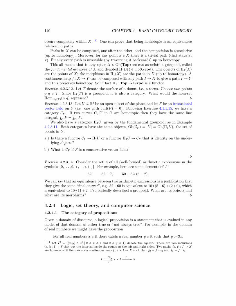
Exercise 4.1.2.12. What is the preorder ImpGq when G P ObpGrphq is the followinggraph?
G :“
v‚
f // w‚
h
??
g
x‚
y‚
i �� j
z‚
k
__
♦
Exercise 4.1.2.13. Consider the functor Im : Grph Ñ PrO constructed in Exercise4.1.2.11.
a.) Is every preorder X P ObpPrOq in the image of Im (or more precisely in the imageof ObpImq : ObpGrphq Ñ ObpPrOq)?
b.) If so, why; if not, name a preorder not in the image.
c.) Suppose that X ,Y P ObpPrOq are two preorders that are in the image of Im. Isevery preorder morphism f : X Ñ Y in the image of HomIm? In other words, doesevery preorder homomorphism between X and Y come from a graph homomorphism?

4.1. CATEGORIES AND FUNCTORS 125
♦
Exercise 4.1.2.14. We have functors P : PrO Ñ Grph and Im : Grph Ñ PrO.
a.) What can you say about Im ˝ P : PrO Ñ PrO?
b.) What can you say about P ˝ Im : Grph Ñ Grph?
♦
Exercise 4.1.2.15. Consider the functors P : PrO Ñ Grph and Im : Grph Ñ PrO.And consider the chain graph rns of length n from Example 3.3.1.8 and the linear orderrns of length n from Example 3.4.1.7. To differentiate the two, let’s rename them forthis exercise as rnsGrph P ObpGrphq and rnsPrO P ObpPrOq. We see a similaritybetween rnsGrph and rnsPrO, and we might hope that our functors help us formalize thissimilarity. That is, we might hope that one of the following hold:
P prnsPrOq –? rnsGrph or ImprnsGrphq –
? rnsPrO.
Do either, both, or neither of these hold? ♦
Remark 4.1.2.16. In the course announcement for 18-S996, I wrote the following:
It is often useful to focus ones study by viewing an individual thing, or agroup of things, as though it exists in isolation. However, the ability torigorously change our point of view, seeing our object of study in a differentcontext, often yields unexpected insights. Moreover this ability to changeperspective is indispensable for effectively communicating with and learningfrom others. It is the relationships between things, rather than the thingsin and by themselves, that are responsible for generating the rich varietyof phenomena we observe in the physical, informational, and mathematicalworlds.
This holds at many different levels. For example, one can study a group (in the sense ofDefinition 3.2.1.1) in isolation, trying to understand its subgroups or its automorphisms,and this is mathematically interesting. But one can also view it as a quotient of somethingelse, or as a subgroup of something else. One can view the group as a monoid and lookat monoid homomorphisms to or from it. One can look at the group in the context ofsymmetries by seeing how it acts on sets. These changes of viewpoint are all clearlyand formally expressible within category theory. We know how the different changes ofviewpoint compose and how they fit together in a larger context.Exercise 4.1.2.17.
a.) Is the above quote also true in your scientific discipline of expertise? How so?
b.) Can you imagine a way that category theory can help catalogue the kinds of rela-tionships or changes of viewpoint that exist in your discipline?
c.) What kinds of structures that you use often really deserve to be better formalized?
Keep this kind of question in mind for your final project. ♦
Example 4.1.2.18 (Free monoids). Let G be a set. We saw in 3.1.1.15 that ListpGq is amonoid, called the free monoid on G. Given a function f : GÑ G1, there is an inducedfunction Listpfq : ListpGq Ñ ListpG1q, and this preserves the identity element r s andconcatenation of lists, so Listpfq is a monoid homomorphism. It is easy to check thatList : Set Ñ Mon is a functor.

126 CHAPTER 4. BASIC CATEGORY THEORY
Application 4.1.2.19. In Application 2.1.2.10 we discussed an isomorphism NucDNA –
NucRNA given by RNA transcription. Applying the functor List we get a function
ListpNucDNAq–ÝÑ ListpNucRNAq,
which will send sequences of DNA nucleotides to sequences of RNA nucleotides and viceversa. This is performed by polymerases.
♦♦
Exercise 4.1.2.20. Let G “ t1, 2, 3, 4, 5u, G1 “ ta, b, cu, and let f : G Ñ G1 be given bythe sequence pa, c, b, a, cq.5 Then if L “ r1, 1, 3, 5, 4, 5, 3, 2, 4, 1s, what is ListpfqpLq? ♦
Exercise 4.1.2.21. We can rephrase our notion of functor in terms compatible with Ex-ercise 4.1.1.23. We would begin by saying that a functor F : C Ñ C1 consists of twofunctions,
ObpF q : ObpCq Ñ ObpC1q and HomF : HomC Ñ HomC1 ,
which we call the on-objects part and the on-morphisms part, respectively. They mustfollow some rules, expressed by the commutativity of the following squares in Set:
HomCdom //
HomF
��
ObpCq
ObpF q��
HomC1dom// ObpC1q
HomCcod //
HomF
��
ObpCq
ObpF q��
HomC1cod// ObpC1q
(4.4)
ObpCq
ObpF q��
id // HomC
HomF
��ObpC1q
id// HomC1
HomC ˆObpCq HomC˝ //
��
HomC
HomF
��HomC1 ˆObpC1q HomC1 ˝
// HomC1
(4.5)
Where does the (unlabeled) left-hand function in the bottom right diagram come from?Hint: use Exercise 2.5.1.19.
Consider Diagram (4.2) and imagine it as though contained in a pane of glass. Thenimagine a parallel pane of glass involving C1 in place of C everywhere.
a.) Draw arrows from the C pane to the C1 pane, each labeled ObpF q or HomF as seemsappropriate.
b.) If F is a functor (i.e. satisfies (4.4) and (4.5)), do all the squares in your drawingcommute?
c.) Does the definition of functor involve anything not captured in this setup?
♦
Example 4.1.2.22 (Paths-graph). Let G “ pV,A, src, tgtq be a graph. Then for any pair ofvertices v, w P G, there is a set PathGpv, wq of paths from v to w; see Definition 3.3.2.1.
5See Exercise 2.1.2.15 in case there is any confusion with this.

4.1. CATEGORIES AND FUNCTORS 127
In fact there is a set PathG and functions src, tgt : PathG Ñ V . That information isenough to define a new graph,
PathspGq :“ pV,PathG, src, tgtq.
Moreover, given a graph homomorphism f : GÑ G1, every path in G is sent under fto a path in G1. So Paths : Grph Ñ Grph is a functor.Exercise 4.1.2.23.
a.) Consider the graph G from Example 3.3.3.3. Draw the paths-graph PathspGq for G.
b.) Repeating the above exercise for G1 from the same example would be hard, becausethe path graph PathspG1q has infinitely many arrows. However, the graph homomor-phism f : G Ñ G1 does induce a morphism of paths-graphs Pathspfq : PathspGq ÑPathspG1q, and it is possible to say how that acts on the vertices and arrows ofPathspGq. Please do so.
c.) Given a graph homomorphism f : GÑ G1 and two paths p : v Ñ w and q : w Ñ x inG, is it true that Pathspfq preserves the concatenation? What does that even mean?
♦
Exercise 4.1.2.24. Suppose that C and D are categories, c, c1 P ObpCq are objects, andF : C Ñ D is a functor. Suppose that c and c1 are isomorphic in C. Show that thisimplies that F pcq and F pc1q are isomorphic in D. ♦
Example 4.1.2.25. For any graph G, we can assign its set of loops EqpGq as in Exercise3.3.1.12. This assignment is functorial in that given a graph homomorphism G Ñ G1
there is an induced function EqpGq Ñ EqpG1q. Similarly, we can functorially assign theset of connected components of the graph, CoeqpGq. In other words Eq : Grph Ñ Setand Coeq : Grph Ñ Set are functors. The assignment of vertex set and arrow set aretwo more functors Grph Ñ Set.
Suppose you want to decide whether two graphs G and G1 are isomorphic. Supposingthat the graphs have thousands of vertices and thousands of arrows, this could take along time. However, the functors above, in combination with Exercise 4.1.2.24 give ussome things to try.
The first thing to do is to count the number of loops of each, because these numbersare generally small. If the number of loops in G is different than the number of loopsin G1 then because functors preserve isomorphisms, G and G1 cannot be isomorphic.Similarly one can count the number of connected components, again generally a smallnumber; if the number of components in G is different than the number of componentsin G1 then G – G1. Similarly, one can simply count the number of vertices or the numberof arrows in G and G1. These are all isomorphism invariants.
All this is a bit like trying to decide if a number is prime by checking if it’s even, ifits digits add up to a multiple of 3, or it ends in a 5; these tests do not determine theanswer, but they offer some level of discernment.Remark 4.1.2.26. In the introduction I said that functors allow ideas in one domain tobe rigorously imported to another. Example 4.1.2.25 is a first taste. Because functorspreserve isomorphisms, we can tell graphs apart by looking at them in a simpler category,Set. There is relatively simple theorem in Set that says that for different naturalnumbers m,n the sets m and n are never isomorphic. This theorem is transported viaour four functors to four different theorems about telling graphs apart.

128 CHAPTER 4. BASIC CATEGORY THEORY
4.1.2.27 The category of categories
Recall from Remark 4.1.1.2 that a small category C is one in which ObpCq is a set. Wehave not really been paying attention to this issue, and everything we have said so farworks whether C is small or not. In the following definition we really ought to be a littlemore careful, so we are.
Proposition 4.1.2.28. There exists a category, called the category of small categoriesand denoted Cat, in which the objects are the small categories and the morphisms arethe functors,
HomCatpC,Dq “ tF : C Ñ D | F is a functoru.
That is, there are identity functors, functors can be composed, and the identity andassociativity laws hold.
Proof. We follow Definition 4.1.1.1. We have specified ObpCatq and HomCat already.Given a small category C, there is an identity functor idC : C Ñ C that is identity on theset of objects and the set of morphisms. And given a functor F : C Ñ D and a functorG : D Ñ E , it is easy to check that G ˝ F : C Ñ E , defined by composition of functionsObpGq ˝ ObpF q : ObpCq Ñ ObpEq and HomG ˝ HomF : HomC Ñ HomE (see Exercise4.1.2.21), is a functor. For the same reasons, it is easy to show that functors obey theidentity law and the composition formula. Therefore this specification of Cat satisfiesthe definition of being a category.
�
Example 4.1.2.29 (Categories have underlying graphs). Let C “ pObpCq,HomC , dom, cod, ids, ˝qbe a category (see Exercise 4.1.1.23). Then pObpCq,HomC , dom, codq is a graph, which wewill call the graph underlying C and denote by UpCq P ObpGrphq. A functor F : C Ñ Dinduces a graph morphism UpF q : UpCq Ñ UpDq, as seen in (4.4). So we have a functor,
U : Cat Ñ Grph.
Example 4.1.2.30 (Free category on a graph). In Example 4.1.2.22, we discussed a functorPaths : Grph Ñ Grph that considered all the paths in a graph G as the arrows of anew graph PathspGq. In fact, PathspGq could be construed as a category, which we willdenote F pGq P ObpCatq and call the free category generated by G.
Here, the objects of the category F pGq are the vertices of G. For any two vertices v, v1the hom-set HomF pGqpv, v
1q is the set of paths in G from v to v1. The identity elementsare given by the trivial paths, and the composition formula is given by concatenation ofpaths.
To see that F is a functor, we need to see that a graph homomorphism f : G Ñ G1
induces a functor F pfq : F pGq Ñ F pG1q. But this was shown in Exercise 4.1.2.23. Thuswe have a functor
F : Grph Ñ Cat
called the free category functor.Exercise 4.1.2.31. Let G be the graph depicted
v0‚
eÝÝÝÝÝÑ
v1‚ ,
and let r1s P ObpCatq denote the free category on G (see Example 4.1.2.30). We call r1sthe free arrow category.

4.2. CATEGORIES AND FUNCTORS COMMONLY ARISING IN MATHEMATICS129
a.) What are its objects?
b.) For every pair of objects in r1s, write down the hom-set.
♦
Exercise 4.1.2.32. Let G be the graph whose vertices are all cities in the US and whosearrows are airplane flights connecting cities. What idea is captured by the free categoryon G? ♦
Exercise 4.1.2.33. Let F : Grph Ñ Cat denote the free category functor from Example4.1.2.30, and let U : Cat Ñ Grph denote the underlying graph functor from Example4.1.2.29. We have seen the composition U ˝ F : Grph Ñ Grph before; what was itcalled? ♦
Exercise 4.1.2.34. Recall the graph G from Example 3.3.1.2. Let C “ F pGq be the freecategory on G.
a.) What is HomCpv, xq?
b.) What is HomCpx, vq?
♦
Example 4.1.2.35 (Discrete graphs, discrete categories). There is a functor Disc : Set ÑGrph that sends a set S to the graph
DiscpSq :“ pS,H, !, !q,
where ! : HÑ S is the unique function. We call DiscpSq the discrete graph on the set S.It is clear that a function S Ñ S1 induces a morphism of discrete graphs. Now applyingthe free category functor F : Grph Ñ Cat, we get the so-called discrete category on theset S, which we also might call Disc : Set Ñ Cat.Exercise 4.1.2.36. Recall from (2.6) the definition of the set n for any natural numbern P N, and let Dn :“ Discpnq P ObpCatq.
a.) List all the morphisms in D4.
b.) List all the functors D3 Ñ D2.
♦
Exercise 4.1.2.37 (Terminal category). Let C be a category. How many functors are thereC Ñ D1, where D1 :“ Discp1q is the discrete category on one element? ♦
We sometimes refer to Discp1q as the terminal category (for reasons that will be madeclear in Section 4.5.3), and for simplicity denote it by 1.Exercise 4.1.2.38. If someone said “Ob is a functor from Cat to Set,” what might theymean? ♦
4.2 Categories and functors commonly arising in math-ematics
4.2.1 Monoids, groups, preorders, and graphsWe saw in Section 4.1.1 that there is a category Mon of monoids, a category Grp ofgroups, a category PrO of preorders, and a category Grph of graphs. In this section we

130 CHAPTER 4. BASIC CATEGORY THEORY
show that each monoid M, each group G, and each preorder P can be considered as itsown category. If each object in Mon is a category, we might hope that each morphismin Mon is just a functor, and this is true. The same holds for Grp and PrO. We willdeal with graphs in Section 4.2.1.20.
4.2.1.1 Monoids as categories
In Example 3.1.2.9 we said that to olog a monoid, we should use only one box. Andagain in Example 3.5.3.3 we said that a monoid action could be captured by only onetable. These ideas emanated from the understanding that a monoid is perfectly modeledas a category with one object.
Each monoid as a category with one object Let pM, e, ‹q be a monoid. Weconsider it as a category M with one object, ObpMq “ tNu, and
HomMpN,Nq :“M.
The identity morphism idN serves as the monoid identity e, and the composition formula
˝ : HomMpN,Nq ˆHomMpN,Nq Ñ HomMpN,Nq
is given by ‹ : M ˆM Ñ M . The associativity and identity laws for the monoid matchprecisely with the associativity and identity laws for categories.
If monoids are categories with one object, is there any categorical way of phrasing thenotion of monoid homomorphism? Suppose that M “ pM, e, ‹q and M1 “ pM 1, e1, ‹1q.We know that a monoid homomorphism is a function f : M Ñ M 1 such that fpeq “ e1
and such that for every pair m0,m1 P M we have fpm0 ‹m1q “ fpm0q ‹1 fpm1q. What
is a functor MÑM1?
Each monoid homomorphism as a functor between one-object categories Saythat ObpMq “ tNu and ObpM1q “ tN1u; and we know that HomMpN,Nq “ M andHomM1pN1,N1q “ M 1. A functor F : M Ñ M1 consists first of a function ObpMq ÑObpM1q, but these sets have only one element each, so there is nothing to say on thatfront. It also consists of a function HomM Ñ homM1 but that is just a function M ÑM 1.The identity and composition formulas for functors match precisely with the identity andcomposition formula for monoid homomorphisms, as discussed above. Thus a monoidhomomorphism is nothing more than a functor between one-object categories.
Slogan 4.2.1.2.
“ A monoid is a category G with one object. A monoid homomorphism isjust a functor between one-object categories. ”
We formalize this as the following theorem.
Theorem 4.2.1.3. There is a functor i : Mon Ñ Cat with the following properties:
• for every monoid M P ObpMonq, the category ipMq P ObpCatq itself has exactlyone object,
|ObpipMqq| “ 1

4.2. CATEGORIES AND FUNCTORS COMMONLY ARISING IN MATHEMATICS131
• for every pair of monoids M,M1 P ObpMonq the function
HomMonpM,M1q–ÝÑ HomCatpipMq, ipM1qq,
induced by the functor i, is a bijection.
Proof. This is basically the content of the preceding paragraphs. The functor i sends amonoid to the corresponding category with one object and i sends a monoid homomor-phism to the corresponding functor; it is not hard to check that i preserves identitiesand compositions.
�
Theorem 4.2.1.3 situates the theory of monoids very nicely within the world of cate-gories. But we have other ways of thinking about monoids, namely their actions on sets.As such it would greatly strengthen the story if we could subsume monoid actions withincategory theory also, and we can.
Each monoid action as a set-valued functor Recall from Definition 3.1.2.1 that ifpM, e, ‹q is a monoid, an action consists of a set S and a function ü : M ˆ S Ñ S suchthat eü s “ s and m0 ü pm1 ü sq “ pm0 ‹m1qü s for all s P S. How might we relatethe notion of monoid actions to the notion of functors? One idea is to try asking whata functor F : MÑ Set is; this idea will work.
Since M has only one object, we obtain one set, S :“ F pNq P ObpSetq. We alsoobtain a function HomF : HomMpN,Nq Ñ HomSetpF pNq, F pNqq, or more concisely, afunction
HF : M Ñ HomSetpS, Sq.
By currying (see Proposition 2.7.2.3), this is the same as a function ü : MˆS Ñ S. Therule that eü s “ s becomes the rule that functors preserve identities, HomF pidNq “ idS .The other rule is equivalent to the composition formula for functors.
4.2.1.4 Groups as categories
A group is just a monoid pM, e, ‹q in which every element m PM is invertible, meaningthere exists some m1 P M with m ‹ m1 “ e “ m1 ‹ m. If a monoid is the same thingas a category M with one object, then a group must be a category with one objectand with an additional property having to do with invertibility. The elements of M arethe morphisms of the category M, so we need a notion of invertibility for morphisms.Luckily we have such a notion already, namely isomorphism. We have the following:
Slogan 4.2.1.5.
“ A group is a category G with one object, such that every morphism in Gis an isomorphism. A group homomorphism is just a functor between suchcategories. ”
Theorem 4.2.1.6. There is a functor i : Grp Ñ Cat with the following properties:
• for every group G P ObpGrpq, the category ipGq P ObpCatq itself has exactly oneobject, and every morphism m in ipGq is an isomorphism; and

132 CHAPTER 4. BASIC CATEGORY THEORY
• for every pair of groups G,G1 P ObpGrpq the function
HomGrppG,G1q–ÝÑ HomCatpipGq, ipG1qq,
induced by the functor i, is a bijection.Just as with monoids, an action of some group pG, e, ‹q on a set S P ObpSetq is the
same thing as a functor G Ñ Set sending the unique object of G to the set S.
4.2.1.7 Monoid and group stationed at each object in a category
If a monoid is just a category with one object, we can locate monoids in any category Cby narrowing our gaze to one object in C. Similarly for groups.Example 4.2.1.8 (Endomorphism monoid). Let C be a category and x P ObpCq an object.Let M “ HomCpx, xq. Note that for any two elements f, g P M we have f ˝ g : x Ñ xin M . Let M “ pM, idx, ˝q. It is easy to check that M is a monoid; it is called theendomorphism monoid of x in C.Example 4.2.1.9 (Automorphism group). Let C be a category and x P ObpCq an object.Let G “ tf : x Ñ x | f is an isomorphismu. Let G “ pG, idx, ˝q. It is easy to check thatG is a group; it is called the automorphism group of x in C.Exercise 4.2.1.10. Let S “ t1, 2, 3, 4u P ObpSetq.a.) What is the automorphism group of S in Set, and how many elements does this
group have?
b.) What is the endomorphism monoid of S in Set, and how many elements does thismonoid have?
c.) Recall from Example 4.1.2.3 that every group has an underlying monoid UpGq; isthe endomorphism monoid of S the underlying monoid of the automorphism groupof S?
♦
Exercise 4.2.1.11. Consider the graph G depicted below.
1‚
12 ,,
13
2‚
24
21ll
3‚
34 ,,
31
LL
4‚
42
LL
43ll
What is its group of automorphisms? Hint: every automorphism of G will induce anautomorphism of the set t1, 2, 3, 4u; which ones will preserve the arrows? ♦
4.2.1.12 Preorders as categories
A preorder pX,ďq consists of a set X and a binary relation ď that is reflexive andtransitive. We can make from pX,ďq P ObpPrOq a category X P ObpCatq as follows.Define ObpX q “ X and for every two objects x, y P X define
HomX px, yq “
#
t“x ď y”u if x ď y
H if x ę y

4.2. CATEGORIES AND FUNCTORS COMMONLY ARISING IN MATHEMATICS133
To clarify: if x ď y, we assign HomX px, yq to be the set containing only one element,namely the string “x ď y”.6 If px, yq is not in relation ď, then we assign HomX px, yq tobe the empty set. The composition formula
˝ : HomX px, yq ˆHomX py, zq Ñ HomX px, zq (4.6)
is completely determined because either one of two possibilities occurs. One possibilityis that the left-hand side is empty (if either x ę y or y ę z; in this case there is a uniquefunction ˝ as in (4.6). The other possibility is that the left-hand side is not empty incase x ď y and y ď, which implies x ď z, so the right-hand side has exactly one element“x ď z” in which case again there is a unique function ˝ as in (4.6).
On the other hand, if C is a category having the property that for every pair of objectsx, y P ObpCq, the set HomCpx, yq is either empty or has one element, then we can forma preorder out of C. Namely, take X “ ObpCq and say x ď y if there exists a morphismxÑ y in C.Exercise 4.2.1.13. We have seen that a preorder can be considered as a category P. Recallfrom Definition 3.4.1.1 that a partial order is a preorder with an additional property.Phrase the defining property for partial orders in terms of isomorphisms in the categoryP. ♦
Exercise 4.2.1.14. Suppose that C is a preorder (considered as a category). Let x, y PObpCq be objects such that x ď y and y ď x. Prove that there is an isomorphism xÑ yin C. ♦
Example 4.2.1.15. The olog from Example 3.4.1.3 depicted a partial order, say P. In itwe have
HomPppa diamondq, pa red cardqq “ tisu
and we haveHomPppa black queenq, pa cardqq – tis ˝ isu;
Both of these sets contain exactly one element, the name is not important. The setHomPppa 4q, pa 4 of diamondsqq “ H.Exercise 4.2.1.16. Every linear order is a partial order with a special property. Can youphrase this property in terms of hom-sets? ♦
Proposition 4.2.1.17. There is a functor i : PrO Ñ Cat with the following propertiesfor every preorder pX,ďq:
1. the category X :“ ipX,ďq has objects ObpX q “ X; and
2. for each pair of elements x, x1 P ObpX q the set HomX px, x1q has at most one
element.
Moreover, any category with property 2 is in the image of the functor i.
Proof. To specify a functor i : PrO Ñ Cat, we need to say what it does on objects andon morphisms. To an object pX,ďq in PrO, we assign the category X with objects Xand a unique morphism from x Ñ x1 if x ď x1; this was discussed at the top of Section4.2.1.12. To a morphism f : pX,ďXq Ñ pY,ďY q of preorders, we must assign a functoripfq : X Ñ Y. Again, to specify a functor we need to say what it does on objects and
6The name of this morphism is completely unimportant. What matters is that HomX px, yq hasexactly one element iff x ď y.

134 CHAPTER 4. BASIC CATEGORY THEORY
morphisms of X . To an object x P ObpX q “ X, we assign the object fpxq P Y “ ObpYq.Given a morphism f : x Ñ x1 in X , we know that x ď x1 so by Definition 3.4.4.1 wehave that fpxq ď fpx1q, and we assign to f the unique morphism fpxq Ñ fpx1q in Y. Tocheck that the rules of functors (preservation of identities and composition) are obeyedis routine.
�
Slogan 4.2.1.18.
“ A preorder is a category in which every hom-set has either 0 elements or 1element. A preorder morphism is just a functor between such categories. ”
Exercise 4.2.1.19. Recall the functor P : PrO Ñ Grph from Proposition 4.1.2.8, thefunctors F : Grph Ñ Cat and U : Cat Ñ Grph from Example 4.1.2.33, and the functori : PrO Ñ Cat from Proposition 4.2.1.17.
a.) Do either of the following diagrams of categories commute?
PrO P //
i
��
?
Grph
F
��Cat
PrO P //
i
��
?
Grph
Cat
U
AA
b.) We also had a functor Grph Ñ PrO. Does the following diagram of categoriescommute?
Grph //
F
��
?
PrO
i
��Cat
♦
4.2.1.20 Graphs as functors
Let C denote the category depicted below
GrIn :“ Ar‚
src //tgt//Ve‚ (4.7)
Then a functor G : GrIn Ñ Set is the same thing as two sets GpArq, GpVeq and twofunctions Gpsrcq : GpArq Ñ GpVeq and Gptgtq : GpArq Ñ GpVeq. This is precisely whatis needed for a graph; see Definition 3.3.1.1. We call GrIn the graph indexing category.Exercise 4.2.1.21. Consider the terminal category, 1, also known as the discrete categoryon one element (see Exercise 4.1.2.37). Let GrIn be as in (4.7) and consider the functori0 : 1 Ñ GrIn sending the object of 1 to the object V P ObpGrInq. If G : GrIn Ñ Setis a graph, what is the composite G ˝ i0? It consists of only one set; what set is it? Forexample, what set is it when G is the graph from Example 3.3.3.3. ♦

4.2. CATEGORIES AND FUNCTORS COMMONLY ARISING IN MATHEMATICS135
If a graph is a functor GrIn Ñ Set, what is a graph homomorphism? We willsee later in Example 4.3.1.17 that graph homomorphisms are homomorphisms betweenfunctors, which are called natural transformations. (Natural transformations are thehighest-“level” structure that occurs in ordinary category theory.)Example 4.2.1.22. Let D be the category depicted below
D :“ A‚ρ 99
src //tgt//V‚ (4.8)
with the following composition formula:
ρ ˝ ρ “ idA; src ˝ ρ “ tgt; and tgt ˝ ρ “ src.
The idea here is that the morphism ρ : AÑ A reverses arrows. The PED ρ ˝ ρ “ idAforces the fact that the reverse of the reverse of an arrow yields the original arrow. ThePEDs src ˝ ρ “ tgt and tgt ˝ ρ “ src force the fact that when we reverse an arrow, itssource and target switch roles.
This category D is the symmetric graph indexing category. Just like any graph canbe understood as a functor GrIn Ñ Set, where GrIn is the graph indexing categorydisplayed in (4.7), any symmetric graph can be understood as a functor D Ñ Set, whereD is the category drawn above. Given a functor G : D Ñ Set, we will have a set ofarrows, a set of vertices, a source operation, a target operation, and a “reverse direction”operation that all behave as expected.
It is customary to draw the connections in a symmetric graph as line segments ratherthan arrows between vertices. However, a better heuristic is to think that each connectionbetween vertices consists of two arrows, one pointing in each direction.
Slogan 4.2.1.23.
“ In a symmetric graph, every arrow has an equal and opposite arrow. ”
Exercise 4.2.1.24. Which of the following graphs are symmetric:
a.) The graph G from (3.4)?
b.) The graph G from Exercise 3.3.1.10?
c.) The graph G1 from (3.7)?
d.) The graph Loop from (3.17), i.e. the graph having exactly one vertex and one arrow?
e.) The graph G from Exercise 4.2.1.11?
♦
Exercise 4.2.1.25. Let GrIn be the graph indexing category shown in (4.7) and let D bethe symmetric graph indexing category displayed in (4.8).
a.) How many functors are there of the form GrIn Ñ D?
b.) Is one more “reasonable” than the others?
c.) Choose the one that seems most reasonable and call it i : GrIn Ñ D. If a symmetricgraph is a functor S : D Ñ Set, you can compose with i to get a functor S˝i : GrIn ÑSet. This is a graph; what graph is it? What has changed?
♦

136 CHAPTER 4. BASIC CATEGORY THEORY
4.2.2 Database schemas present categoriesRecall from Definition 3.5.2.6 that a database schema (or schema, for short) consists of agraph together with a certain kind of equivalence relation on its paths. In Section 4.4.1we will define a category Sch that has schemas as objects and appropriately modifiedgraph homomorphisms as morphisms. In Section 4.4.2 we prove that the category ofschemas is equivalent (in the sense of Definition 4.3.4.1) to the category of categories,
Sch » Cat.
The difference between schemas and categories is like the difference between monoidpresentations, given by generators and relations as in Definition 3.1.1.17, and the monoidsthemselves. The same monoid has (infinitely) many different presentations, and so it isfor categories: many different schemas can present the same category. Computer scien-tists may think of the schema as syntax and the category it presents as the correspondingsemantics. A schema is a compact form, and can be specified in finite space and timewhile generating something infinite.
Slogan 4.2.2.1.“ A database schema is a category presentation. ”
We will formally show in Section 4.4.2 how to turn a schema into a category (thecategory it presents). For now, it seems pedagogically better not to be so formal, becausethe idea is fairly straightforward. Suppose given a schema S, which consists of a graphG “ pV,A, src, tgtq equipped with a congruence „ (see Definition 3.5.2.3). It presents acategory C defined as follows. The set of objects in C is defined to be the vertices V ; theset of morphisms in C is defined to be the quotient PathspGq{ „; and the compositionlaw is concatenation of paths. The path equivalences making up „ become commutativediagrams in C.Example 4.2.2.2. The schema Loop, depicted below, has no path equivalence declarations.As a graph it has one vertex and one arrow.
Loop :“s‚
f��
The category it generates, however, is the free monoid on one generator, N. It has oneobject N but a morphism fn : N Ñ N for every natural number n P N, thought of as“how many times to go around the loop f”. Clearly, the schema is more compact thatthe infinite category it generates.Exercise 4.2.2.3. Consider the olog from Exercise 3.5.2.18, which says that for any fatherx, his first child’s father is x. It is redrawn below as a schema S, and we include thedesired path equivalence declaration, F c f “ F ,
F‚
c // C‚
f
__
How many morphisms are there (total) in the category generated by S? ♦
Exercise 4.2.2.4. Suppose that G is a graph and that G is the schema generated by Gwith no PEDs. What is the relationship between the category generated by G and thefree category F pGq P ObpCatq as defined in Example 4.1.2.30? ♦

4.2. CATEGORIES AND FUNCTORS COMMONLY ARISING IN MATHEMATICS137
4.2.2.5 Instances on a schema C
If schemas are like categories, what are instances? Recall that an instance I on a schemaS “ pG,»q assigns to each vertex v in G a set of rows say Ipvq P ObpSetq. And to everyarrow a : v Ñ v1 in G the instance assigns a function Ipaq : Ipvq Ñ Ipv1q. The rule is thatgiven two equivalent paths, their compositions must give the same function. Concisely,an instance is a functor I : S Ñ Set.Example 4.2.2.6. We have now seen that a monoid is just a category M with one ob-ject and that a monoid action is a functor M Ñ Set. Under our understanding ofdatabase schemas as categories, M is a schema and so an action becomes an instanceof that schema. The monoid action table from Example ex:action table was simply amanifestation of the database instance according to the Rules 3.5.2.8.Exercise 4.2.2.7. In Section 4.2.1.20 we discuss how each graph is a functor GrIn Ñ Setfor the graph indexing category depicted below:
GrIn :“ Ar‚
src //tgt//Ve‚
But now we know that if a graph is a set-valued functor then we can consider GrIn asa database schema.
a.) How many tables, and how many columns of each should there be (if unsure, consultRules 3.5.2.8)?
b.) Write out the table view of graph G from Example 3.3.3.3.
♦
4.2.3 SpacesCategory theory was invented for use in algebraic topology, and in particular to discussnatural transformations between certain functors. We will get to natural transformationsmore formally in Section 4.3. For now, they are ways of relating functors. In the originaluse, Eilenberg and Mac Lane were interested in functors that connect topological spaces(shapes like spheres, etc.) to algebraic systems (groups, etc.)
For example, there is a functor that assigns to each space X its group π1pXq of round-trip voyages (starting and ending at some chosen point x P X), modulo some equivalencerelation. There is another functor that assigns to every space its group H1pX,Zq of waysto drop some (positive or negative) number of circles on X. These two functors arerelated, but they are not equal.
There is a relationship between the functor π1 and the functor H1. For examplewhen X is the figure-8 space (two circles joined at a point) the group π1pXq is muchbigger than the group H1pXq. Indeed π1pXq includes information about the order anddirection of loops traveled; whereas the group H1pX,Zq includes only information abouthow many times one goes around each loop. However, there is a natural transformationof functors π1p´q Ñ H1p´,Zq, called the Hurewicz transformation, which “forgets” theextra information and thus yields a simplification.Example 4.2.3.1. Given a set X, recall that PpXq denotes the set of subsets of X. Atopology on X is a choice of which subsets U P PpXq will be called open sets. The unionof any number of open sets must be considered to be an open set, and the intersection

138 CHAPTER 4. BASIC CATEGORY THEORY
of any finite number of open sets must be considered open. One could say succinctlythat a topology on X is a sub-order OpenpXq Ď PpXq that is closed under taking finitemeets and infinite joins.
A topological space is a pair pX,OpenpXqq, where X is a set and OpenpXq is atopology on X. The elements of the set X are called points. A morphism of topologicalspaces (also called a continuous map) is a function f : X Ñ Y such that for everyV P OpenpY q the preimage f´1pV q P PpXq is actually in OpenpXq. That is, such thatthere exists a dashed arrow making the diagram below commute:
OpenpY q //
��
OpenpXq
��PpY q
f´1// PpXq.
The category of topological spaces, denoted Top, is the category having objects andmorphisms as above.Exercise 4.2.3.2.
a.) Explain how “looking at points” gives a functor Top Ñ Set.
b.) Does “looking at open sets” give a functor Top Ñ PrO?
♦
Example 4.2.3.3 (Continuous dynamical systems). The set R can be given a topology ina standard way.7 But pR, 0,`q is also a monoid. Moreover, for every x P R the monoidoperation ` : R ˆ R Ñ R is continuous. 8 So we say that R :“ pR, 0,`q is a topologicalmonoid.
Recall from Section 4.2.1.1 that a monoid action is a functor M Ñ Set, where Mis a monoid. Instead imagine a functor a : R Ñ Top? Since R is a category with oneobject, this amounts to an object X P ObpTopq, a space. And to every real numbert P R we obtain a continuous map aptq : X Ñ X. If we consider X as the set of statesof some system and R as the time line, we have captured what is called a continuousdynamical system.Example 4.2.3.4. Recall (see [Axl]) that a real vector space is a set X, elements of whichare called vectors, which is closed under addition and scalar multiplication. For exampleR3 is a vector space. A linear transformation from X to Y is a function f : X Ñ Y thatappropriately preserves addition and scalar multiplication. The category of real vectorspaces, denoted VectR, has as objects the real vector spaces and as morphisms the lineartransformations.
There is a functor VectR Ñ Grp sending a vector space to its underlying group ofvectors, where the group operation is addition of vectors and the group identity is the0-vector.Exercise 4.2.3.5. Every vector space has vector subspaces, ordered by inclusion (theorigin is inside of any line which is inside of certain planes, etc., and all are inside of thewhole space V ). If you know about this topic, answer the following questions.
7The topology is given by saying that U Ď R is open iff for every x P U there exists ε ą 0 such thatty P R | |y ´ x| ă εu Ď Uu. One says, “U Ď R is open if every point in U has an epsilon-neighborhoodfully contained in U”.
8The topology on R ˆ R is similar; a subset U Ď R ˆ R is open if every point x P U has an epsilon-neighborhood (a disk around x of some positive radius) fully contained in U .

4.2. CATEGORIES AND FUNCTORS COMMONLY ARISING IN MATHEMATICS139
a.) Does a linear transformation V Ñ V 1 induce a morphism of these orders? In otherwords, is there a functor VectR Ñ PrO?
b.) Would you guess that there is a nice functor VectR Ñ Top? By a “nice functor” Imean one that doesn’t make people roll their eyes (for example, there is a functorVectR Ñ Top that sends every vector space to the empty space, and that’s notreally a “nice” one. If someone asked for a functor VectR Ñ Top for their birthday,this functor would make them sad. We’re looking for a functor VectR Ñ Top thatwould make them happy.)
♦
4.2.3.6 Groupoids
Groupoids are like groups except a groupoid can have more than one object.
Definition 4.2.3.7. A groupoid is a category C such that every morphism is an isomor-phism. If C and D are groupoids, a morphism of groupoids, denoted F : C Ñ D, is simplya functor. The category of groupoids is denoted Grpd.
Example 4.2.3.8. There is a functor Grpd Ñ Cat, sending a groupoid to its underlyingcategory. There is also a functor Grp Ñ Grpd sending a group to “itself as a groupoidwith one object.”Application 4.2.3.9. Let M be a material in some original state s0.9 Construct a categorySM whose objects are the states of M , e.g. by pulling on M in different ways, or byheating it up, etc. we obtain such states. Include a morphism from state s to states1 if there exists a physical transformation from s to s1. Physical transformations canbe performed one after another, so we can compose morphisms, and perhaps we canagree this composition is associative. Note that there exists a morphism is : s0 Ñ s forany s. Note also that this category is a preorder because there either exists a physicaltransformation or there does not. 10
The elastic deformation region of the material is the set of states s such that thereexists a morphism sÑ s0, because any such morphism will be the inverse of is : s0 Ñ s.A transformation is irreversible if there is no transformation back. If s1 is not in theelastic deformation region, we can (inventing a term) still talk about the region that is“elastically-equivalent” to s1. It is all the objects in SM that are isomorphic to s1. If weconsider only elastic equivalences, we are looking at a groupoid sitting inside the largercategory SM .
♦♦
Example 4.2.3.10. Alan Weinstein explains groupoids in terms of tiling patterns on abathroom floor, see [WeA].Example 4.2.3.11. Let I “ tx P R | 0 ď x ď 1u denote the unit interval. It can be givena topology in a standard way, as a subset of R (see Example 4.2.3.3)
For any space X, a path in X is a continuous map I Ñ X. Two paths are calledhomotopic if one can be continuously deformed to the other, where the deformation
9This example may be a bit crude, in accordance with the crudeness of my understanding of materialsscience.
10Someone may choose to beef this category up to include the set of physical processes between statesas the hom-set. This gives a category that is not a preorder. But there would be a functor from theircategory to ours.
140 CHAPTER 4. BASIC CATEGORY THEORY
occurs completely within X. 11 One can prove that being homotopic is an equivalencerelation on paths.
Paths in X can be composed, one after the other, and the composition is associative(up to homotopy). Moreover, for any point x P X there is a trivial path (that stays atx). Finally every path is invertible (by traversing it backwards) up to homotopy.
This all means that to any space X P ObpTopq we can associate a groupoid, calledthe fundamental groupoid of X and denoted Π1pXq P ObpGrpdq. The objects of Π1pXqare the points of X; the morphisms in Π1pXq are the paths in X (up to homotopy). Acontinuous map f : X Ñ Y can be composed with any path I Ñ X to give a path I Ñ Yand this preserves homotopy. So in fact Π1 : Top Ñ Grpd is a functor.Exercise 4.2.3.12. Let T denote the surface of a donut, i.e. a torus. Choose two pointsp, q P T . Since Π1pT q is a groupoid, it is also a category. What would the hom-setHomΠ1pT qpp, qq represent? ♦
Exercise 4.2.3.13. Let U Ď R2 be an open subset of the plane, and let F be an irrotationalvector field on U (i.e. one with curlpF q “ 0). Following Exercise 4.1.1.15, we have acategory CF . If two curves C,C 1 in U are homotopic then they have the same lineintegral,
ş
CF “
ş
C1F .
We also have a category Π1U , given by the fundamental groupoid, as in Example4.2.3.11. Both categories have the same objects, ObpCF q “ |U | “ ObpΠ1Uq, the set ofpoints in U .
a.) Is there a functor CF Ñ Π1U or a functor Π1U Ñ CF that is identity on the under-lying objects?
b.) What is CF if F is a conservative vector field?
♦
Exercise 4.2.3.14. Consider the set A of all (well-formed) arithmetic expressions in thesymbols t0, . . . , 9,`,´, ˚, p, qu. For example, here are some elements of A:
52, 52´ 7, 50` 3 ˚ p6´ 2q.
We can say that an equivalence between two arithmetic expressions is a justification thatthey give the same “final answer”, e.g. 52`60 is equivalent to 10˚p5`6q`p2`0q, whichis equivalent to 10˚11`2. I’ve basically described a groupoid. What are its objects andwhat are its morphisms? ♦
4.2.4 Logic, set theory, and computer science4.2.4.1 The category of propositions
Given a domain of discourse, a logical proposition is a statement that is evalued in anymodel of that domain as either true or “not always true”. For example, in the domainof real numbers we might have the proposition
For all real numbers x P R there exists a real number y P R such that y ą 3x.11 Let I2 “ tpx, yq P R2 | 0 ď x ď 1 and 0 ď y ď 1u denote the square. There are two inclusions
i0, i1 : I Ñ S that put the interval inside the square at the left and right sides. Two paths f0, f1 : I Ñ Xare homotopic if there exists a continuous map f : I ˆ I Ñ X such that f0 “ f ˝ i0 and f1 “ f ˝ i1,
Ii1//
i0 // I ˆ If // X

4.2. CATEGORIES AND FUNCTORS COMMONLY ARISING IN MATHEMATICS141
We say that one logical proposition P implies another proposition Q, denoted P ñ Q if,for every model in which P is true, so is Q. There is a category Prop whose objects arelogical propositions and whose morphisms are proofs that one statement implies another.Crudely, one might say that B holds at least as often as A if there is a morphism AÑ B(meaning whenever A holds, so does B). So the proposition “x ‰ x” holds very seldomand “x “ x” always very often.Example 4.2.4.2. We can repeat this idea for non-mathematical statements. Take allpossible statements that are verifiable by experiment as objects of a category. Giventwo such statements, it may be that one implies the other (e.g. “if the speed of light isfixed then there are relativistic effects”). Every statement implies itself (identity) andimplication is transitive, so we have a category.
Let’s consider differences in proofs to be irrelevant, so the category Prop becomes apreorder: either A implies B or it does not. Then it makes sense to discuss meets andjoins. It turns out that meets are “and’s” and joins are “or’s”. That is, given propositionsA,B the meet A^B is defined to be a proposition that holds as often as possible subjectto the constraint that it implies both A and B; the proposition “A holds and B holds”fits the bill. Similarly, the join A_B is given by “A holds or B holds”.Exercise 4.2.4.3. Consider the set of possible laws (most likely an infinite set) that canbe dictated to hold throughout a jurisdiction. Consider each law as a proposition (“suchand such is (dictated to be) the case”), i.e as an object of our preorder Prop. Given ajurisdiction V , and a set of laws t`1, `2, . . . , `nu that are dictated to hold throughout V ,we take their meet LpV q :“ `1 ^ `2 ^ ¨ ¨ ¨ ^ `n and consider it to be the single law of theland V . Suppose that V is a jurisdiction and U is a sub-jurisdiction (e.g. U is a countyand V is a state); write U ď V . Then clearly any law dictated by the large jurisdiction(the state) must also hold throughout the small jurisdiction (the county).
a.) What is the relation in Prop between LpUq and LpV q?
b.) Consider the preorder J on jurisdictions given by ď as above. Is “the law of theland” a morphism of preorders J Ñ Prop? To be a bit more high-brow, consideringboth J and Prop to be categories (by Proposition 4.2.1.17), we have a functionL : ObpJq Ñ ObpPropq; this question is asking whether L extends to a functorJ Ñ Prop.12
♦
Exercise 4.2.4.4. Take again the preorder J of jurisdictions from Exercise 4.2.4.3 and theidea that laws are propositions. But this time, let RpV q be the set of all possible laws(not just those dictated to hold) that are in actuality being respected, i.e. followed, byall people in V . This assigns to each jurisdiction a set.
a.) Since preorders can be considered categories, does our “the set of respected laws”function R : ObpJq Ñ ObpSetq extend to a functor J Ñ Set?
b.) What about if instead we take the meet of all these laws and assign to each ju-risdiction the maximal law respected throughout. Does this assignment ObpJq ÑObpPropq extend to a functor J Ñ Prop? 12
♦
12Hint: Exercises 4.2.4.3 and 4.2.4.4 will ask similar yes/no questions and at least one of these iscorrectly answered “no”.

142 CHAPTER 4. BASIC CATEGORY THEORY
4.2.4.5 A categorical characterization of Set
The category Set of sets is fundamental in mathematics, but instead of thinking of itas something given or somehow special, it can be shown to merely be a category withcertain properties, each of which can be phrased purely categorically. This was shownby Lawvere [Law]. A very readable account is given in [Le2].
4.2.4.6 Categories in computer science
Computer science makes heavy use of trees, graphs, orders, lists, and monoids. We haveseen that all of these are naturally viewed in the context of category theory, thoughit seems that such facts are rarely mentioned explicitly in computer science textbooks.However, categories are also used explicitly in the theory of programming languages(PL). Researchers in that field attempt to understand the connection between whatprograms are supposed to do (their denotation) and what they actually cause to occur(their operation). Category theory provides a useful mathematical formalism in whichto study this.
The kind of category most often considered by a PL researcher is what is knownas a Cartesian closed category or CCC, which means a category T that has products(like A ˆ B in Set) and exponential objects (like BA in Set). Set is an exampleof a CCC, but there are others that are more appropriate for actual computation.The objects in a PL person’s CCC represent the types of the language, types suchas integers, strings, floats. The morphisms represent computable functions, e.g.length: stringsÝÑintegers. The products allow one to discuss pairs pa, bq wherea is of one type and b is of another type. Exponential objects allow one to considercomputable functions as things that can be input to a function (e.g. given any com-putable function floatsÑintegers one can consistently multiply its results by 2 andget a new computable function floatsÑintegers. We will be getting to products inSection 4.5.1.8 and exponential objects in Section 4.3.2.
But category theory did not only offer a language for thinking about programs, itoffered an unexpected tool called monads. The above CCC model for types allows re-searchers only to discuss functions, leading to the notion of functional programminglanguages; however, not all things that a computer does are functions. For example,reading input and output, changing internal state, etc. are operations that can be per-formed that ruin the functional-ness of programs. Monads were found in 19?? by Moggi[Mog] to provide a powerful abstraction that opens the doors to such non-functionaloperations without forcing the developer to leave the category-theoretic garden of eden.We will discuss monads in Section 5.3.
We have also seen in Section 4.2.2 that databases are well captured by the language ofcategories. We will formalize this in Section 4.4. Throughout the remainder of this bookwe will continue to use databases to bring clarity to concepts within standard categorytheory.
4.2.5 Categories applied in scienceCategories are being used throughout mathematics to relate various subjects, as wellas to draw out the essential structures within these subjects. For example, there is anactive research for “categorifying” classical theories like that of knots, links, and braids[Kho]. It is similarly applied in science, to clarify complex subjects. Here are some verybrief descriptions of scientific disciplines to which category theory is applied.

4.3. NATURAL TRANSFORMATIONS 143
Quantum field theory is was categorified by Atiyah [Ati] in the late 1980’s, with muchsuccess (at least in producing interesting mathematics). In this domain, one takes a cat-egory in which an object is a reasonable space, called a manifold, and a morphism is amanifold connecting two manifolds, like a cylinder connects two circles. Such connectingmanifolds are called cobordisms, and as such people refer to the category as Cob. Topo-logical quantum field theory is the study of functors Cob Ñ Vect that assign a vectorspace to each manifold and a linear transformation of vector spaces to each cobordism.
Information theory 13 is the study of how to ideally compress messages so that theycan be sent quickly and accurately across a noisy channel.14 Invented in 1948 by ClaudeShannon, its main quantity of interest is the number of bits necessary to encode a pieceof information. For example, the amount of information in an English sentence can begreatly reduced. The fact that t’s are often followed by h’s, or that e’s are much morecommon than z’s, implies that letters are not being used as efficiently as possible. Theamount of bits necessary to encode a message is called its entropy and has been linkedto the commonly used notion of the same name in physics.
In [BFL], Baez, Fritz, and Leinster show that entropy can be captured quite cleanlyusing category theory. They make a category FinProb whose objects are finite setsequipped with a probability measure, and whose morphisms are probability preservingfunctions. They characterize information loss as a way to assign numbers to such mor-phisms, subject to certain explicit constraints. They then show that the entropy of anobject in FinProb is the amount of information lost under the unique map to the single-ton set t,u. This approach explicates (by way of the explicit constraints for informationloss functions) the essential idea of Shannon’s information theory, allowing it to be gener-alized to categories other than FinProb. Thus Baez and Leinster effectively categorifiedinformation theory.
Robert Rosen proposed in the 1970s that category theory could play a major role inbiology. That story is only now starting to be fleshed out. There is a categorical accountof evolution and memory, called Memory Evolutive Systems [EV]. There is also a paper[BP2] by Brown and Porter with applications to neuroscience.
4.3 Natural transformationsIn this section we conclude our discussion of the Big 3, by defining natural transforma-tions. Category theory was originally invented to discuss natural transformations. Thesewere sufficiently conceptually challenging that they required formalization and thus theinvention of category theory. If we think of categories as domains (of discourse, interac-tion, comparability, etc.) and of functors as transformations between different domains,the natural transformations compare different transformations.
Natural transformations can seem a bit abstruse at first, but hopefully some examplesand exercises will help.
13To me, the subject of “information theory” is badly named. That discipline is devoted to findingideal compression schemes for messages to be sent quickly and accurately across a noisy channel. Itdeliberately does not pay any attention to what the messages mean. To my mind this should be calledcompression theory or redundancy theory. Information is inherently meaningful—that is its purpose—any theory that is unconcerned with the meaning is not really studying information per se. The peoplewho decide on speed limits for roads and highways may care about human health, but a study limitedto deciding ideal speed limits should not be called “human health theory”.
14Despite what was said above, Information theory has been extremely important in a diverse arrayof fields, including computer science [MacK], but also in neuroscience [Bar], [Lin] and physics [Eve]. I’mnot trying to denigrate the field; I am only frustrated with its name.
144 CHAPTER 4. BASIC CATEGORY THEORY
4.3.1 Definition and examples
Let’s begin with an example. There is a functor List : Set Ñ Set, which sends a setX to the set ListpXq consisting of all lists whose entries are elements of X. Given amorphism f : X Ñ Y , we can transform a list with entries in X into a list with entriesin Y by applying f to each (this was worked out in Exercise 4.1.2.20)..
It may seem a strange thing to contemplate, but there is also a functor List ˝List : Set Ñ Set that sends a set X to the set of lists of lists in X. If X “ ta, b, cu thenList˝ListpXq contains elements like
“
ra, bs, ra, c, a, b, cs, rcs‰
and“
r s‰
and“
ras, r s, ra, a, as‰
.We can naturally transform a list of lists into a list by concatenation. In other words,for any set X there is a function µX : List ˝ ListpXq Ñ ListpXq which sends our listsabove to ra, b, a, c, a, b, c, cs and r s and ra, a, a, as, respectively. In fact, even if we use afunction f : X Ñ Y to convert a list of X’s into a list of Y ’s (or a list of lists of X’s intoa list of lists of Y ’s), the concatenation “works right”. Take a deep breath for the precisestatement couched as a slogan.
Slogan 4.3.1.1.
“ Naturality works like this: Using a function f : X Ñ Y to convert a list oflists of X’s into a list of list of Y ’s and then concatenating to get a simplelist of Y ’s does the same thing as first concatenating our list of lists ofX’s into a simple list of X’s and then using our function f to convert it intoa list of Y ’s. ”
Let’s make this concrete. Let X “ ta, b, cu, let Y “ t1, 2, 3u, and let f : X Ñ Yassign fpaq “ 1, fpbq “ 1, fpcq “ 2. Our naturality condition says the following for anylist of lists of X’s, in particular for
“
ra, bs, ra, c, a, b, cs, rcs‰
:
“
ra, bs, ra, c, a, b, cs, rcs‰ � µX //
_
List˝Listpfq
��
ra, b, a, c, a, b, c, cs_
Listpfq
��“
r1, 1s, r1, 2, 1, 1, 2s, r2s‰ �
µY
// r1, 1, 1, 2, 1, 1, 2, 2s
Keep these µX in mind in the following definition—they serve as the “components”of a natural transformation List ˝ List Ñ List of functors C Ñ D, where C “ D “ Set.
Definition 4.3.1.2. Let C and D be categories and let F : C Ñ D and G : C Ñ D befunctors. A natural transformation α from F to G, denoted α : F Ñ G, is defined asfollows: one announces some constituents (A. components) and asserts that they conformto some laws (1. naturality squares). Specifically, one announces
A. for each object c P ObpCq a morphism αc : F pcq Ñ Gpcq in D, called the c-component of α.
One asserts that the following law holds:
1. For every morphism h : c Ñ c1 in C, the following square, called the naturality

4.3. NATURAL TRANSFORMATIONS 145
square for h, must commute:
F pcq
XF phq
��
αc // Gpcq
Gphq
��F pc1q
αc1
// Gpc1q
(4.9)
Example 4.3.1.3. Consider the categories C – r1s and D – r2s drawn below:
C :“ 0‚
p // 1‚ D :“ A‚
f // B‚g // C‚ .
Consider the functors F,G : r1s Ñ r2s where F p0q “ A, F p1q “ B, Gp0q “ A, andGp1q “ C. The orange dots and arrows in the picture below represent the image of Cunder F and G.
A
B
C
f
g
A
B
C
f
g
f
g
g○f
idA
idB
idC
g○f g○f
It turns out that there is only one possible natural transformation F Ñ G; we callit α and explore its naturality square. We have drawn the components of α : F Ñ G ingreen. These components are α0 “ idA : F p0q Ñ Gp0q and α1 “ g : F p1q Ñ Gp1q. Thenaturality square for p : 0 Ñ 1 is written twice below, once with notation following thatin (4.9) and once in local notation.
F p0q α0 //
F ppq
��
Gp0q
Gppq
��F p1q
α1// Gp1q
AidA //
f
��
A
g˝f
��B
g// C
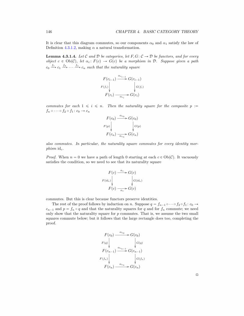
146 CHAPTER 4. BASIC CATEGORY THEORY
It is clear that this diagram commutes, so our components α0 and α1 satisfy the law ofDefinition 4.3.1.2, making α a natural transformation.
Lemma 4.3.1.4. Let C and D be categories, let F,G : C Ñ D be functors, and for everyobject c P ObpCq, let αc : F pcq Ñ Gpcq be a morphism in D. Suppose given a pathc0
f1ÝÑ c1
f2ÝÑ ¨ ¨ ¨
fnÝÑ cn such that the naturality square
F pci´1q
F pfiq
��
αci´1 // Gpci´1q
Gpfiq
��F pciq αci
// Gpciq
commutes for each 1 ď i ď n. Then the naturality square for the composite p :“fn ˝ ¨ ¨ ¨ ˝ f2 ˝ f1 : c0 Ñ cn
F pc0qαc0 //
F ppq
��
Gpc0q
Gppq
��F pcnq αcn
// Gpcnq
also commutes. In particular, the naturality square commutes for every identity mor-phism idc.
Proof. When n “ 0 we have a path of length 0 starting at each c P ObpCq. It vacuouslysatisfies the condition, so we need to see that its naturality square
F pcqαc //
F pidcq
��
Gpcq
Gpidcq
��F pcq
αc
// Gpcq
commutes. But this is clear because functors preserve identities.The rest of the proof follows by induction on n. Suppose q “ fn´1 ˝ ¨ ¨ ¨ ˝f2 ˝f1 : c0 Ñ
cn´1 and p “ fn ˝ q and that the naturality squares for q and for fn commute; we needonly show that the naturality square for p commutes. That is, we assume the two smallsquares commute below; but it follows that the large rectangle does too, completing theproof.
F pc0qαc0 //
F pqq
��
Gpc0q
Gpqq
��F pcn´1q
αcn´1 //
F pfnq
��
Gpcn´1q
Gpfnq
��F pcnq
αcn // Gpcnq
�

4.3. NATURAL TRANSFORMATIONS 147
Example 4.3.1.5. Let C “ D “ r1s be the linear order of length 1, thought of as acategory (by Proposition 4.2.1.17). There are three functors C Ñ D, which we can writeas p0, 0q, p0, 1q, and p1, 1q; these are depicted left to right below.
0‚
� //
f��
0‚
f��
0‚
� //
f��
0‚
f��
0‚z
��f��
0‚
f��
1‚
D
BB
1‚
1‚
� // 1‚1‚
� // 1‚
These are just functors so far. What are the natural transformations say α : p0, 0q Ñp0, 1q? To specify a natural transformation, we must specify a component for each objectin C. In our case α0 : 0 Ñ 0 and α1 : 0 Ñ 1. There is only one possible choice: α0 “ id0and α1 “ f . Now that we have chosen components we need to check the naturalitysquares.
There are three morphisms in C, namely id0, f, id1. By Lemma 4.3.1.4, we need onlycheck the naturality square for f . We write it twice below, once in the abstract notationand once in concrete notation:
F p0q α0 //
F pfq
��
Gp0q
Gpfq
��F p1q
α1// Gp1q
0 id0 //
id0��
0
f
��0
f// 1
This commutes, so α is indeed a natural transformation.Exercise 4.3.1.6. With notation as in Example 4.3.1.5,
a.) how many natural transformations are there p0, 0q Ñ p1, 1q?
b.) how many natural transformations are there p0, 0q Ñ p0, 0q?
c.) how many natural transformations are there p0, 1q Ñ p0, 0q?
d.) how many natural transformations are there p0, 1q Ñ p1, 1q?
♦
Exercise 4.3.1.7. Let List : Set Ñ Set be the functor sending a set X to the set ListpXq oflists with entries in X. We saw above that there is a natural transformation List˝List ÑList given by concatenation.
a.) If someone said “singleton lists give a natural transformation σ from idSet to List”,what might they mean? That is, for a set X, what component σX might they besuggesting?
b.) Do these components satisfy the necessary naturality squares for functions f : X Ñ
Y ?
♦
Exercise 4.3.1.8. Let C and D be categories, and suppose that d P ObpDq is a terminalobject. Consider the functor tduC : C Ñ D that sends each object c P ObpCq to d andeach morphism in C to the identity morphism idd on d.

148 CHAPTER 4. BASIC CATEGORY THEORY
a.) For any other functor F : C Ñ D, how many natural transformations are there F ÑtduC?
b.) Let D “ Set and let d “ t,u. If C “ r1s is the linear order of length 1, andF : C Ñ Set is any functor, what does it mean to give a natural transformationtduC Ñ F?
♦
Application 4.3.1.9. In Figure 3.1 we drew a finite state machine on alphabet Σ “ ta, bu,and in Example 3.1.3.1 we showed the associated action table. It will be reproducedbelow. Imagine this was your model for understanding the behavior of some systemwhen acted on by commands a and b. And suppose that a collaborator tells you that shehas a more refined notion that fits with the same data. Her notion has 6 states ratherthan 3, but it’s “compatible”. What might that mean?
Let’s call the original state machine X and the new model Y .
X:=
State 0
State 1
State 2
a b
a
a
b
b
Y :=
State 0
State 1A
State 2B
b
State 2A State 1B
State 1C
b
b
b
b
a
a
a
a
a
a
b
The action tables for these two machines are:
Original model XID a bState 0 State 1 State 2State 1 State 2 State 1State 2 State 0 State 0
Proposed model YID a bState 0 State 1A State 2AState 1A State 2A State 1BState 1B State 2B State 1CState 1C State 2B State 1BState 2A State 0 State 0State 2B State 0 State 0
How are these models compatible? Looking at the table for Y , if one removes thedistinction between States 1A, 1B, 1C and between States 2A and 2B, then one returnswith the table for X. The table for Y is more specific, but it is fully compatible withtable X. The sense in which it is compatible is precisely the sense defined by there beinga natural transformation.
Recall thatM “ pListpΣq, r s, ` q is a monoid, and that a monoid is simply a categorywith one object, say ObpMq “ tNu (see Section 4.2.1). With Σ “ ta, bu, the monoid Mcan be visualized as follows:
M “ N‚a :: bdd

4.3. NATURAL TRANSFORMATIONS 149
Recall also that a state machine on M is simply a functor M Ñ Set. We thus havetwo such functors, X and Y . A natural transformation α : Y Ñ X would consist of acomponent αm for every object m P ObpMq, such that certain diagrams commute. ButM having only one object, we need only one function αN : Y pNq Ñ XpNq, where Y pNq isthe set of (6) states of Y and XpNq is the set of (3) states of X.
The states of Y have been named so as to make the function αN particularly easy toguess.15 We need to check that two squares commute:
Y pNqαN //
Y paq
��
XpNq
Xpaq
��Y pNq
αN// XpNq
Y pNqαN //
Y pbq
��
XpNq
Xpbq
��Y pNq
αN// XpNq
(4.10)
This can only be checked by going through and making sure certain things match, asspecified by (4.10); we spell it out in gory detail. The columns that should match arethose whose entries are written in blue.
Naturality square for a : NÑ NY pNq [ID] Y paq αN ˝ Y paq αN Xpaq ˝ αNState 0 State 1A State 1 State 0 State 1State 1A State 2A State 2 State 1 State 2State 1B State 2B State 2 State 1 State 2State 1C State 2B State 2 State 1 State 2State 2A State 0 State 0 State 2 State 0State 2B State 0 State 0 State 2 State 0
(4.11)
Naturality square for b : NÑ NY pNq [ID] Y pbq αN ˝ Y pbq αN Xpbq ˝ αNState 0 State 2A State 2 State 0 State 2State 1A State 1B State 1 State 1 State 1State 1B State 1C State 1 State 1 State 1State 1C State 1B State 1 State 1 State 1State 2A State 0 State 0 State 2 State 0State 2B State 0 State 0 State 2 State 0
(4.12)
In reality we need to check that for every morphism in M, such as ra, a, bs, a similardiagram commutes. But this holds automatically. For example (flipping the naturalitysquare sideways for typographical reasons)
Y pNqY paq //
αN
��
Y pNqY paq //
αN
��
Y pNqY pbq //
αN
��
Y pNq
αN
��XpNq
Xpaq// XpNq
Xpaq// XpNq
Xpbq// XpNq
15The function αN : Y pNq Ñ XpNq makes the following assignments: State 0 ÞÑ State 0, State 1A ÞÑ
State 1,State 1B ÞÑ State 1, State 1C ÞÑ State 1, State 2A ÞÑ State 2,State 2B ÞÑ State 2.

150 CHAPTER 4. BASIC CATEGORY THEORY
Since each small square above commutes (as checked by tables 4.11 and 4.12), the bigouter rectangle commutes too.
To recap, the notion of compatibility between Y and X is one that can be checkedand agreed upon by humans, but doing so it is left implicit, and it may be difficult toexplain to an outsider what exactly was agreed to, especially in more complex situations.It is quite convenient to simply claim “there is a natural transformation from Y to X.”
♦♦
Exercise 4.3.1.10. Let F : C Ñ D be a functor. Suppose someone said “the identity onF is a natural transformation from F to itself.”
a.) What might they mean?
b.) If it is somehow true, what are the components of this natural transformation?
♦
Example 4.3.1.11. Let r1s P ObpCatq be the free arrow category described in Exercise4.1.2.31 and let D be any category. To specify a functor F : r1s Ñ D requires thespecification of two objects, F pv1q, F pv2q P ObpDq and a morphism F peq : F pv1q Ñ F pv2qinD. The identity and composition formulas are taken care of once that much is specified.To recap, a functor F : r1s Ñ D is the same thing as a morphism in D.
Thus, choosing two functors F,G : r1s Ñ D is precisely the same thing as choosingtwo morphisms in D. Let us call them f : a0 Ñ a1 and g : b0 Ñ b1, where to be clear wehave f “ F peq, a0 “ F pv0q, a1 “ F pv1q and g “ Gpeq, b0 “ Gpv0q, b1 “ Gpv1q.
A natural transformation α : F Ñ G consists of two components, h0 :“ αv0 : a0 Ñ b0and h1 :“ αv1 : a1 Ñ b1, drawn as dashed lines below:
a0h0 //
f
��
b0
g
��a1
h1
// b1
The condition for α to be a natural transformation is that the above square commutes.In other words, a functor r1s Ñ D is an arrow in D and a natural transformation
between two such functors is just a commutative square in D.Example 4.3.1.12. Recall that to any graph G we can associate the so-called paths-graphPathspGq, as described in Example 4.1.2.22. This is a functor Paths : Grph Ñ Grph.There is also an identity functor idGrph : Grph Ñ Grph. A natural transformationη : idGrph Ñ Paths would consist of a graph homomorphism ηG : idGrphpGq Ñ PathspGqfor every graph G. But idGrphpGq “ G by definition, so we need ηG : G Ñ PathspGq.Recall that PathspGq has the same vertices as G and every arrow in G counts as a path(of length 1). So there is an obvious graph homomorphism from G to PathspGq. It isnot hard to see that the necessary naturality squares commute.Example 4.3.1.13. For any graph G we can associate the paths-graph PathspGq, andnothing stops us from doing that twice to yield a new graph PathspPathspGqq. Let’sthink through what a path of paths in G is. It’s a head-to-tail sequence of arrows inPathspGq, meaning a head-to-tail sequence of paths in G. These composable sequences ofpaths (or “paths of paths”) are the individual arrows in PathspPathspGqq. (The verticesin PathspGq and PathspPathspGqq are the same as those in G, and all source and targetfunctions are as expected.)

4.3. NATURAL TRANSFORMATIONS 151
Clearly, given such a sequence of paths inG, we could compose them to one big path inG with the same endpoints. In other words, there is graph morphism µG : PathspPathspGqq ÑPathspGq, that one might call “concatenation”. In fact, this concatenation extends to anatural transformation
µ : Paths ˝ Paths Ñ Paths
between functors Grph Ñ Grph. In Example 4.3.1.12, we compared a graph to itspaths-graph using a natural transformation idGrph Ñ Paths; here we are making asimilar kind of comparison.Remark 4.3.1.14. In Example 4.3.1.12 we saw that there is a natural transformationsending each graph into its paths-graph. There is a formal sense in which a category isnothing more than a kind of reverse mapping. That is, to specify a category is the samething as to specify a graph G together with a graph homomorphism PathspGq Ñ G. Theformalities involve monads, which we will discuss in Section 5.3.Exercise 4.3.1.15. Let X and Y be sets, and let f : X Ñ Y . There is a functorCX : Grph Ñ Set that sends every graph to the set X and sends every morphismof graphs to the identity morphism idX : X Ñ X. This functor is called the constantfunctor at X. Similarly there is a constant functor CY : Grph Ñ Set.
a.) Use f to construct a natural transformation CX Ñ CY .
b.) What are its components?
♦
Exercise 4.3.1.16. For any graph pV,A, src, tgtq we can extract the set of arrows or the setof vertices. Since each morphism of graphs includes a function between their arrow setsand a function between their vertex sets, we actually have functors Ar : Grph Ñ Setand Ve : Grph Ñ Set.
a.) If someone said “taking source vertices gives a natural transformation from Ar toVe”, what natural transfromation might they be referring to?
b.) What are its components?
c.) If a different person, say from a totally different country, were to say “taking targetvertices also gives a natural transformation from Ar to Ve,” would they also becorrect?
♦
Example 4.3.1.17 (Graph homomorphisms are natural transformations). As discussedabove (see Diagram 4.7), there is a category GrIn for which a functor G : GrIn Ñ Setis the same thing as a graph. Namely, we have
GrIn :“ Ar‚
src //tgt//Ve‚
A natural transformation of two such functors α : G Ñ G1 involves two components,αAr : GpArq Ñ G1pArq and αVe : GpVeq Ñ G1pVeq, and two naturality squares, one forsrc and one for tgt. This is precisely the same thing as a graph homomorphism, asdefined in Definition 3.3.3.1.

152 CHAPTER 4. BASIC CATEGORY THEORY
4.3.2 Vertical and horizontal compositionIn this section we discuss two types of compositions for natural transformations. Theterms vertical and horizontal are used to describe them; these terms come from thefollowing pictures:
αó
C
F
��G //
H
BBDβó
C
F1
!!γ1ó
G1
==D
F2
!!γ2ó
G2
== E
We generally use ˝ to denote both kinds of composition, but if we want to be very clear wewill differentiate as follows: β˝α : F Ñ H for vertical composition, and γ2˛γ1 : F2˝F1 ÝÑG2 ˝ G1 for horizontal composition. Of course, the actual arrangement of things on apage of text does not correlate with verticality or horizontality—these are just names.We will define them more carefully below.
4.3.2.1 Vertical composition of natural transformations
The following proposition proves that functors and natural transformations (using ver-tical composition) form a category.
Proposition 4.3.2.2. Let C and D be categories. There exists a category, called thecategory of functors from C to D and denoted FunpC,Dq, whose objects are the functorsC Ñ D and whose morphisms are the natural transformations,
HomFunpC,DqpF,Gq “ tα : F Ñ G | α is a natural transformationu.
That is, there are identity natural transformations, natural transformations can be com-posed, and the identity and associativity laws hold.
Proof. We showed in Exercise 4.3.1.10 that there for any functor F : C Ñ D, thereis an identity natural transformation idF : F Ñ F (its component at c P ObpCq isidF pcq : F pcq Ñ F pcq).
Given a natural transformation α : F Ñ G and a natural transformation β : GÑ H,we propose for the composite β ˝ α the transformation γ : F Ñ H having componentsβc ˝αc for every c P ObpCq. To see that γ is indeed a natural transformation, one simplyputs together naturality squares for α and β to get naturality squares for β ˝ α.
The associativity and identity laws for FunpC,Dq follow from those holding for mor-phisms in D.
�
Notation 4.3.2.3. We sometimes denote the category FunpC,Dq by DC .
Example 4.3.2.4. Recall from Exercise 4.1.2.38 that there is a functor Ob: Cat Ñ Setsending a category to its set of objects. And recall from Example 4.1.2.35 that thereis a functor Disc : Set Ñ Cat sending a set to the discrete category with that set ofobjects (all morphisms in DiscpSq are identity morphisms). Let P : Cat Ñ Cat be thecomposition P “ Disc ˝ Ob. Then P takes a category and makes a new category withthe same objects but no morphisms. It’s like crystal meth for categories.
4.3. NATURAL TRANSFORMATIONS 153
Let idCat : Cat Ñ Cat be the identity functor. There is a natural transformationi : P Ñ idCat. For any category C, the component iC : P pCq Ñ C is pretty easily under-stood. It is a morphism of categories, i.e. a functor. The two categories P pCq and Chave the same set of objects, namely ObpCq, so our functor is identity on objects; andP pCq has no non-identity morphisms, so nothing else needs be specified.
Exercise 4.3.2.5. Let C “ A‚ be the category with ObpCq “ tAu, and HomCpA,Aq “
tidAu. What is FunpC,Setq? In particular, characterize the objects and the morphisms.♦
Exercise 4.3.2.6. Let n P N and let n be the set with n elements, considered as a discretecategory. 16 In other words, we write n to mean what should really be called Discpnq.Describe the category Funp3, 2q. ♦
Exercise 4.3.2.7. Let 1 denote the discrete category with one object, and let C be anycategory.
a.) What are the objects of Funp1, Cq?
b.) What are the morphisms of Funp1, Cq?
♦
Example 4.3.2.8. Let 1 denote the discrete category with one object (also known as thetrivial monoid). For any category C, we investigate the category D :“ FunpC, 1q. Itsobjects are functors C Ñ 1. Such a functor F assigns to each object in C an object in 1of which there is one; so there is no choice in what F does on objects. And there is onlyone morphism in 1 so there is no choice in what F does on morphisms. The upshot isthat there is only one object in D, let’s call it F , in D, so D is a monoid. What are itsmorphisms?
A morphism α : F Ñ F in D is a natural transformation of functors. For everyc P ObpCq we need a component αc : F pcq Ñ F pcq, which is a morphism 1 Ñ 1 in 1.But there is only one morphism in 1, namely id1, so there is no choice about what thesecomponents should be: they are all id1. The necessary naturality squares commute, soα is indeed a natural transformation. Thus the monoid D is the trivial monoid; that is,FunpC, 1q – 1 for any category C.Exercise 4.3.2.9. Let 0 represent the discrete category on 0 objects; it has no objects andno morphisms. Let C be any category. What is Funp0, Cq? ♦
Exercise 4.3.2.10. Let r1s denote the free arrow category as in Exercise 4.1.2.31, andlet C be the graph indexing category from (4.7). Draw the underlying graph of thecategory Funpr1s, Cq, and then specify which pairs of paths in that graph correspond tocommutative diagrams in Funpr1s, Cq. ♦
16When we have a functor, such as Disc : Set Ñ Cat, we may sometimes say things like “Let Sbe a set, considered as a category” (or in general, given a functor F : C Ñ D, we may say “considerc P ObpCq, taken as an object in D”). What this means is that we want to take ideas and methodsavailable in Cat and use them on our set S. Having our functor Disc lying around, we use it to move Sinto Cat, as DiscpSq P ObpCatq, upon which we can use our intended methods. However, our humanminds get bogged down seeing DiscpSq because it is bulky (e.g. FunpDiscp3q, Discp2qq is harder to readthan Funp3, 2q). So we abuse notation and write S in place of DiscpSq. To add insult to injury, wetalk about S as though it was still a set, e.g. discussing its elements rather than its objects. This kindof conceptual abbreviation is standard practice in mathematical discussion because it eases the mentalburden for experts, but when one says “Let S be an X considered as a Y ” the other may always ask,“How again are you considering X’s to be Y ’s?” and expect a functor .

154 CHAPTER 4. BASIC CATEGORY THEORY
4.3.2.11 Natural isomorphisms
Let C and D be categories. We have defined a category FunpC,Dq whose objects arefunctors C Ñ D and whose morphisms are natural transformations. What are theisomorphisms in this category?
Lemma 4.3.2.12. Let C and D be categories and let F,G : C Ñ D be functors. A naturaltransformation α : F Ñ G is an isomorphism in FunpC,Dq if and only if the componentαc : F pcq Ñ Gpcq is an isomorphism for each object c P ObpCq. In this case α is called anatural isomorphism.
Proof. First suppose that α is an isomorphism with inverse β : GÑ F , and let βc : Gpcq ÑF pcq denote its c component. We know that α ˝ β “ idG and β ˝ α “ idF . Using thedefinitions of composition and identity given in Proposition 4.3.2.2, this means that forevery c P ObpCq we have αc ˝ βc “ idGpcq and βc ˝ αc “ idF pcq; in other words αc is anisomorphism.
Second suppose that each αc is an isomorphism with inverse βc : Gpcq Ñ F pcq. Weneed to see that these components assemble into a natural transformation; i.e. for everymorphism h : cÑ c1 in C the right-hand square
F pcq
XF phq
��
αc // Gpcq
Gphq
��F pc1q
αc1
// Gpc1q
Gpcq
?Gphq
��
βc // F pcq
F phq
��Gpc1q
βc1
// F pc1q
commutes. We know that the left-hand square commutes because α is a natural trans-formation; we have labeled each square with a ? or a X accordingly. In the followingdiagram we want to show that the left-hand square commutes. We know that the middlesquare commutes.
Gpcq
idGpcq
&&
?Gphq
��
βc // F pcq
XF phq
��
αc // Gpcq
?Gphq
��
βc // F pcq
F phq
��Gpc1q
βc1
// F pc1qαc1
//
idF pc1q
88Gpc1q
βc1
// F pc1q
To complete the proof we need only to show that F phq ˝ βc “ βc1 ˝ Gphq. This can beshown by a “diagram chase.” We go through it symbolically, for demonstration.
F phq ˝ βc “ βc1 ˝ αc1 ˝ F phq ˝ βc “ βc1 ˝Gphq ˝ αc ˝ βc “ βc1 ˝Gphq.
�
Exercise 4.3.2.13. Recall from Application 4.3.1.9 that a finite state machine on alphabetΣ can be understood as a functor M Ñ Set, where M “ ListpΣq is the free monoid

4.3. NATURAL TRANSFORMATIONS 155
generated by Σ. In that example we also discussed how natural transformations providea nice language for changing state machines. Describe what kinds of changes are madeby natural isomorphisms. ♦
4.3.2.14 Horizontal composition of natural transformations
Example 4.3.2.15 (Whiskering). Suppose that M “ Listpa, bq and M1 “ Listpm,n, pqare free monoids, and let F : M1 Ñ M be given by sending rms ÞÑ ras, rns ÞÑ rbs, andrps ÞÑ rb, a, as. An application of this might be if the sequence rb, a, as was commonlyused in practice and one wanted to add a new button just for that sequence.
Recall Application 4.3.1.9. Let X : MÑ Set and Y : MÑ Set be the functors, andlet α : Y Ñ X be the natural transformation found there. We reproduce them here:
State 0
State 1
State 2
a b
a
a
b
b
State 0
State 1A
State 2B
b
State 2A State 1B
State 1C
b
b
b
b
a
a
a
a
a
a
b
Original model X : M Ñ SetID a bState 0 State 1 State 2State 1 State 2 State 1State 2 State 0 State 0
Proposed model Y : M Ñ SetID a bState 0 State 1A State 2AState 1A State 2A State 1BState 1B State 2B State 1CState 1C State 2B State 1BState 2A State 0 State 0State 2B State 0 State 0
We can compose X and Y with F as in the diagram below
M1 F //M
Y
((
X
66αó Set
to get functors Y ˝ F and X ˝ F , both of type M1 Ñ Set. What would these be? 17
X ˝ F
ID m n pState 0 State 1 State 2 State 1State 1 State 2 State 1 State 0State 2 State 0 State 0 State 2
Y ˝ F
ID m n pState 0 State 1A State 2A State 1AState 1A State 2A State 1B State 0State 1B State 2B State 1C State 0State 1C State 2B State 1B State 0State 2A State 0 State 0 State 2AState 2B State 0 State 0 State 2A
The map α is what sent both State 1A and State 1B in Y to State 1 in X, andso on. We can see that “the same α works now:” the p column of the table respectsthat mapping. But α was a natural transformation Y Ñ X where as we need a naturaltransformation Y ˝ F Ñ X ˝ F . This is called whiskering. It is a kind of horizontalcomposition of natural transformation.
17The p-column comes from applying b then a then a, as specified above by F .

156 CHAPTER 4. BASIC CATEGORY THEORY
Definition 4.3.2.16 (Whiskering). Let B, C,D, and E be categories, let G1, G2 : C Ñ Dbe functors, and let α : G1 Ñ G2 a natural transformation. Suppose that F : B Ñ C(respectively H : D Ñ E) is a functor, depicted below:
B F // C αó
G1""
G2
??D
¨
˚
˚
˝
respectively, C αó
G1""
G2
??DH // E
˛
‹
‹
‚
,
Then the pre-whiskering of α by F , denoted α ˛ F : G1 ˝ F Ñ G2 ˝ F (respectively, thepost-whiskering of α by H, denoted H ˛ α : H ˝G1 Ñ H ˝G2) is defined as follows.
For each b P ObpBq the component pα ˛ F qb : G1 ˝ F pbq Ñ G2 ˝ F pbq is defined tobe αF pbq. (Respectively, for each c P ObpCq the component pH ˛ αqc : H ˝ G1pcq ÑH ˝ G2pcq is defined to be Hpαcq.) Checking that the naturality squares (in each case)is straightforward.
The rest of this section can safely be skipped; I include it only for my own sense ofcompleteness.
Definition 4.3.2.17 (Horizontal composition of natural transformations). Let B, C, andD be categories, let F1, F2 : B Ñ C and G1, G2 : C Ñ D be functors, and let α : F1 Ñ F2and β : G1 Ñ G2 be natural transformations, as depicted below:
B αó
F1!!
F2
?? C βó
G1""
G2
??D
By pre- and post-whiskering in one order or the other we get the following diagram
G1 ˝ F1G1˛α //
β˛F1
��
G1 ˝ F2
β˛F2
��G2 ˝ F1
G2˛α// G2 ˝ F2
It is straightforward to show that this diagram commutes, so we can take the compositionto be our definition of the horizontal composition
β ˛ α : G1 ˝ F1 Ñ G2 ˝ F2.
Remark 4.3.2.18. Whiskering a natural transformation α with a functor F is the samething as horizontally composing α with the identity natural transformation idF . Thisis true for both pre- and post- whiskering. For example in the notation of Definition4.3.2.16 we have
α ˛ F “ α ˛ idF and H ˛ α “ idH ˛ α.Remark 4.3.2.19. All of the above is somehow similar to the world of paths inside adatabase schema S, as seen in Definition 3.5.2.3. Indeed, a congruence on the paths of Sis an equivalence relation that is closed under composition. The equivalence relation partis analogous to the fact that natural transformations can be composed vertically. Theclosure under composition part (Properties (3) and (4) in Definition 3.5.2.3) is analogousto pre- and post whiskering. See also Lemma 3.5.2.5.
This is being mentioned only as a curiosity and a way for the reader to draw connec-tions, not with any additional purpose at this time.

4.3. NATURAL TRANSFORMATIONS 157
Theorem 4.3.2.20.
α1ó β1ó
C
F1
��F2 //
F3
BBD
G1
��G2 //
G3
BBEα2ó β2ó
Given a setup of categories, functors, and natural transformations as above, we have
pβ2 ˝ β1q ˛ pα2 ˝ α1q “ pβ2 ˛ α2q ˝ pβ1 ˛ α1q.
Proof. One need only observe that each square in the following diagram commutes, sofollowing the outer path pβ2 ˝ β1q ˛ pα2 ˝ α1q yields the same morphism as following thediagonal path ; pβ2 ˛ α2q ˝ pβ1 ˛ α1q:
G1F1G1˛α1 //
β1˛F1
��
G1F2G1˛α2 //
β1˛F2
��
G1F3
β1˛F3
��G2F1
G2˛α1 //
β2˛F1
��
G2F2G2˛α2 //
β2˛F2
��
G2F3
β2˛F3
��G3F1
G3˛α1
// G3F2G3˛α2
// G3F3
�
4.3.3 The category of instances on a database schemaIn Section 4.2.2 we showed that schemas are presentations of categories, and we willshow in Section 4.4 that in fact the category of schemas is equivalent to the categoryof categories. In this section we therefore take license to blur the distinction betweenschemas and categories.
If C is a schema, i.e. a category, then as we discussed in Section 4.2.2.5, an instanceon C is a functor I : C Ñ Set. But now we have a notion beyond categories and functors,namely that of natural transformations. So we make the following definition.
Definition 4.3.3.1. Let C be a schema (or category). The category of instances on C,denoted C–Set, is FunpC,Setq. Its objects are C-instances (i.e. functors C Ñ Setq andits morphisms are natural transformations.
Remark 4.3.3.2. One might object to Definition 4.3.3.1 on the grounds that databaseinstances should not be infinite. This is a reasonable perspective, so it is a pleasant factthat the above definition can be modified easily to accomodate it. The subcategory Fin(see Example 4.1.1.4) of finite sets can be substituted for Set in Definition 4.3.3.1. Onecould define the category of finite instances on C as C ´ Fin “ FunpC,Finq. Almost allof the ideas in this book will make perfect sense in C ´ Fin.
Natural transformations should serve as some kind of morphism between instances onthe same schema. How are we to interpret a natural transformation α : I Ñ J betweendatabase instances I, J : C Ñ Set?

158 CHAPTER 4. BASIC CATEGORY THEORY
Our first clue comes from Application 4.3.1.9. There we considered the case ofa monoid M, and we thought about a natural transformation between two functorsX,Y : M Ñ Set, considered as different finite state machines. The notion of naturaltransformation captured the idea of one model being a refinement of another. This samekind of idea works for databases with more than one table (categories with more thanone object), but the whole thing is a bit opaque. Let’s work it through slowly.
Example 4.3.3.3. Let us consider the terminal schema, 1 – ‚Grapes . An instance is afunctor 1 Ñ Set and it is easy to see that this is the same thing as just a set. A naturaltransformation α : I Ñ J is a function from set I to set J . In the standard table view,we might have I and J as below:
Grapes pIqIDGrape 1Grape 3Grape 4
Grapes pJqIDJan1-01Jan1-02Jan1-03Jan1-04Jan3-01Jan4-01Jan4-02
There are 343 natural transformations I Ñ J . Perhaps some of them make more sensethan others; e.g. we could hope that the numbers in I corresponded to the numbers afterthe dash in J , or perhaps to what seems to be the date in January. But it could be thatthe rows in J correspond to batches, and all three grapes in I are part of the first batchon Jan-1. The notion of natural transformation is a mathematical one.
Exercise 4.3.3.4. Recall the notion of set-indexed sets from Definition 2.7.6.12. Let A bea set, and come up with a schema A such that instances on A are A-indexed sets. Is ourcurrent notion of morphism between instances (i.e. natural transformations) well-alignedwith the above definition of “mapping of A-indexed sets”? ♦
For a general schema (or category) C, let us think through what a morphism α : I Ñ Jbetween instances I, J : C Ñ Set is. For each object c P ObpCq there is a componentαc : Ipcq Ñ Jpcq. This means that just like in Example 4.3.3.3, there is for each table ca function from the rows in I’s manifestation of c to the rows in J ’s manifestation of c.So to make a natural transformation, such a function has to be specified table by table.But then we have to contend with naturality squares, one for every arrow in C. Arrowsin C correspond to foreign key columns in the database. The naturality requirement wasalready covered in Application 4.3.1.9 (and see especially how (4.10) is checked in (4.11)and (4.12)).
Example 4.3.3.5. We saw in Section 4.2.1.20 that graphs can be regarded as functorsG Ñ Set, where G – GrIn is the “schema for graphs” shown here:
G :“ Arrow‚
src //tgt//Vertex‚
A database instance I : G Ñ Set on G consists of two tables. Here is an example

4.3. NATURAL TRANSFORMATIONS 159
instance:
I :“ ‚vf // ‚w
h
==
g
##‚x
Arrow pIq
ID src tgtf v wg w xh w x
Vertex pIq
IDvwx
To discuss natural transformations, we need two instances. Here is another, J : G Ñ Set,
J :“
q‚
i // r‚
j
s‚
k
__` // t‚
u‚
Arrow pJq
ID src tgti q rj r sk s r` s t
Vertex pJq
IDqrstu
To give a natural transformation α : I Ñ J , we give two components: one for arrowsand one for vertices. We need to say where each vertex in I goes in J and we need tosay where each arrow in I goes in J . The naturality squares insist that if we specifythat g ÞÑ j, for example, then we better specify thatw ÞÑ r and that x ÞÑ s. What acomputer is very good at, but a human is fairly slow at, is checking that a given pair ofcomponents (arrows and vertices) really is natural.
There are 8000 ways to come up with component functions αArrow and αVertex, butprecisely four natural transformations, i.e. four graph homomorphisms, I Ñ J ; the other7996 are haphazard flingings of arrows to arrows and vertices to vertices without anyregard to sources and targets. We briefly describe the four now.
First off, nothing can be sent to u because arrows must go to arrows and u touchesno arrows. If we send v ÞÑ q then f must map to i, and w must map to r, and both gand h must map to j, and x must map to s. If we send v ÞÑ r then there are two choicesfor g and h. If we send v ÞÑ s then there’s one way to obtain a graph morphism. If wetry to send v ÞÑ? t, we fail. All of this can be seen by staring at the tables rather thanat the pictorial representations of the graphs; the human eye understands these picturesbetter, but the computer understands the tables better.Exercise 4.3.3.6. If I, J : G Ñ Set are as in Example 4.3.3.5, how many natural trans-formations are there J Ñ I? ♦
Exercise 4.3.3.7. Let YA : G Ñ Set denote the instance below:
Arrow pYAq
ID src tgta v0 v1
Vertex pYAq
IDv0v1
Let I : G Ñ Set be as in Example 4.3.3.5.
a.) How many natural transformations are there YA Ñ I?
b.) With J as above, how many natural transformations are there YA Ñ J?
c.) Do you have any conjecture about the way natural transformations YA Ñ X behavefor arbitrary graphs X : G Ñ Set?
160 CHAPTER 4. BASIC CATEGORY THEORY
♦
In terms of databases, this notion of instance morphism I Ñ J is fairly benign. Forevery table its a mapping from the set of rows in I’s version of the table to J ’s versionof the table, such that all the foreign keys are respected. We will see that this notion ofmorphism has excellent formal properties, so that projections, unions, and joins of tables(the typical database operations) would be predicted to be “obviously interesting” by acategory theorist who had no idea what a database was. 18
However, something is also missing from the natural transformation picture. A veryimportant occurrence in the world of databases is the update. Everyone can understandthis: a person makes a change in one of the tables, like changing your address fromCambridge, MA to Hereford, UK. Most such arbitrary changes of database instance arenot “natural”, in that the new linking pattern is incompatible with the old.
It is interesting to consider how updates of C-instances should be understood categorytheoretically. We might want a category UpdC whose objects are C-instances and whosemorphisms are updates. But then what is the composition formula? Is there a uniquemorphism I Ñ J whenever J can be obtained as an update on I? Because in that case,we would be defining UpdC to be the indiscrete category on the set of C-instances (seeExample 4.3.4.3).Exercise 4.3.3.8. Research project: Can you come up with a satisfactory way to modeldatabase updates category-theoretically? Let N be the category
rNs :“ 0‚ // 1‚ // 2‚ // ¨ ¨ ¨
representing a discrete timeline. A place to start might be to use something like the slicecategory Cat{rNs where the fiber over each object in N is a snapshot of the database intime. Can you make this work? ♦
4.3.4 Equivalence of categoriesWe have a category Cat of categories, and in every category there is a notion of isomor-phism between objects: one morphism each way, such that each round-trip compositionis the identity. An isomorphism in Cat, therefore, takes place between two categories,say C and D: it is a functor F : C Ñ D and a functor G : D Ñ C such that G ˝ F “ idCand F ˝G “ idD.
It turns out that categories are often similar enough to be considered equivalentwithout being isomorphic. For this reason, the notion of isomorphism is considered “toostrong” to be useful for categories. The feeling to a category theorist might be akin tosaying that two material samples are the same if there is an atom-by-atom matching, orthat two words are the same if they are written in the same font, of the same size, bythe same person, in the same state of mind.
As reasonable as isomorphism is as a notion in most categories, it fails to be the“right notion” about categories. The reason is that in categories there are objects andmorphisms, whereas when we talk about categories, we have categories and functors, plusnatural transformations. These serve as mappings between mappings, and this is notpart of the structure of an ordinary category. In cases where a category C does havesuch mappings between mappings, it is often a “better notion” if we take that extra
18More precisely, given a functor between schemas F : C Ñ D, the pullback ∆F : D–Set Ñ C–Set, itsleft ΣF and its right adjoint ΠF constitute these important queries. See Section 5.1.4.

4.3. NATURAL TRANSFORMATIONS 161
structure into account, like we will for categories. This whole subject leads us to thestudy of 2-categories (or n-categories, or 8-categories), which we do not discuss in thisbook. See, for example, [Le1] for an introduction.
Regardless, our purpose now is to explain this “good notion” of sameness for cat-egories, namely equivalences of categories, which appropriately take natural transfor-mations into account. Instead of “functors going both ways with round trips equal toidentity”, which is required in order to be an isomorphism of categories, equivalence ofcategories demands “functors going both ways with round trips isomorphic to identity”.
Definition 4.3.4.1 (Equivalence of categories). Let C and C1 be categories. A functorF : C Ñ C1 is called an equivalence of categories, and denoted F : C »
ÝÑ C1, 19 if there existsa functor F 1 : C1 Ñ C and natural isomorphisms α : idC
–ÝÑ F 1 ˝F and α1 : idC1
–ÝÑ F ˝F 1.
In this case we say that F and F 1 are mutually inverse equivalences.
Unpacking a bit, suppose we are given functors F : C Ñ C1 and F 1 : C1 Ñ C. We wantto know something about the roundtrips on C and on C1; we want to know the samekind of information about each roundtrip, so let’s concentrate on the C side. We wantto know something about F 1 ˝ F : C Ñ C, so let’s name it i : C Ñ C; we want to knowthat i is a natural isomorphism. That is, for every c P ObpCq we want an isomorphismαc : c –
ÝÑ ipcq, and we want to know that these isomorphisms are picked carefully enoughthat given g : cÑ c1 in C, the choice of isomorphisms for c and c1 are compatible,
cαc //
g
��
ipcq
ipgq
��c1
αc1
// ipc1q.
To be an equivalence, the same has to hold for the other roundtrip, i1 “ F ˝F 1 : C1 Ñ C1.Exercise 4.3.4.2. Let C and C1 be categories. Suppose that F : C Ñ C1 is an isomorphismof categories.
a.) Is it an equivalence of categories?
b.) What are the components of α and α1 (with notation as in Definition 4.3.4.1)?
♦
Example 4.3.4.3. Let S be a set and let S ˆ S Ď S ˆ S be the complete relation onS, which is a preorder KS . Recall from Proposition 4.2.1.17 that we have a functori : PrO Ñ Cat, and the resulting category ipKSq is called the indiscrete category on S;it has objects S and a single morphism between every pair of objects. Here is a pictureof Kt1,2,3u:
1‚
��))
��
2‚ qqii
��3‚DD
AAQQ
19The notation » has already been used for equivalences of paths in a schema. We do not mean toequate these ideas; we are just reusing the symbol. Hopefully no confusion will arise.

162 CHAPTER 4. BASIC CATEGORY THEORY
It is easy check that K1, the indiscrete category on one element, is isomorphic to 1,the discrete category on one object, also known as the terminal category (see Exercise4.1.2.37). The category 1 consists of one object, its identity morphism, and nothing else.
The only way that KS can be isomorphic to 1 is if S has one element. 20 On theother hand, there is an equivalence of categories
KS » 1
for every set S ‰ H.In fact, there are many such equivalences, one for each element of S. To see this,
let S be a nonempty set and choose an element s0 P S. For every s P S, there is aunique isomorphism ks : s –
ÝÑ s0 in KS . Let F : KS Ñ 1 be the only possible functor(see Exercise 4.1.2.37), and let F 1 : 1 Ñ KS send the unique object in 1 to the object s0.
Note that F 1 ˝ F “ id1 : 1 Ñ 1 is the identity, but that F ˝ F 1 : KS Ñ KS sendseverything to s0. Let α “ id1 and define α1 : idKS
Ñ F ˝ F 1 by α1s “ ks. Note that α1s isan isomorphism for each s P ObpKSq, and note that α1 is a natural transformation (hencenatural isomorphism) because every possible square commutes in KS . This completesthe proof, initiated in the paragraph above, that the category KS is equivalent to 1 forevery nonempty set S, and that this fact can be witnessed by any element s0 P S.Example 4.3.4.4. Consider the category FLin, described in Example 4.1.1.11, of finitenonempty linear orders. For every natural number n P N, let rns P ObpFLinq denote thelinear order shown in Example 3.4.1.7. Define a category ∆ whose objects are given byObp∆q “ trns | n P Nu and with Hom∆prms, rnsq “ HomFLinprms, rnsq. The differencebetween FLin and ∆ is only that objects in FLin may have “funny labels”, e.g.
5‚ // x‚ // “Sam”
‚
whereas objects in ∆ all have standard labels, e.g.
0‚ // 1‚ // 2‚
Clearly FLin is a much larger category, and yet feels like it is “pretty much the sameas” ∆. Justly, they are equivalent, FLin » ∆.
The functor F 1 : ∆ Ñ FLin is the inclusion; the functor F : FLin Ñ ∆ sends everyfinite nonempty linear order X P ObpFLinq to the object F pXq :“ rns P ∆, whereObpXq – t0, 1, . . . , nu. For each such X there is a unique isomorphism αX : X –
ÝÑ rns,and these fit together into 21 the required natural isomorphism idFLin Ñ F 1 ˝ F . Theother natural isomorphism α1 : id∆ Ñ F ˝ F 1 is the identity.Exercise 4.3.4.5. Recall from Definition 2.1.2.16 that a set X is called finite if thereexists a natural number n P N and an isomorphism of sets X Ñ n. Let Fin denote thecategory whose objects are the finite sets and whose morphisms are the functions. LetS denote the category whose objects are the sets n and whose morphisms are again thefunctions. For every object X P ObpFinq there exists an isomorphism pX : X Ñ n forsome unique object n P ObpSq. Find an equivalence of categories Fin »
ÝÑ S. ♦
20One way to see this is that by Exercise 4.1.2.38, we have a functor Ob: Cat Ñ Set, and we knowby Exercise 4.1.2.24 that functors preserve isomorphisms, so an isomorphism between categories mustrestrict to an isomorphism between their sets of objects. The only sets that are isomorphic to 1 haveone element.
21The phrase “these fit together into” is suggestive shorthand for, and thus can be replaced with, thephrase “the naturality squares commute for these components, so together they constitute”.

4.3. NATURAL TRANSFORMATIONS 163
Exercise 4.3.4.6. We say that two categories C and D are equivalent if there exists anequivalence of categories between them. Show that the relation of “being equivalent” isan equivalence relation on ObpCatq. ♦
Example 4.3.4.7. Consider the group Z2 :“ pt0, 1u, 0,`q, where 1`1 “ 0. As a category,Z2 has one object N and two morphisms, namely 0, 1, such that 0 is the identity. SinceZ2 is a group, the morphism 1: NÑ N must have an inverse x, meaning 1` x “ 0, andx “ 1 is the only solution.
The point is that the morphism 1 in Z2 is an isomorphism. Let C “ 1 be the terminalcategory as in Exercise 4.1.2.37. One might accidentally believe that C is equivalentto Z2, but this is not the case! The argument in favor of the accidental belief is thatwe have unique functors F : Z2 Ñ C and F 1 : C Ñ Z2 (and this is true); the roundtripF ˝ F 1 : C Ñ C is the identity (and this is true); and for the roundtrip F 1 ˝ F : Z2 Ñ Z2both morphisms in Z2 are isomorphisms, so any choice of morphism αN : NÑ F 1 ˝ F pNqwill be an isomorphism (and this is true). The problem is that no such αN will be anatural transformation.
When we roundtrip F 1 ˝ F : Z2 Ñ Z2, the image of 1 : NÑ N is F 1 ˝ F p1q “ 0 “ idN.So the naturality square for the morphism 1 looks like this:
NαN //
1��
N
0“F 1˝F p1q��
NαN// N
where we still haven’t decided whether we want αN to be 0 or 1. Unfortunately, neitherchoice works (i.e. for neither choice will the diagram commute) because x` 1 ‰ x` 0 inZ2.
Definition 4.3.4.8 (Skeleton). Let C be a category. We saw in Lemma 4.1.1.21 thatthe relation of “being isomorphic” is an equivalence relation – on ObpCq. An election inC is a choice E of the following sort:
• for each –-equivalence class S Ď ObpCq a choice of object sE P S, called the electedobject for S, and
• for each object c P ObpCq a choice of isomorphism ic : sE Ñ c and jc : cÑ sE withic ˝ jc “ idc and jc ˝ ic “ idsE
, where sE is an elected object (depending on c).
Given an election E in C, there is a category called the E-elected skeleton of C, denotedSkelEpCq, whose objects are the elected objects and whose morphisms s Ñ t for anyelected objects s, t P ObpCq are given by HomSkelEpCqps, tq “ HomCps, tq. Any objectc P ObpCq is isomorphic to a unique elected object sE ; we refer to sE as the elected rep-resentative of c; we refer to the isomorphisms ic and jc as the representing isomorphismsfor c.
Proposition 4.3.4.9. Let C be a category and let E be an election in C. There is anequivalence of categories
SkelEpCq » C.
Proof. The functor F 1 : SkelEpCq Ñ C is the inclusion. The functor F : C Ñ SkelEpCqsends each object in C to its elected representative. Given objects c, c1 P ObpCq with
164 CHAPTER 4. BASIC CATEGORY THEORY
elected representatives s, t respectively, and given a morphism g : cÑ c1 in C, let ic, jc, ic1 ,and jc1 be the representing isomorphisms, and define F pgq : sÑ t to be the composite
sic // c
g // c1jc1 // t.
This is functorial because it sends the identity to the identity and F pg˝g1q “ F pgq˝F pg1q.The composite F ˝F 1 : SkelEpCq Ñ SkelEpCq is the identity. For each c P ObpCq define
αc : c –ÝÑ F 1 ˝ F pcq by αc :“ jc. Given g : cÑ c1 the required naturality square is shown
to the left below:c
jc //
g
��
?
sic //
F 1˝F pgq
��
c
g
��c1
j1c
// t c1j1c
oo
The right-hand part commutes by definition of F and F 1; i.e. j1 ˝ g ˝ ic “ F 1 ˝F pgq. Theleft-hand square commutes because ic ˝ jc “ idc.
�
Definition 4.3.4.10. A skeleton of C is a category S, equivalent to C, such that for anytwo objects s, s1 P ObpSq, if s – s1 then s “ s1.
Exercise 4.3.4.11. Let P be a preorder (considered as a category).
a.) If P 1 is a skeleton of P, is it a partial order?
b.) Is every partial order the skeleton of some preorder?
♦
Definition 4.3.4.12 (Full and faithful functors). Let C and D be categories, andlet F : C Ñ D be a functor. For any two objects c, c1 P ObpCq, we have a functionHomF pc, c
1q : HomCpc, c1q Ñ HomDpF pcq, F pc
1qq guaranteed by the definition of functor.We say that F is a full functor if HomF pc, c
1q is surjective for every c, c1. We say thatF is a faithful functor if HomF pc, c
1q is injective for every c, c1. We say that F is a fullyfaithful functor if HomF pc, c
1q is bijective for every c, c1.
Exercise 4.3.4.13. Let 1 and 2 be the discrete categories on one and two objects, respec-tively. There is only one functor 2 Ñ 1.
a.) Is it full?
b.) Is it faithful?
♦
Exercise 4.3.4.14. Let 0 denote the empty category, and let C be any category. There isa unique functor F : 0 Ñ C.
a.) For general C will F be full?
b.) For general C will F be faithful?
c.) For general C will F be an equivalence of categories?

4.4. CATEGORIES AND SCHEMAS ARE EQUIVALENT, CAT » SCH 165
♦
Proposition 4.3.4.15. Let C and C1 be categories and let F : C Ñ C1 be an equivalenceof categories. Then F is fully faithful.
Proof. Suppose F is an equivalence, so we can find a functor F 1 : C1 Ñ C and naturalisomorphisms α : idC
–ÝÑ F 1 ˝ F and α1 : idC1
–ÝÑ F ˝ F 1. We need to know that for any
objects c, d P ObpCq, the map
HomF pc, dq : HomCpc, dq Ñ HomC1pFc, Fdq
is bijective. Consider the following diagram
HomCpc, dqHomF pc,dq //
α
&&
HomC1pFc, Fdq
α1
((
HomF 1 pFc,Fdq
��HomCpF
1Fc, F 1FdqHomF pF
1Fc,F 1Fdq
// HomC1pFF1Fc, FF 1Fdq
The fact that α is bijective implies that the vertical function is surjective. The fact thatα1 is bijective implies that the vertical function is injective, so it is bijective. This impliesthat HomF pc, dq is bijective as well.
�
Exercise 4.3.4.16. Let Z2 be the group (as category) from Example 4.3.4.7. Are thereany fully faithful functors Z2 Ñ 1? ♦
4.4 Categories and schemas are equivalent, Cat » SchPerhaps it is intuitively clear that schemas are somehow equivalent to categories, and inthis section we make that precise. The basic idea was already laid out in Section 4.2.2.
4.4.1 The category Sch of schemasRecall from Definition 3.5.2.6 that a schema consists of a pair C :“ pG,»q, where G “pV,A, src, tgtq is a graph and » is a congruence, meaning a kind of equivalence relationon the paths in G (see Definition 3.5.2.3. If we think of a schema as being analogous to acategory, what should fulfill the role of functors? That is, what are to be the morphismsin Sch?
Unfortunately, ones first guess may give the wrong notion if we want an equivalenceSch » Cat. Since objects in Sch are graphs with additional structure, one might imaginethat a morphism C Ñ C1 in Sch should be a graph homomorphism (as in Definition3.3.3.1) that preserves said structure. But graph homomorphisms require that arrows besent to arrows, whereas we are more interested in paths than in individual arrows—thearrows are merely useful for presentation.
If instead we define morphisms between schemas to be maps that send paths in C topaths in C1, subject to the requirements that path endpoints, path concatenations, andpath equivalences are preserved, this will turn out to give the correct notion. And since

166 CHAPTER 4. BASIC CATEGORY THEORY
a path is a concatenation of its arrows, it suffices to give a function F from the arrows ofC to the paths of C1, which automatically takes care of the first two requirements above;we must only take care that F preserves path equivalences.
Recall from Examples 4.1.2.22 and 4.3.1.13 the paths-graph functor Paths : Grph ÑGrph, the paths of paths functor Paths ˝ Paths : Grph Ñ Grph, and the naturaltransformations for any graph G,
ηG : GÑ PathspGq and µG : PathspPathspGqq Ñ PathspGq. (4.13)
The function ηG spells out the fact that every arrow in G counts as a path in G, and thefunction µG spells out the fact that a head-to-tail sequence of paths (a path of paths) inG can be concatenated to a single path in G.
Exercise 4.4.1.1. Let r2s denote the graph 0‚Ñ
1‚Ñ
2‚, and let Loop denote the unique graph
having one vertex and one arrow (pictured in Diagram (3.17)).
a.) Find a graph homomorphism f : r2s Ñ PathspLoopq that is injective on arrows(i.e. such that no two arrows in the graph r2s are sent by f to the same arrowin PathspLoopq).
b.) The graph r2s has 6 paths, so Pathspr2sq has 6 arrows. What are the images of thesearrows under the graph homomorphism Pathspfq : Pathspr2sq Ñ PathspPathspLoopqq?
♦
We are almost ready to give the definition of schema morphism, but before we do, let’sreturn to our original idea. Given graphs G,G1 (underlying schemas C, C1) we originallywanted a function from the paths in G to the paths in G1, but we realized it was moreconcise to speak of a function from arrows in G to paths in G1. How do we get backwhat we originally wanted from the concise version? Given a graph homomorphismf : G Ñ PathspG1q, we use (4.13) to form the following composition, which we denotesimply by Pathsf : PathspGq Ñ PathspG1q:
PathspGqPathspfq // PathspPathspG1qq
µG1 // PathspG1q (4.14)
This says that given a function from arrows in G to paths in G1, a path in G becomesa path of paths in G1, which can be concatenated to a path in G1. This simply andprecisely spells out our intuition.
Definition 4.4.1.2 (Schema morphism). LetG “ pV,A, src, tgtq andG1 “ pV 1, A1, src1, tgt1qbe graphs, and let C “ pG,»Gq and C1 “ pG1,»G1q be schemas. A schema morphism Ffrom C to D, denoted F : C Ñ D is a graph homomorphism 22
F : GÑ PathspG1q
that satisfies the following condition for any paths p and q in G:
if p »G q then PathsF ppq »G1 PathsF pqq. (4.15)
Two schema morphisms E,F : C Ñ C1 are considered identical if they agree on vertices(i.e. E0 “ F0) and if, for every arrow f in G, there is a path equivalence in G1
E1pfq »G1 F1pfq.
22By Definition 3.3.3.1, a graph homomorphism F : G Ñ PathspG1q will consist of a vertex partF0 : V Ñ V 1 and an arrows part F1 : E Ñ PathpG1q. See also Definition 3.3.2.1.

4.4. CATEGORIES AND SCHEMAS ARE EQUIVALENT, CAT » SCH 167
We now define the category of schemas, denoted Sch, to be the category whose objectsare schemas as in Definition 3.5.2.6 and whose morphisms are schema morphisms definedas above. The identity morphism on schema C “ pG,»Gq is the schema morphismidC :“ ηG : G Ñ PathspGq as defined in Equation (4.13). We need only understandhow to compose schema morphisms F : C Ñ C1 and F 1 : C1 Ñ C2. On objects theircomposition is obvious. Given an arrow in C, it is sent to a path in C1; each arrow in thatpath is sent to a path in C2. We then have a path of paths which we can concatenate(via µG2 : PathspPathspG2qq Ñ PathspG2q as in 4.13) to get a path in C2 as desired.
Slogan 4.4.1.3.
“ A schema morphism sends vertices to vertices, arrows to paths, and pathequivalences to path equivalences. ”
Example 4.4.1.4. Let r2s be the linear order graph of length 2, pictured to the left, andlet C denote the schema pictured to the right below:
r2s :“ 0‚
f1 // 1‚f2 // 2‚ C :“
a‚
g //
i��
b‚
h��c‚
We impose on C the path equivalence declaration rg, hs » ris and show that in this caseC and r2s are isomorphic in Sch. We have a schema morphism F : r2s Ñ C sending0 ÞÑ a, 1 ÞÑ b, 2 ÞÑ c, and sending each arrow in r2s to an arrow in C. And we havea schema morphism F 1 : C Ñ r2s which reverses this mapping on vertices; note thatF 1 must send the arrow i in C to the path rf1, f2s in r2s, which is ok! The roundtripF 1 ˝ F : r2s Ñ r2s is identity. The roundtrip F ˝ F 1 : C Ñ C may look like it’s notthe identity; indeed it sends vertices to themselves but it sends i to the path rg, hs.But according to Definition 4.4.1.2, this schema morphism is considered identical to idCbecause there is a path equivalence idCpiq “ ris » rg, hs “ F ˝ F 1piq.
Exercise 4.4.1.5. Consider the schema r2s and the schema C pictured above, except wherethis time we do not impose any path equivalence declarations on C, so rg, hs fi ris in ourcurrent version of C.
a.) How many schema morphisms are there r2s Ñ C that send 0 to a?
b.) How many schema morphisms are there C Ñ r2s that send a to 0?
♦
Exercise 4.4.1.6. Consider the graph Loop pictured below
Loop :“s‚
f��
and for any natural number n, let Ln denote the schema pLoop,»nq where »n is thePED fn`1 » fn. This is the “finite hierarchy” schema of Example 3.5.2.11. Let 1 denotethe graph with one vertex and no arrows; consider it as a schema.

168 CHAPTER 4. BASIC CATEGORY THEORY
a.) Is 1 isomorphic to L1 in Sch?
b.) Is it isomorphic to any (other) Ln?
♦
Exercise 4.4.1.7. Let Loop and Ln be the schemas defined in Exercise 4.4.1.6.
a.) What is the cardinality of the set HomSchpL3,L5q?
b.) What is the cardinality of the set HomSchpL5,L3q? Hint: the cardinality of the setHomSchpL4,L9q is 8.
♦
4.4.2 Proving the equivalenceConstruction 4.4.2.1 (From schema to category). We will define a functor L : Sch Ñ
Cat. Let C “ pG,»q be a categorical schema, where G “ pV,A, src, tgtq. Define LpCq tobe the category with ObpLpCqq “ V , and with HomLpCqpv1, v2q :“ PathGpv, wq{ », i.e.the set of paths in G, modulo the path equivalence relation for C. The composition ofmorphisms is defined by concatenation of paths, and Lemma 3.5.2.5 ensures that suchcomposition is well-defined. We have thus defined L on objects of Sch.
Given a schema morphism F : C Ñ C1, where C1 “ pG1,»1q, we need to producea functor LpF q : LpCq Ñ LpC1q. The objects of LpCq and LpC1q are the vertices of Gand G1 respectively, and F provides the necessary function on objects. Diagram (4.14)provides a function PathsF : PathspGq Ñ PathspG1q will provide the requisite functionfor morphisms.
A morphism in LpCq is an equivalence class of paths in C. For any representative pathp P PathspGq, we have PathsF ppq P PathspG1q, and if p » q then PathsF ppq »1 PathsF pqqby condition 4.15. Thus PathsF indeed provides us with a function HomLpCq Ñ HomLpC1q.This defines L on morphisms in Sch. It is clear that L preserves composition andidentities, so it is a functor.
Construction 4.4.2.2 (From category to schema). We will define a functor R : Cat ÑSch. Let C “ pObpCq,HomC , dom, cod, ids, ˝q be a category (see Exercise 4.1.1.23). LetRpCq “ pG,»q where G is the graph
G “ pObpCq,HomC , dom, codq,
and with » defined as the congruence generated by the following path equivalence dec-larations: for any composable sequence of morphisms f1, f2, . . . , fn (with dompfi`1q “codpfiq for each 1 ď i ď n´ 1) we put
rf1, f2, . . . , fns » rfn ˝ ¨ ¨ ¨ ˝ f2 ˝ f1s. (4.16)
This defines R on objects of Cat.A functor F : C Ñ D induces a schema morphism RpF q : RpCq Ñ RpDq, because
vertices are sent to vertices, arrows are sent to arrows (as paths of length 1), and pathequivalence is preserved by (5.14) and the fact that F preserves the composition formula.This defines R on morphisms in Cat. It is clear that R preserves compositions, so it isa functor.

4.5. LIMITS AND COLIMITS 169
Theorem 4.4.2.3. The functors
L : Sch // Cat : Roo
are mutually inverse equivalences of categories.
Sketch of proof. It is clear that there is a natural isomorphism α : idCat–ÝÑ L ˝ R; i.e.
for any category C, there is an isomorphism C – LpRpCqq.Before giving an isomorphism β : idSch
–ÝÑ R ˝ L, we briefly describe RpLpSqq “:
pG1,»1q for a schema S “ pG,»q. Write G “ pV,A, src, tgtq and G1 “ pV 1, A1, src1, tgt1q.On vertices we have V “ V 1. On arrows we have A1 “ PathG{ ». The congruence »1for RpLpSqq is imposed in (5.14). Under »1, every path of paths in G is made equivalentto its concatenation, considered as a path of length 1 in G1.
There is a natural transformation β : idSch Ñ R ˝ L whose S-component sends eacharrow in G to a certain path of length 1 in G1. We need to see that βS has an inverse.But this is straightforward: every arrow f in R ˝ LpSq is an equivalence class of pathsin S; choose any one and send f there; by Definition 4.4.1.2 any other choice will givethe identical morphism of schemas. It is easy to show that the roundtrips are identities(again up to the notion of identity given in Definition 4.4.1.2).
�
4.5 Limits and colimitsLimits and colimits are universal constructions, meaning they represent certain ideals ofbehavior in a category. When it comes to sets that map to A and B, the pAˆBq-grid isideal—it projects on to both A and B as straightforwardly as possible. When it comesto sets that can interpret the elements of both A and B, the disjoint union A \ B isideal—it includes both A and B without confusion or superfluity. These are limits andcolimits in Set. Limits and colimits exist in other categories as well.
Limits in a preorder are meets, colimits in a preorder are joins. Limits and colimitsalso exist for database instances and monoid actions, allowing us to discuss for examplethe product or union of different state machines. Limits and colimits exist for spaces,giving rise to products and unions, as well as quotients.
Limits and colimits do not exist in every category; when C is complete with respectto limits (or colimits), these limits always seem to mean something valuable to humanintuition. For example, when a subject has already been studied for a long time beforecategory theory came around, it often turns out that classically interesting constructionsin the subject correspond to limits and colimits in its categorification C. For exampleproducts, unions, equivalence relations, etc. are classical ideas in set theory that arenaturally captured by limits and colimits in Set.
4.5.1 Products and coproducts in a category
In Sections 2.4, we discussed products and coproducts in the category Set of sets. Nowwe discuss the same notions in an arbitrary category. For both products and coproductswe will begin with examples and then write down the general concept, but we’ll work onproducts first.
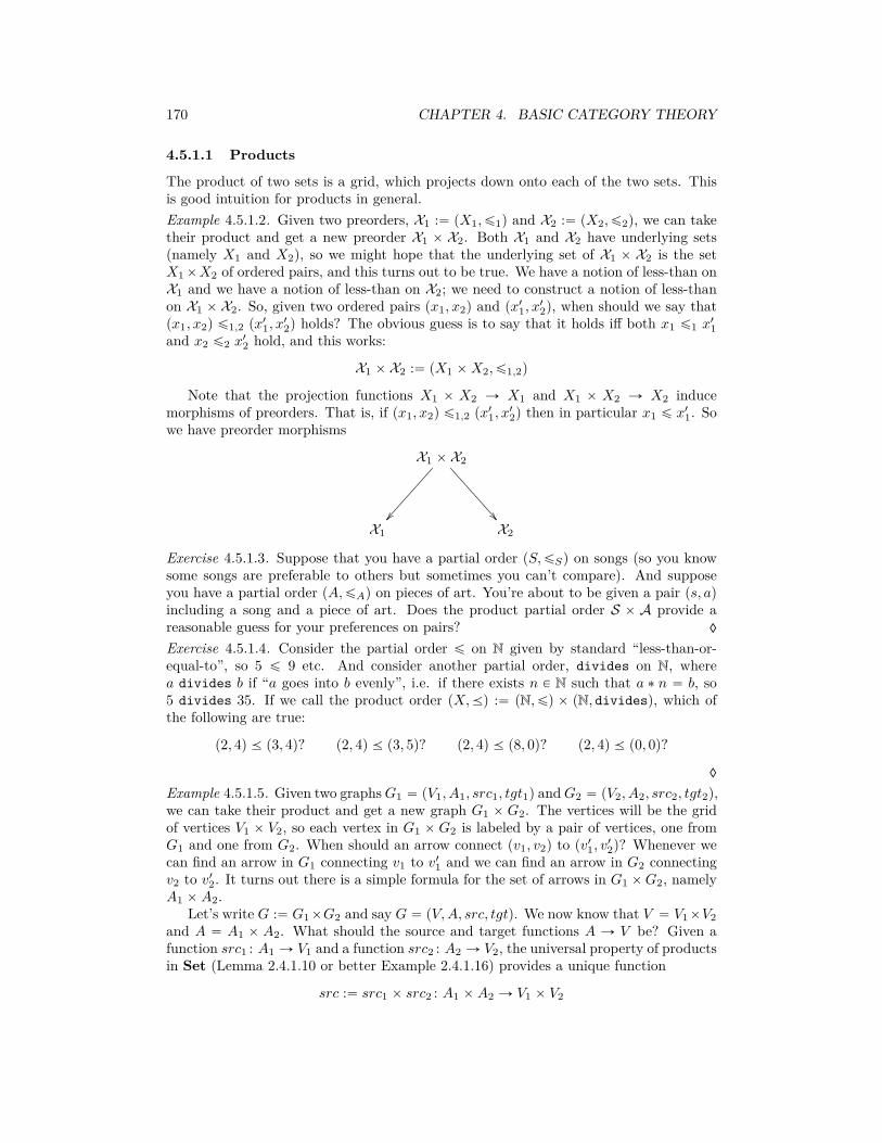
170 CHAPTER 4. BASIC CATEGORY THEORY
4.5.1.1 Products
The product of two sets is a grid, which projects down onto each of the two sets. Thisis good intuition for products in general.Example 4.5.1.2. Given two preorders, X1 :“ pX1,ď1q and X2 :“ pX2,ď2q, we can taketheir product and get a new preorder X1 ˆ X2. Both X1 and X2 have underlying sets(namely X1 and X2), so we might hope that the underlying set of X1 ˆ X2 is the setX1ˆX2 of ordered pairs, and this turns out to be true. We have a notion of less-than onX1 and we have a notion of less-than on X2; we need to construct a notion of less-thanon X1 ˆ X2. So, given two ordered pairs px1, x2q and px11, x12q, when should we say thatpx1, x2q ď1,2 px
11, x
12q holds? The obvious guess is to say that it holds iff both x1 ď1 x
11
and x2 ď2 x12 hold, and this works:
X1 ˆ X2 :“ pX1 ˆX2,ď1,2q
Note that the projection functions X1 ˆ X2 Ñ X1 and X1 ˆ X2 Ñ X2 inducemorphisms of preorders. That is, if px1, x2q ď1,2 px
11, x
12q then in particular x1 ď x11. So
we have preorder morphisms
X1 ˆ X2
�� ��X1 X2
Exercise 4.5.1.3. Suppose that you have a partial order pS,ďSq on songs (so you knowsome songs are preferable to others but sometimes you can’t compare). And supposeyou have a partial order pA,ďAq on pieces of art. You’re about to be given a pair ps, aqincluding a song and a piece of art. Does the product partial order S ˆ A provide areasonable guess for your preferences on pairs? ♦
Exercise 4.5.1.4. Consider the partial order ď on N given by standard “less-than-or-equal-to”, so 5 ď 9 etc. And consider another partial order, divides on N, wherea divides b if “a goes into b evenly”, i.e. if there exists n P N such that a ˚ n “ b, so5 divides 35. If we call the product order pX,ĺq :“ pN,ďq ˆ pN, dividesq, which ofthe following are true:
p2, 4q ĺ p3, 4q? p2, 4q ĺ p3, 5q? p2, 4q ĺ p8, 0q? p2, 4q ĺ p0, 0q?
♦
Example 4.5.1.5. Given two graphsG1 “ pV1, A1, src1, tgt1q andG2 “ pV2, A2, src2, tgt2q,we can take their product and get a new graph G1 ˆ G2. The vertices will be the gridof vertices V1 ˆ V2, so each vertex in G1 ˆG2 is labeled by a pair of vertices, one fromG1 and one from G2. When should an arrow connect pv1, v2q to pv11, v12q? Whenever wecan find an arrow in G1 connecting v1 to v11 and we can find an arrow in G2 connectingv2 to v12. It turns out there is a simple formula for the set of arrows in G1 ˆG2, namelyA1 ˆA2.
Let’s write G :“ G1ˆG2 and say G “ pV,A, src, tgtq. We now know that V “ V1ˆV2and A “ A1 ˆ A2. What should the source and target functions A Ñ V be? Given afunction src1 : A1 Ñ V1 and a function src2 : A2 Ñ V2, the universal property of productsin Set (Lemma 2.4.1.10 or better Example 2.4.1.16) provides a unique function
src :“ src1 ˆ src2 : A1 ˆA2 Ñ V1 ˆ V2

4.5. LIMITS AND COLIMITS 171
Namely the source of arrow pa1, a2q will be the vertex psrc1pa1q, src2pa2qq. Similarly wehave a ready-made choice of target function tgt “ tgt1 ˆ tgt2. We have now defined theproduct graph.
Here’s a concrete example. Let I and J be as drawn below:
I :“
v‚
f��w‚
g
��h
��x‚
J :“ q‚
i // r‚
j
s‚
k
__` // t‚
Arrow pIq
ID src tgtf v w
g w x
h w x
Vertex pIq
IDv
w
x
Arrow pJq
ID src tgti q r
j r s
k s r
` s t
Vertex pJq
IDq
r
s
t
The product IˆJ drawn below has, as expected 3˚4 “ 12 vertices and 3˚4 “ 12 arrows:
I ˆ J :“
pv,qq‚
pf,iq
!!
pv,rq‚
!!
pv,sq‚
}}
pv,tq‚
pw,qq‚
��%%
pw,rq‚
��%%
pw,sq‚
yy�� ��
%%
pw,tq‚
px,qq‚
px,rq‚
px,sq‚
px,tq‚
Arrow pI ˆ Jq
ID src tgtpf, iq pv, qq pw, rq
pf, jq pv, rq pw, sq
pf, kq pv, sq pw, rq
pf, `q pv, sq pw, tq
pg, iq pw, qq px, rq
pg, jq pw, rq px, sq
pg, kq pw, sq px, rq
pg, `q pw, sq px, tq
ph, iq pw, qq px, rq
ph, jq pw, rq px, sq
ph, kq pw, sq px, rq
ph, `q pw, sq px, tq
Vertex pI ˆ Jq
IDpv, qq
pv, rq
pv, sq
pv, tq
pw, qq
pw, rq
pw, sq
pw, tq
px, qq
px, rq
px, sq
px, tq
Here is the most important thing to notice. Look at the Arrow table for I ˆ J ,and for each ordered pair, look only at the second entry in all three columns; you willsee something that matches with the Arrow table for J . Do the same for I, and againyou’ll see a perfect match. These “matchings” are readily-visible graph homomorphismsI ˆ J Ñ I and I ˆ J Ñ J in Grph.
Exercise 4.5.1.6. Let r1s “ 0‚fÝÝÑ
1‚ be the linear order graph of length 1 and let P “
Pathspr1sq be its paths-graph, as in Example 4.1.2.22 (so P should have three arrowsand two vertices). Draw the graph P ˆ P . ♦
Exercise 4.5.1.7. Recall from Example 3.5.2.9 that a discrete dynamical system (DDS)is a set s together with a function f : sÑ s. By now it should be clear that if
Loop :“s‚
f��

172 CHAPTER 4. BASIC CATEGORY THEORY
is the loop schema, then a DDS is simply an instance (a functor) I : Loop Ñ Set. Wehave not yet discussed products of DDS’s, but perhaps you can guess how they shouldwork. For example, consider the instances I, J : LoopÑ Set tabulated below:
s (I)ID fA CB CC C
s (J)ID fx yy xz z
a.) Make a guess and tabulate I ˆ J . Then draw it.23
b.) Recall the notion of natural transformations between functors (see Example 4.3.3.5),which in the case of functors LoopÑ Set are the morphisms of instances. Do you seeclearly that there is a morphism of instances I ˆ J Ñ I and I ˆ J Ñ J? Just checkthat if you look only at the left-hand coordinates in your I ˆ J , you see somethingcompatible with I.
♦
In every case above, what’s most important to recognize is that there are projectionmaps IˆJ Ñ I and IˆJ Ñ J , and that the construction of IˆJ seems as straightforwardas possible, subject to having these projections. It is time to give the definition.
Definition 4.5.1.8. Let C be a category and let X,Y P ObpCq be objects. A span on Xand Y consists of three constituents pZ, p, qq, where Z P ObpCq is an object, and wherep : Z Ñ X and q : Z Ñ Y are morphisms in C.
Z
p
��
q
��X Y
A product of X and Y is a span X π1ÐÝ X ˆY
π2ÝÑ Y , 24 such that for any other span
XpÐÝ Z
qÝÑ Y there exists a unique morphism tp,q : Z Ñ X ˆ Y such that the diagram
below commutes:X ˆ Y
π1
��
π2
��X Y
Z
p
\\
q
BBtp,q
OO
Remark 4.5.1.9. Definition 4.5.1.8 endows the product of two objects with somethingknown as a universal property. It says that a product of two objects X and Y maps to
23The result is not necessarily inspiring, but at least computing it is straightforward.24The names X ˆ Y and π1, π2 are not mathematically important, they are pedagogically suggestive.

4.5. LIMITS AND COLIMITS 173
those two objects, and serves as a gateway for all who do the same. “None shall mapto X and Y except through me!” This grandiose property is held by products in all thevarious categories we have discussed so far. It is what I meant when I said things like“XˆY maps to both X and Y and does so as straightforwardly as possible”. The grid ofdots obtained as the product of two sets has such a property, as was shown in Example2.4.1.11.Example 4.5.1.10. In Example 4.5.1.2 we discussed products of preorders. In this examplewe will discuss products in an individual preorder. That is, by Proposition 4.2.1.17, thereis a functor PrO Ñ Cat that realizes every preorder as a category. If P “ pP,ďq isa preorder, what are products in P? Given two objects a, b P ObpPq we first considerspans on a and b, i.e. aÐ z Ñ b. That would be some z such that z ď a and z ď b. Theproduct will be such a span a ě aˆ b ď b, but such that every other spanning object zis less than or equal to a ˆ b. In other words a ˆ b is as big as possible subject to thecondition of being less than a and less than b. This is precisely the meet of a and b (seeDefinition 3.4.2.1).Example 4.5.1.11. Note that the product of two objects in a category C may not exist.Let’s return to preorders to see this phenomenon.
Consider the set R2, and say that px1, y1q ď px2, y2q if there exists ` ě 1 such thatx1` “ x2 and y1` “ y2; in other words, point p is less than point q if, in order to travelfrom q to the origin along a straight line, one must pass through p along the way. 25
We have given a perfectly good partial order, but p :“ p1, 0q and q :“ p0, 1q do nothave a product. Indeed, it would have to be a non-zero point that was on the sameline-through-the origin as p and the same line-through-the-origin as q, of which there arenone.Example 4.5.1.12. Note that there can be more than one product of two objects in acategory C, but that any two choices will be canonically isomorphic. Let’s return oncemore to preorders to see this phenomenon.
Consider the set R2 and say that px1, y1q ď px2, y2q if x21 ` y2
1 ď x22 ` y2
2 , in otherwords if the former is on a smaller 0-circle (by which I mean “circle centered at theorigin”) than the latter is.
For any two points p, q there will be lots of points that serve as products: anythingon the smaller of their two 0-circles will suffice. Given any two points a, b on this smallercircle, we will have a unique isomorphism a – b because a ď b and b ď a and allmorphisms are unique in a preorder.Exercise 4.5.1.13. Consider the preorder P of cards in a deck, shown in Example 3.4.1.3;it is not the entire story of cards in a deck, but take it to be so. In other words, be likea computer and take what’s there at face value. Consider the preorder P as a category(by way of the functor PrO Ñ Cat).
a.) For each of the following pairs, what is their product in P (if it exists)?
pa diamondqˆ pa heartq ? pa queenqˆ pa black cardq ?pa cardqˆ pa red cardq ? pa face cardqˆ pa black cardq ?
b.) How would these answers differ if P was completed to the “whole story” partial orderclassifying cards in a deck?
♦
25Note that p0, 0q is not related to anything else.

174 CHAPTER 4. BASIC CATEGORY THEORY
Exercise 4.5.1.14. Let X be a set, and consider it as a discrete category. Given twoobjects x, y P ObpXq, under what conditions will there exist a product xˆ y? ♦
Exercise 4.5.1.15. Let f : R Ñ R be a function, like you would see in 6th grade (maybefpxq “ x` 7). A typical thing to do is to graph f as a curve running through the planeR2 :“ Rˆ R. This curve can be understood as a function F : RÑ R2.
a.) Given some x P R, what are the coordinates of F pxq P R2?
b.) Obtain F : RÑ R2 using the universal property given in Definition 4.5.1.8.
♦
Exercise 4.5.1.16. Consider the preorder pN, dividesq, discussed in Exercise 4.5.1.4,where e.g. 5 ď 15 but 5 ę 6.
a.) What is the product of 9 and 12 in this category?
b.) Is there a standard name for products in this category?
♦
Example 4.5.1.17. All products exist in the category Cat. Given two categories C andD, there is a product category C ˆ D. We have ObpC ˆ Dq “ ObpCq ˆ ObpDq and forany two objects pc, dq and pc1, d1q, we have
HomCˆDppc, dq, pc1, d1qq “ HomCpc, c
1q ˆHomCpd, d1q.
The composition formula is “obvious”.Let r1s P ObpCatq denote the linear order category of length 1, drawn
r1s :“ 0‚
f // 1‚
As a schema it has one arrow, but as a category it has three morphisms. So we expectr1sˆr1s to have 9 morphisms, and that’s true. In fact, r1sˆr1s looks like a commutativesquare:
p0,0q‚
id0ˆf //
fˆid0
��
p0,1q‚
fˆid1
��p1,0q‚
id1ˆf// p1,1q‚
(4.17)
We see only four morphisms here, but there are also four identities and one morphismp0, 0q Ñ p1, 1q given by composition of either direction. It is a minor miracle that thecategorical product somehow “knows” that this square should commute; however, this isnot the mere preference of man but instead the dictate of God! By which I mean, thisfollows rigorously from the definitions we already gave of Cat and products.
4.5.1.18 Coproducts
The coproduct of two sets is their disjoint union, which includes non-overlapping copiesof each of the two sets. This is good intuition for coproducts in general.
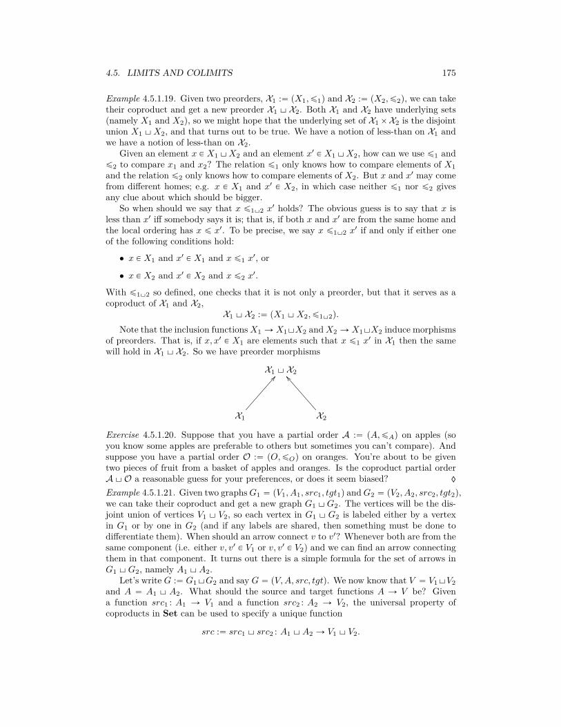
4.5. LIMITS AND COLIMITS 175
Example 4.5.1.19. Given two preorders, X1 :“ pX1,ď1q and X2 :“ pX2,ď2q, we can taketheir coproduct and get a new preorder X1 \ X2. Both X1 and X2 have underlying sets(namely X1 and X2), so we might hope that the underlying set of X1ˆX2 is the disjointunion X1 \X2, and that turns out to be true. We have a notion of less-than on X1 andwe have a notion of less-than on X2.
Given an element x P X1\X2 and an element x1 P X1\X2, how can we use ď1 andď2 to compare x1 and x2? The relation ď1 only knows how to compare elements of X1and the relation ď2 only knows how to compare elements of X2. But x and x1 may comefrom different homes; e.g. x P X1 and x1 P X2, in which case neither ď1 nor ď2 givesany clue about which should be bigger.
So when should we say that x ď1\2 x1 holds? The obvious guess is to say that x is
less than x1 iff somebody says it is; that is, if both x and x1 are from the same home andthe local ordering has x ď x1. To be precise, we say x ď1\2 x
1 if and only if either oneof the following conditions hold:
• x P X1 and x1 P X1 and x ď1 x1, or
• x P X2 and x1 P X2 and x ď2 x1.
With ď1\2 so defined, one checks that it is not only a preorder, but that it serves as acoproduct of X1 and X2,
X1 \ X2 :“ pX1 \X2,ď1\2q.
Note that the inclusion functionsX1 Ñ X1\X2 andX2 Ñ X1\X2 induce morphismsof preorders. That is, if x, x1 P X1 are elements such that x ď1 x
1 in X1 then the samewill hold in X1 \ X2. So we have preorder morphisms
X1 \ X2
X1
AA
X2
]]
Exercise 4.5.1.20. Suppose that you have a partial order A :“ pA,ďAq on apples (soyou know some apples are preferable to others but sometimes you can’t compare). Andsuppose you have a partial order O :“ pO,ďOq on oranges. You’re about to be giventwo pieces of fruit from a basket of apples and oranges. Is the coproduct partial orderA\O a reasonable guess for your preferences, or does it seem biased? ♦
Example 4.5.1.21. Given two graphsG1 “ pV1, A1, src1, tgt1q andG2 “ pV2, A2, src2, tgt2q,we can take their coproduct and get a new graph G1 \G2. The vertices will be the dis-joint union of vertices V1 \ V2, so each vertex in G1 \ G2 is labeled either by a vertexin G1 or by one in G2 (and if any labels are shared, then something must be done todifferentiate them). When should an arrow connect v to v1? Whenever both are from thesame component (i.e. either v, v1 P V1 or v, v1 P V2) and we can find an arrow connectingthem in that component. It turns out there is a simple formula for the set of arrows inG1 \G2, namely A1 \A2.
Let’s write G :“ G1\G2 and say G “ pV,A, src, tgtq. We now know that V “ V1\V2and A “ A1 \ A2. What should the source and target functions A Ñ V be? Givena function src1 : A1 Ñ V1 and a function src2 : A2 Ñ V2, the universal property ofcoproducts in Set can be used to specify a unique function
src :“ src1 \ src2 : A1 \A2 Ñ V1 \ V2.
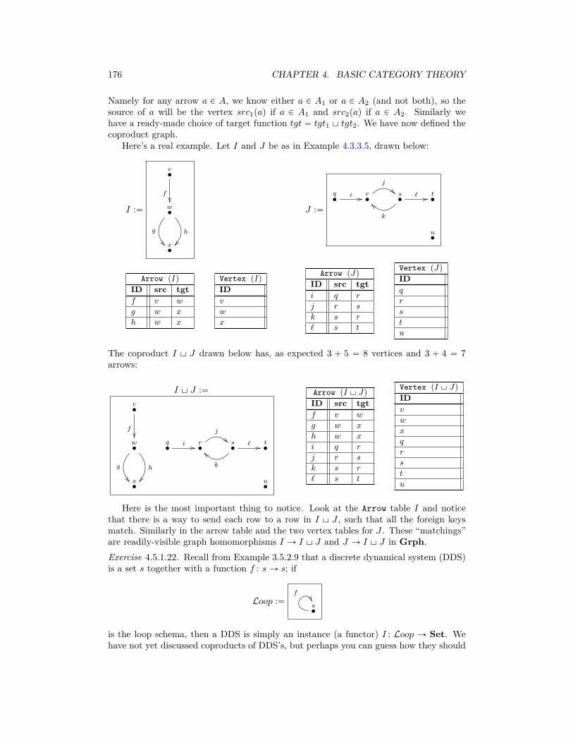
176 CHAPTER 4. BASIC CATEGORY THEORY
Namely for any arrow a P A, we know either a P A1 or a P A2 (and not both), so thesource of a will be the vertex src1paq if a P A1 and src2paq if a P A2. Similarly wehave a ready-made choice of target function tgt “ tgt1 \ tgt2. We have now defined thecoproduct graph.
Here’s a real example. Let I and J be as in Example 4.3.3.5, drawn below:
I :“
v‚
f��w‚
g
��h
��x‚
J :“
q‚
i // r‚
j
s‚
k
__` // t‚
u‚
Arrow pIq
ID src tgtf v w
g w x
h w x
Vertex pIq
IDv
w
x
Arrow pJq
ID src tgti q r
j r s
k s r
` s t
Vertex pJq
IDq
r
s
t
u
The coproduct I \ J drawn below has, as expected 3 ` 5 “ 8 vertices and 3 ` 4 “ 7arrows:
I \ J :“v‚
f��w‚
g
��h
��
q‚
i // r‚
j
s‚
k
__` // t‚
x‚
u‚
Arrow pI \ Jq
ID src tgtf v w
g w x
h w x
i q r
j r s
k s r
` s t
Vertex pI \ Jq
IDv
w
x
q
r
s
t
u
Here is the most important thing to notice. Look at the Arrow table I and noticethat there is a way to send each row to a row in I \ J , such that all the foreign keysmatch. Similarly in the arrow table and the two vertex tables for J . These “matchings”are readily-visible graph homomorphisms I Ñ I \ J and J Ñ I \ J in Grph.Exercise 4.5.1.22. Recall from Example 3.5.2.9 that a discrete dynamical system (DDS)is a set s together with a function f : sÑ s; if
Loop :“s‚
f��
is the loop schema, then a DDS is simply an instance (a functor) I : Loop Ñ Set. Wehave not yet discussed coproducts of DDS’s, but perhaps you can guess how they should

4.5. LIMITS AND COLIMITS 177
work. For example, consider the instances I, J : LoopÑ Set tabulated below:
s (I)ID fA CB CC C
s (J)ID fx yy xz z
Make a guess and tabulate I \ J . Then draw it. ♦
In every case above (preorders, graphs, DDSs), what’s most important to recognizeis that there are inclusion maps I Ñ I \ J and J Ñ I \ J , and that the construction ofI \ J seems as straightforward as possible, subject to having these inclusions. It is timeto give the definition.
Definition 4.5.1.23. Let C be a category and let X,Y P ObpCq be objects. A cospanon X and Y consists of three constituents pZ, i, jq, where Z P ObpCq is an object, andwhere i : X Ñ Z and j : Y Ñ Z are morphisms in C.
Z
X
i
EE
Y
j
XX
A coproduct of X and Y is a cospan Xι1ÝÑ X \ Y
ι2ÐÝ Y , 26 such that for any other
cospan XiÝÑ Z
jÐÝ Y there exists a unique morphism si,j : X \ Y Ñ Z such that the
diagram below commutes:X \ Y
si,j
��
X
ι1
BB
i
��
Y
ι2
\\
j
��Z
Remark 4.5.1.24. Definition 4.5.1.8 endows the coproduct of two objects with a universalproperty. It says that a coproduct of two objects X and Y receives maps from those twoobjects, and serves as a gateway for all who do the same. “None shall receive maps fromX and Y except through me!” This grandiose property is held by all the coproducts wehave discussed so far. It is what I meant when I said things like “X \ Y receives mapsfrom both X and Y and does so as straightforwardly as possible”. The disjoint unionof dots obtained as the coproduct of two sets has such a property, as can be seen bythinking about Example 2.4.2.5.Example 4.5.1.25. By Proposition 4.2.1.17, there is a functor PrO Ñ Cat that realizesevery preorder as a category. If P “ pP,ďq is a preorder, what are coproducts in P?Given two objects a, b P ObpPq we first consider cospans on a and b, i.e. a Ñ z Ð b.
26The names X \ Y and ι1, ι2 are not mathematically important, they are pedagogically suggestive.

178 CHAPTER 4. BASIC CATEGORY THEORY
A cospan of a and b is any z such that a ď z and b ď z. The coproduct will be such acospan a ď a \ b ě b, but such that every other cospanning object z is greater than orequal to a \ b. In other words a \ b is as small as possible subject to the condition ofbeing bigger than a and bigger than b. This is precisely the join of a and b (see Definition3.4.2.1).
Just as for products, the coproduct of two objects in a category C may not exist, or itmay not be unique. The non-uniqueness is much less “bad” because given two candidatecoproducts, they will be canonically isomorphic. They may not be equal, but they areisomorphic. But coproducts might not exist at all in certain categories. We will explorethat a bit below.Example 4.5.1.26. Consider the set R2 and partial order from Example 4.5.1.11 wherepx1, y1q ď px2, y2q if there exists ` ě 1 such that x1` “ x2 and y1` “ y2. Again thepoints p :“ p1, 0q and q :“ p0, 1q do not have a coproduct. Indeed, it would have tobe a non-zero point that was on the same line-through-the origin as p and the sameline-through-the-origin as q, of which there are none.Exercise 4.5.1.27. Consider the preorder P of cards in a deck, shown in Example 3.4.1.3;it is not the entire story of cards in a deck, but take it to be so. In other words, be like acomputer and take what’s there at face value. Consider the preorder P as a category (byway of the functor PrO Ñ Cat). For each of the following pairs, what is their coproductin P (if it exists)?
a.) pa diamondq\pa heartq ? pa queenq\pa black cardq ?
pa cardq\pa red cardq ? pa face cardq\pa black cardq ?
b.) How would these answers differ if P was completed to the “whole story” partial orderclassifying cards in a deck?
♦
Exercise 4.5.1.28. Let X be a set, and consider it as a discrete category. Given twoobjects x, y P ObpXq, under what conditions will there exist a coproduct x\ y? ♦
Exercise 4.5.1.29. Consider the preorder pN, dividesq, discussed in Exercise 4.5.1.4,where e.g. 5 ď 15 but 5 ę 6.
a.) What is the coproduct of 9 and 12 in that category?
b.) Is there a standard name for coproducts in that category?
♦
4.5.2 Diagrams in a categoryWe have been drawing diagrams since the beginning of the book. What is it that wehave been drawing pictures of? The answer is that we have been drawing functors.
Definition 4.5.2.1. Let C and I be categories. 27 An I-shaped diagram in C is simplya functor d : I Ñ C. In this case I is called the indexing category for the diagram.
27In fact, the indexing category I is usually assumed to be small in the sense of Remark 4.1.1.2,meaning that its collection of objects is a set.

4.5. LIMITS AND COLIMITS 179
Suppose given an indexing category I and an I-shaped diagram X : I Ñ C. Onedraws this as follows. For each object in q P I, draw a dot labeled by Xpqq; if severalobjects in I point to the same object in C, then several dots will be labeled the same way.Draw the images of morphisms f : q Ñ q1 in I by drawing arrows between dots Xpqqand Xpq1q, and label each arrow by the image morphism Xpfq in C. Again, if severalmorphisms in I are sent to the same morphism in C, then several arrows will be labeledthe same way. One can abbreviate this process by not drawing every morphism in I, solong as every morphism in I is represented by a unique path in C, i.e. as long as thedrawing is sufficiently unambiguous as a depiction of X : I Ñ C.
Example 4.5.2.2. Consider the commutative diagram in Set drawn below:
N`1 //
˚2��
N
˚2��
N`2// Z
(4.18)
This is the drawing of a functor d : r1s ˆ r1s Ñ Set (see Example 4.5.1.17). Withnotation for the objects and morphisms of r1sˆ r1s as shown in Diagram (4.17), we havedp0, 0q “ dp0, 1q “ dp1, 0q “ N and dp1, 1q “ Z (for some reason..) and dpid0, fq : NÑ Ngiven by n ÞÑ n` 1, etc.
The fact that d is a functor means it must respect composition formulas, which impliesthat Diagram (4.18) commutes. Recall from Section 2.2 that not all diagrams one candraw will commute; one must specify that a given diagram commutes if he or she wishesto communicate this fact. But then how is a non-commuting diagram to be understoodas a functor?
Let G P ObpGrphq denote the following graph
p0,0q‚
f //
h ��
p0,1q‚
g��
p1,0q‚
i// p1,1q‚
Recall the free category functor F : Grph Ñ Cat from Example 4.1.2.30. The freecategory F pGq P ObpCatq on G looks almost like r1s ˆ r1s except that since rf, gs is adifferent path in G than is rh, is, they become different morphisms in F pGq. A functorF pGq Ñ Set might be drawn the same way that (4.18) is, but it would be a diagramthat would not be said to commute.
We call r1s ˆ r1s the commutative square indexing category. 28
Exercise 4.5.2.3. Consider r2s, the linear order category of length 2.
a.) Is r2s the appropriate indexing category for commutative triangles?
b.) If not, what is?
♦
28We might call what is here denoted by F pGq the noncommutative square indexing category.
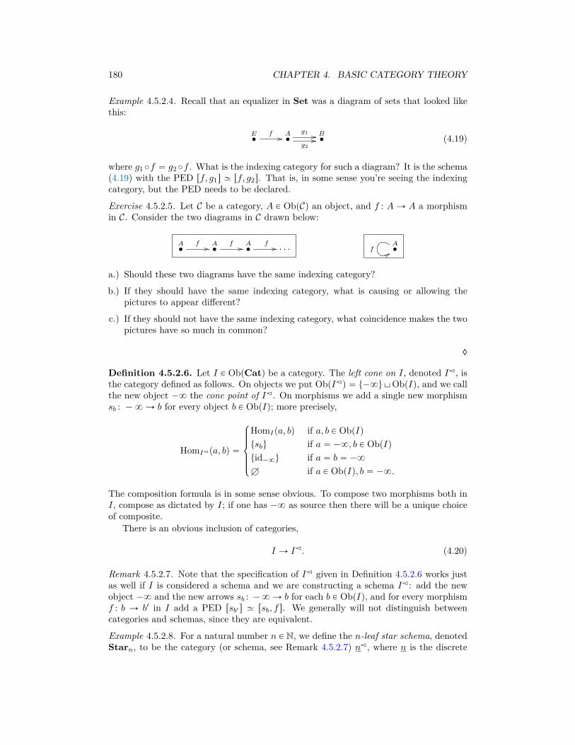
180 CHAPTER 4. BASIC CATEGORY THEORY
Example 4.5.2.4. Recall that an equalizer in Set was a diagram of sets that looked likethis:
E‚
f // A‚g1 //g2//B‚ (4.19)
where g1 ˝f “ g2 ˝f . What is the indexing category for such a diagram? It is the schema(4.19) with the PED rf, g1s » rf, g2s. That is, in some sense you’re seeing the indexingcategory, but the PED needs to be declared.
Exercise 4.5.2.5. Let C be a category, A P ObpCq an object, and f : AÑ A a morphismin C. Consider the two diagrams in C drawn below:
A‚
f // A‚f // A‚
f // ¨ ¨ ¨A‚f 99
a.) Should these two diagrams have the same indexing category?
b.) If they should have the same indexing category, what is causing or allowing thepictures to appear different?
c.) If they should not have the same indexing category, what coincidence makes the twopictures have so much in common?
♦
Definition 4.5.2.6. Let I P ObpCatq be a category. The left cone on I, denoted IŸ, isthe category defined as follows. On objects we put ObpIŸq “ t´8u\ObpIq, and we callthe new object ´8 the cone point of IŸ. On morphisms we add a single new morphismsb : ´8 Ñ b for every object b P ObpIq; more precisely,
HomIŸpa, bq “
$
’
’
’
&
’
’
’
%
HomIpa, bq if a, b P ObpIqtsbu if a “ ´8, b P ObpIqtid´8u if a “ b “ ´8
H if a P ObpIq, b “ ´8.
The composition formula is in some sense obvious. To compose two morphisms both inI, compose as dictated by I; if one has ´8 as source then there will be a unique choiceof composite.
There is an obvious inclusion of categories,
I Ñ IŸ. (4.20)
Remark 4.5.2.7. Note that the specification of IŸ given in Definition 4.5.2.6 works justas well if I is considered a schema and we are constructing a schema IŸ: add the newobject ´8 and the new arrows sb : ´8 Ñ b for each b P ObpIq, and for every morphismf : b Ñ b1 in I add a PED rsb1s » rsb, f s. We generally will not distinguish betweencategories and schemas, since they are equivalent.
Example 4.5.2.8. For a natural number n P N, we define the n-leaf star schema, denotedStarn, to be the category (or schema, see Remark 4.5.2.7) nŸ, where n is the discrete

4.5. LIMITS AND COLIMITS 181
category on n objects. Below we draw Star0,Star1,Star2, and Star3.
Star0
´8‚
Star1
´8‚
s1
��1‚
Star2
´8‚
s1
��
s2
��1‚
2‚
Star3
´8‚
s1
��
s2
��
s3
��1‚
2‚
3‚
Exercise 4.5.2.9. Let C0 :“ 0 denote the empty category and for any natural numbern P N, let Cn`1 “ pCnqŸ. Draw C4. ♦
Exercise 4.5.2.10. Let C be the graph indexing schema as in (4.7). What is CŸ and howdoes it compare to (4.19)? ♦
Definition 4.5.2.11. Let I P ObpCatq be a category. The right cone on I, denoted IŹ,is the category defined as follows. On objects we put ObpIŹq “ ObpIq\t8u, and we callthe new object 8 the cone point of IŹ. On morphisms we add a single new morphismtb : bÑ8 for every object b P ObpIq; more precisely,
HomIŹpa, bq “
$
’
’
’
&
’
’
’
%
HomIpa, bq if a, b P ObpIqttbu if a P ObpIq, b “ 8tid8u if a “ b “ 8
H if a “ 8, b P ObpIq.
The composition formula is in some sense obvious. To compose two morphisms both inI, compose as dictated by I; if one has 8 as target then there will be a unique choice ofcomposite.
There is an obvious inclusion of categories I Ñ IŹ.Exercise 4.5.2.12. Let C be the category p2ŸqŹ, where 2 is the discrete category on twoobjects. Then C is somehow square-shaped, but what category is it exactly? Lookingat Example 4.5.2.2, is C the commutative diagram indexing category r1s ˆ r1s, is it thenon-commutative diagram indexing category F pGq, or is it something else? ♦
4.5.3 Limits and colimits in a categoryLet C be a category, let I be an indexing category (which just means that I is a categorythat we’re about to use as the indexing category for a diagram), and let D : I Ñ C anI-shaped diagram (which just means a functor). It is in relation to this setup that wecan discuss the limit or colimit. In general the limit of a diagram D : I Ñ C will be a IŸshaped diagram limD : IŸ Ñ C. In the case of products I “ 2 and IŸ “ Star2 lookslike a span (see Example 4.5.2.8). But out of all the IŸ-shaped diagrams, which is thelimit of D? Answer: the one with the universal “gateway” property, see Remark 4.5.1.9.
4.5.3.1 Universal objects
Definition 4.5.3.2. Let C be a category. An object a P ObpCq is called initial if, forall objects c P ObpCq there exists a unique morphism a Ñ c, i.e. |HomCpa, cq| “ 1. Anobject z P ObpCq is called terminal if, for all objects c P ObpCq there is exists a uniquemorphism cÑ z, i.e. |HomCpc, zq| “ 1.

182 CHAPTER 4. BASIC CATEGORY THEORY
An object in a category is called universal if it is either initial or terminal, but werarely use that term in practice, preferring to be specific about whether the object isinitial or terminal. The word final is synonymous with the word terminal, but we’ll tryto constantly use terminal.
Colimits will end up being defined as initial things of a certain sort, and limits willend up being defined as terminal things of a certain sort. But we will get to that inSection 4.5.3.15.Warning 4.5.3.3. A category C may have more than one initial object; similarly a categoryC may have more than one terminal object. We will see in Example 4.5.3.5 that any setwith one element, e.g. t˚u or t,u, is a terminal object in Set. These terminal sets havethe same number of elements, but they are not the exact-same set; two sets having thesame cardinality means precisely that there exists an isomorphism between them.
In fact, Proposition 4.5.3.4 below shows that in any category C, any two terminalobjects in C are isomorphic (similarly, any two initial objects in C are isomorphic).While there are many isomorphisms in Set between t1, 2, 3u and ta, b, cu, there is onlyone isomorphism between t˚u and ,. This is always the case for universal objects: thereis a unique isomorphism between any two terminal (respectively initial) objects in anycategory.
As a result, people often speak of the initial object in C or the terminal object in C,as though there was only one. “It’s unique up to unique ismorphism!” is the justificationfor this use of the so-called definite article the rather than the indefinite article a. Thisis not a very misleading way of speaking, because just like the president today does notcontain exactly the same atoms as the president yesterday, the difference is unimportant.But we still mention this as a warning: if C has a terminal object, we may speak of it asthough it were unique, calling it the terminal object, and similarly for initial objects.
We will use the definite article throughout this document, e.g. in Example 4.5.3.5we will discuss the initial object in Set and the terminal object in Set. This is commonthroughout mathematical literature as well.
Proposition 4.5.3.4. Let C be a category and let a1, a2 P ObpCq both be initial objects.Then there is a unique isomorphism a1
–ÝÑ a2. (Similarly, for any two terminal objects
in C there is a unique isomorphism between them.)
Proof. Suppose a1 and a2 are initial. Since a1 is initial there is a unique morphismf : a1 Ñ a2; there is also a unique morphism a1 Ñ a1, which must be ida1 . Since a2 isinitial there is a unique morphism g : a2 Ñ a1; there is also a unique morphism a2 Ñ a2,which must be ida2 . So g ˝ f “ ida1 and f ˝ g “ ida2 , which means that f is the desired(unique) isomorphism.
The proof for terminal objects is appropriately “dual”.�
Example 4.5.3.5. The initial object in Set is the set a for which there is always one wayto map from a to anything else. Given c P ObpSetq there is exactly one function HÑ c,because there are no choices to be made, so the empty set H is the initial object in Set.
The terminal object in Set is the set z for which there is always one way to map toz from anything else. Given c P ObpSetq there is exactly one function c Ñ t,u, wheret,u is any set with one element, because there are no choices to be made: everything inc must be sent to the single element in t,u. There are lots of terminal objects in Set,and they are all isomorphic to 1.

4.5. LIMITS AND COLIMITS 183
Example 4.5.3.6. The initial object in Grph is the graph a for which there is always oneway to map from a to anything else. Given c P ObpGrphq, there is exactly one functionHÑ c, where H P Grph is the empty graph; so H is the initial object.
The terminal object in Grph is more interesting. It is Loop, the graph with onevertex and one arrow. In fact there are infinitely many terminal objects in Grph, butall of them are isomorphic to Loop.Exercise 4.5.3.7. Let X be a set, let PpXq be the set of subsets of X (see Definition2.7.4.9). We can regard PpXq as a preorder under inclusion of subsets (see for exampleSection 3.4.2). And we can regard preorders as categories using a functor PrO Ñ Cat(see Proposition 4.2.1.17).
a.) What is the initial object in PpXq?
b.) What is the terminal object in PpXq?
♦
Example 4.5.3.8. The initial object in the category Mon of monoids is the trivial monoid,1. For any monoid M , a morphism of monoids 1 Ñ M is a functor between 1-objectcategories and these are determined by where they send morphisms. Since 1 has onlythe identity morphism and functors must preserve identities, there is no choice involvedin finding a monoid morphism 1 ÑM .
Similarly, the terminal object in Mon is also the trivial monoid, 1. For any monoidM , a morphism of monoids M Ñ 1 sends everything to the identity; there is no choice.Exercise 4.5.3.9.
a.) What is the initial object in Grp, the category of groups?
b.) What is the terminal object in Grp?
♦
Example 4.5.3.10. Recall the preorder Prop of logical propositions from Section 4.2.4.1.The initial object is a proposition that implies all others. It turns out that “FALSE” issuch a proposition. The proposition “FALSE” is like “1 ‰ 1”; in logical formalism it canbe shown that if “FALSE” is true then everything is true.
The terminal object in Prop is a proposition that is implied by all others. It turnsout that “TRUE” is such a proposition. In logical formalism, everything implies that“TRUE” is true.Example 4.5.3.11. The discrete category 2 has no initial object and no terminal ob-ject. The reason is that it has two objects 1, 2, but no maps from one to the other, soHom2p1, 2q “ Hom2p2, 1q “ H.Exercise 4.5.3.12. Recall the divides preorder from Exercise 4.5.1.4, where 5 divides 15.
a.) Considering this preorder as a category, does it have an initial object?
b.) Does it have a terminal object?
♦
Exercise 4.5.3.13. Let M “ pListpta, buq, r s, ` q denote the free monoid on ta, bu (seeDefinition 3.1.1.15), considered as a category (via Theorem 4.2.1.3).
a.) Does it have an initial object?

184 CHAPTER 4. BASIC CATEGORY THEORY
b.) Does it have a terminal object?
c.) Which monoids have initial (respectively terminal) objects?
♦
Exercise 4.5.3.14. Let S be a set and consider the indiscrete category KS P ObpCatq onobjects S (see Example 4.3.4.3).
a.) For what S does KS have an initial object?
b.) For what S does KS have a terminal object?
♦
4.5.3.15 Examples of limits
Let C be a category and let X,Y P ObpCq be objects. Definition 4.5.1.8 defines a productof X and Y to be a span X π1
ÐÝ XˆYπ2ÝÑ Y such that for every other span X p
ÐÝ ZqÝÑ Y
there exists a unique morphism Z Ñ X ˆY making the triangles commute. It turns outthat we can enunciate this in our newly formed language of universal objects by sayingthat the span X
π1ÐÝ X ˆ Y
π2ÝÑ Y is itself a terminal object in the category of spans
on X and Y . Phrasing the definition of products in this way will be generalizable todefining arbitrary limits.Construction 4.5.3.16 (Products). Let C be a category and let X1, X2 be objects. We canconsider this setup as a diagram X : 2 Ñ C, where Xp1q “ X1 and Xp2q “ X2. Considerthe category 2Ÿ “ Star2, which is drawn in Example 4.5.2.8; the inclusion i : 2 Ñ 2Ÿ, asin (4.20); and the category of functors Funp2Ÿ, Cq. The objects in Funp2Ÿ, Cq are spansin C and the morphisms are natural transformations between them. Given a functorS : 2Ÿ Ñ C we can compose with i : 2 Ñ 2Ÿ to get a functor 2 Ñ C. We want that to beX.
2 X //
i
��
C
2ŸS
??
So we are ready to define the category of spans on X1 and X2.Define the category of spans on X, denoted C{X , to be the category whose objects
and morphisms are as follows:
ObpC{Xq “ tS : 2Ÿ Ñ C | S ˝ i “ Xu (4.21)HomC{X pS, S
1q “ tα : S Ñ S1 | α ˝ i “ idXu.
The product of X1 and X2 was defined in Definition 4.5.1.8; we can now recast X1ˆX2as the terminal object in C{X .
To bring this down to earth, an object in C{X can be pictured as a diagram in C ofthe following form:
Z
p
��
q
��X1 X2

4.5. LIMITS AND COLIMITS 185
In other words, the objects of C{X are spans, each of which we might write in-line as
X1pÐÝ Z
qÝÑ X2. A morphism in C{X from object X1
pÐÝ Z
qÝÑ X2 to object X1
p1
ÐÝ Z 1q1
ÝÑ
X2 consists of a morphism ` : Z Ñ Z 1, such that p1 ˝ ` “ p and q1 ˝ ` “ q. So the set ofsuch morphisms in C{X are all the `’s that make the right-hand diagram commute: 29
HomC{X
¨
˚
˚
˝
Z
p
��q
��X1 X2
,
Z 1
p1
��q1
��X1 X2
˛
‹
‹
‚
“
$
’
’
’
’
’
’
’
’
’
’
’
’
&
’
’
’
’
’
’
’
’
’
’
’
’
%
Z
p
��
q
��`
��
X1 X2
Z 1
p1
YY
q1
EE
,
/
/
/
/
/
/
/
/
/
/
/
/
.
/
/
/
/
/
/
/
/
/
/
/
/
-
(4.22)
Each object in C{X is a span on X1 and X2, and each morphism in C{X is a “morphismof cone points in C making everything in sight commute”. The terminal object in C{X isthe product of X1 and X2; see Definition 4.5.1.8.
It may be strange to have a category in which the objects are spans in anothercategory. But once you admit this possibility, the notion of morphism between spansis totally sensible. Or if it isn’t, then stare at (4.22) for 30 seconds and say to yourself“When in Rome..!” These are the aqueducts of category theory, and they work wonders.
Example 4.5.3.17. Consider the arbitrary 6-object category C drawn below, in which the
29To be completely pedantic, according to (4.21), the morphisms in C{X should be drawn like this:
HomC{X
¨
˚
˚
˚
˚
˝
Z
p
��q
��X1 X2
,
Z 1
p1
��q1
��X1 X2
˛
‹
‹
‹
‹
‚
“
$
’
’
’
’
’
’
’
’
’
’
’
’
’
’
’
’
’
’
’
’
’
’
’
&
’
’
’
’
’
’
’
’
’
’
’
’
’
’
’
’
’
’
’
’
’
’
’
%
Z
p
��
q
��
α´8
��
X1
α1
X2
α2
X1 X2
Z 1
p1
YY
q1
EE
,
/
/
/
/
/
/
/
/
/
/
/
/
/
/
/
/
/
/
/
/
/
/
/
.
/
/
/
/
/
/
/
/
/
/
/
/
/
/
/
/
/
/
/
/
/
/
/
-
But this is going a bit overboard. The point is, the set HomC{X is the set of morphisms serving the roleof α´8 : Z Ñ Z1.

186 CHAPTER 4. BASIC CATEGORY THEORY
three diagrams that can commute do:
C :“
X1‚
A‚
a
22
B‚
foo
X b1
@@
b2
��
C‚
X
X
c1
^^
c2
��
g // D‚
d1
ll
d2rrX2
‚
Let X : 2 Ñ C be given by Xp1q “ X1 and Xp2q “ X2. Then the category of spans onX might be drawn
C{X – pB,b1,b2q‚
pC,c1,c2q‚
g // pD,d1,d2q‚
4.5.3.18 Definition of limit
Definition 4.5.3.19. Let C be a category, let I be a category; let IŸ be the left cone onI, and let i : I Ñ IŸ be the inclusion. Suppose that X : I Ñ C is an I-shaped diagramin C. The slice category of C over X denoted C{X is the category whose objects andmorphisms are as follows:
ObpC{Xq “ tS : IŸ Ñ C | S ˝ i “ Xu
HomC{X pS, S1q “ tα : S Ñ S1 | α ˝ i “ idXu.
A limit of X, denoted limI X or limX, is a terminal object in C{X .
Pullbacks The relevant indexing category for pullbacks is the cospan, I “ 2Ź drawnas to the left below:
I
0‚
��
1‚
��2‚
X : I Ñ CX0‚
��
X1‚
��X2‚
30
A I-shaped diagram in C is a functor X : I Ñ C, which we might draw as to the rightabove (e.g. X0 P ObpCq).
30We use a dash box here because we’re not drawing the whole category but merely a diagram existinginside C.
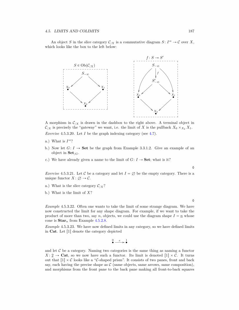
4.5. LIMITS AND COLIMITS 187
An object S in the slice category C{X is a commutative diagram S : IŸ Ñ C over X,which looks like the box to the left below:
S P ObpC{Xq
S´8
!!}}X0‚
X1‚
~~X2‚
f : S Ñ S1
S´8
��
f
��S1´8
~~X0‚
X1‚
~~X2‚
A morphism in C{X is drawn in the dashbox to the right above. A terminal object inC{X is precisely the “gateway” we want, i.e. the limit of X is the pullback X0 ˆX2 X1.Exercise 4.5.3.20. Let I be the graph indexing category (see 4.7).
a.) What is IŸ?
b.) Now let G : I Ñ Set be the graph from Example 3.3.1.2. Give an example of anobject in Set{G.
c.) We have already given a name to the limit of G : I Ñ Set; what is it?
♦
Exercise 4.5.3.21. Let C be a category and let I “ H be the empty category. There is aunique functor X : HÑ C.
a.) What is the slice category C{X?
b.) What is the limit of X?
♦
Example 4.5.3.22. Often one wants to take the limit of some strange diagram. We havenow constructed the limit for any shape diagram. For example, if we want to take theproduct of more than two, say n, objects, we could use the diagram shape I “ n whosecone is Starn from Example 4.5.2.8.Example 4.5.3.23. We have now defined limits in any category, so we have defined limitsin Cat. Let r1s denote the category depicted
0‚
e // 1‚
and let C be a category. Naming two categories is the same thing as naming a functorX : 2 Ñ Cat, so we now have such a functor. Its limit is denoted r1s ˆ C. It turnsout that r1s ˆ C looks like a “C-shaped prism”. It consists of two panes, front and backsay, each having the precise shape as C (same objects, same arrows, same composition),and morphisms from the front pane to the back pane making all front-to-back squares

188 CHAPTER 4. BASIC CATEGORY THEORY
commute. For example, if C looked was the category generated by the schema to the leftbelow, then C ˆ r1s would be the category generated by the schema to the right below:
A‚
f //
g
��
B‚
h
��C‚
D‚
A1‚
f1 //
g1 ��
B1‚
h1
��
A0‚
Ae
@@
f0 //
g0
��
B0‚
Be
@@
h0
��
C1‚
D1‚
C0‚
Ce
@@
D0‚
De
@@
It turns out that a natural transformation α : F Ñ G between functors F,G : C Ñ Dis the same thing as a functor C ˆ r1s Ñ D such that the front pane is sent via Fand the back pane is sent via G. The components are captured by the front-to-backmorphisms, and the naturality is captured by the commutativity of the front-to-backsquares in C ˆ r1s.
Remark 4.5.3.24. Recall in Section 2.7.6.6 we described relative sets. In fact, Definition2.7.6.7 basically defines a category of relative sets over any fixed set B. Let 1 denote thediscrete category on one object, and note that providing a functor 1 Ñ Set is the sameas simply providing a set, so consider B : 1 Ñ Set. Then the slice category Set{B , asdefined in Definition 4.5.3.19 is precisely the category of relative sets over B: it has thesame objects and morphisms as was described in Definition 2.7.6.7.
4.5.3.25 Definition of colimit
The definition of colimits is appropriately “dual” to the definition of limits. Insteadof looking at left cones, we look at right cones; instead of being interested in terminalobjects, we are interested in initial objects.
Definition 4.5.3.26. Let C be a category, let I be a category; let IŹ be the right coneon I, and let i : I Ñ IŹ be the inclusion. Suppose that X : I Ñ C is an I-shaped diagramin C. The coslice category of C over X denoted CX{ is the category whose objects andmorphisms are as follows:
ObpCX{q “ tS : IŹ Ñ C | S ˝ i “ Xu
HomCX{pS, S1q “ tα : S Ñ S1 | α ˝ i “ idXu.
A colimit of X, denoted colimI X or colimX, is an initial object in CX{.

4.5. LIMITS AND COLIMITS 189
Pushouts The relevant indexing category for pushouts is the span, I “ 2Ÿ drawn asto the left below:
I
1‚
2‚
0‚
\\ BB
X : I Ñ CX1‚
X2‚
X0‚
^^ @@
An I-shaped diagram in C is a functor X : I Ñ C, which we might draw as to the rightabove (e.g. X0 P ObpCq).
An object S in the coslice category CX{ is a commutative diagram S : IŹ Ñ C overX, which looks like the box to the left below:
S P ObpCX{q
S8
X1‚
>>
X2‚
``
X0‚
__ ??
f : S Ñ S1
S18
S8
f
OO
X1‚
>>
<<
X2‚
``
aa
X0‚
??__
A morphism in CX{ is drawn in the dashbox to the right above. An initial object in CX{is precisely the “gateway” we want; i.e. the colimit of X is the pushout, X1 \X0 X2.
Exercise 4.5.3.27. Let I be the graph indexing category (see 4.7).
a.) What is IŹ?
b.) Now let G : I Ñ Set be the graph from Example 3.3.1.2. Give an example of anobject in SetG{.
c.) We have already given a name to the colimit of G : I Ñ Set; what is it?
♦
Exercise 4.5.3.28. Let C be a category and let I “ H be the empty category. There is aunique functor X : HÑ C.
a.) What is the coslice category CX{?
b.) What is the colimit of X (assuming it exists)?
♦

190 CHAPTER 4. BASIC CATEGORY THEORY
Example 4.5.3.29 (Cone as colimit). We have now defined colimits in any category, so wehave defined colimits in Cat. Let C be a category and recall from Example 4.5.3.23 thecategory C ˆ r1s. The inclusion of the front pane is a functor i0 : C Ñ C ˆ r1s (similarly,the inclusion of the back pane is a functor i1 : C Ñ C ˆ r1s). Finally let t : C Ñ 1 be theunique functor to the terminal category (see Exercise 4.1.2.37). We now have a diagramin Cat of the form
C i0 //
t
��
C ˆ r1s
1
The colimit (i.e. the pushout) of this diagram in Cat slurps down the entire front paneof C ˆ r1s to a point, and the resulting category is isomorphic to CŸ. Figure 4.23 is adrawing of this phenomenon.

4.5. LIMITS AND COLIMITS 191
C :“A0‚ //
��
B0‚
��C0‚
D0‚
i0 //
C ˆ r1s
A1‚ //
��
B1‚
��
A0‚
@@
//
��
B0‚
@@
��
C1‚
D1‚
C0‚
@@
D0‚
@@
t
�� ��
´8‚
1
//
A1‚ //
��
B1‚
��
´8‚
??
��
__
��C1‚
D1‚
CŸ – pC ˆ r1sq \C 1
Figure 4.23: Let C be the category drawn in the upper left corner. The left cone CŸ onC is obtained as a pushout in Cat. We first make a prism C ˆ r1s, and then identify thefront pane with a point.
(Similarly, the pushout of the analogous diagram for i1 would give CŹ.)
Example 4.5.3.30. Consider the category Top of topological spaces. The (hollow) circleis a topological space which people often denote S1 (for “1-dimensional sphere”). Thefilled-in circle, also called a 2-dimensional disk, is denoted D2. The inclusion of the circleinto the disk is continuous so we have a morphism in Top of the form i : S1 Ñ D2. Theterminal object in Top is the one-point space t,u, and so there is a unique morphismt : S1 Ñ t,u. The pushout of the diagram D2 i
ÐÝ S1 tÝÑ t,u is isomorphic to the
2-dimensional sphere (the exterior of a tennis ball), S2. The reason is that we haveslurped the entire bounding circle to a point, and the category of topological spaces hasthe right morphisms to ensure that the resulting space really is a sphere.

192 CHAPTER 4. BASIC CATEGORY THEORY
Application 4.5.3.31. Consider the symmetric graphGn consisting of a chain of n vertices,
1‚
2‚ ¨ ¨ ¨
n‚
Think of this as modeling a subway line. There are n-many graph homomorphismsG1 Ñ Gn given by the various vertices. One can create transit maps using colimits. Forexample, the colimit of the diagram to the left is the symmetric graph drawn to the rightbelow.
colim
¨
˚
˚
˚
˚
˚
˚
˚
˚
˚
˚
˝
G14 //
4��
G7 G16oo
1��
G5 G3
G1
2
OO
3// G7 G1
2
OO
5oo
˛
‹
‹
‹
‹
‹
‹
‹
‹
‹
‹
‚
can be drawn
‚5
1‚
2‚
3‚
4‚4
5‚
6‚1
7‚
‚3
1‚
2‚
3‚2
4‚
5‚2
6‚
7‚
‚1 ‚3
♦♦
4.6 Other notions in CatIn this section we discuss some leftover notions about categories. For example in Section4.6.1 we explain a kind of duality for categories, in which arrows are flipped. For examplereversing the order in a preorder is an example of this duality, as is the similarity betweenlimits and colimits. In Section 4.6.2 we discuss the so-called Grothendieck constructionwhich in some sense graphs functors, and we show that it is useful for transformingdatabases into the kind of format (RDF) used in scraping data off webpages. We definea general construction for creating categories in Section 4.6.4. Finally, in Section 4.6.5we show that precisely the same arithmetic statements that held for sets in Section 2.7.3hold for categories.
4.6.1 Opposite categoriesPeople used to discuss two different kinds of functors between categories: the so-calledcovariant functors and the so-called contravariant functors. Covariant functors arewhat we have been calling functors. The reader may have come across the idea ofcontravariance when considering Exercise 4.2.3.2.31 There we saw that a continuousmapping of topological spaces f : X Ñ Y does not induce a morphism of orders ontheir open sets OpenpXq Ñ OpenpY q; that is not required by the notion of continuity.Instead, a morphism of topological spaces f : X Ñ Y induces a morphism of ordersOpenpY q Ñ OpenpXq, going backwards. So we do not have a functor Top Ñ PrOin this way, but it’s quite close. One used to say that Open is a contravariant functorTop Ñ PrO.
31Similarly, see Exercise 4.2.4.4.

4.6. OTHER NOTIONS IN CAT 193
As important and common as contravariance is, people found that keeping track ofwhich functors were covariant and which were contravariant was a big hassle. Luck-ily, there is a simple work-around, which simplifies everything: the notion of oppositecategories.
Definition 4.6.1.1. Let C be a category. The opposite category of C, denoted Cop, hasthe same objects as C, i.e. ObpCopq “ ObpCq, and for any two objects c, c1, one defines
HomCoppc, c1q :“ HomCpc1, cq.
Example 4.6.1.2. If n P N is a natural number and n the corresponding discrete category,then nop “ n. Recall the span category I “ 2Ÿ from Definition 4.5.1.8. Its opposite isthe cospan category Iop “ 2Ź, from Definition 4.5.1.23.Exercise 4.6.1.3. Let C be the category from Example 4.5.3.17. Draw Cop. ♦
Lemma 4.6.1.4. Let C and D be categories. One has pCopqop “ C. Also we haveFunpC,Dq – FunpCop,Dopq. This implies that a functor Cop Ñ D can be identified witha functor C Ñ Dop.
Proof. This follows straightforwardly from the definitions.�
Exercise 4.6.1.5. In Exercises 4.2.3.2, 4.2.4.3, and 4.2.4.4 there were questions aboutwhether a certain function ObpCq Ñ ObpDq extended to a functor C Ñ D. In each case,see if the proposed function would extend to a “contravariant functor” i.e. to a functorCop Ñ D. ♦
Example 4.6.1.6 (Simplicial sets). Recall from Example 4.3.4.4 the category ∆ of linearorders rns. For example, r1s is the linear order 0 ď 1 and r2s is the linear order 0 ď 1 ď 2.Both r1s and r2s are objects of ∆. There are 6 morphisms from r1s to r2s, which wecould denote
Hom∆pr1s, r2sq “ tp0, 0q, p0, 1q, p0, 2q, p1, 1q, p1, 2q, p2, 2qu.
It may seem strange, but the category ∆op turns out to be quite useful in algebraictopology. It is the indexing category for a combinatorial approach to the homotopytheory of spaces. That is, we can represent something like the category of spaces andcontinuous maps using the functor category sSet :“ Funp∆op,Setq, which is called thecategory of simplicial sets.
This may seem very complicated compared to something we did earlier, namely sim-plicial complexes. But simplicial sets have excellent formal properties that simplicialcomplexes do not. We will not go further with this here, but through the work of DanKan, Andre Joyal, Jacob Lurie, and many others, simplicial sets have allowed categorytheory to pierce deeply into the realm of topology and vice versa.
4.6.2 Grothendieck constructionLet C be a database schema (or category) and let J : C Ñ Set be an instance. We havebeen drawing this in table form, but there is another standard way of laying out the datain J , called the resource descriptive framework or RDF. Developed for the web, RDF is auseful format when one does not have a schema in hand, e.g. when scraping information

194 CHAPTER 4. BASIC CATEGORY THEORY
off of a website, one does not know what schema will be best. In these cases, informationis stored in so-called RDF triples, which are of the form
xSubject, Predicate, Objecty
For example, one might see something like
Subject Predicate ObjectA01 occurredOn D13114A01 performedBy P44A01 actionDescription Told congress to raise debt ceilingD13114 hasYear 2013D13114 hasMonth JanuaryD13114 hasDay 14P44 FirstName BarackP44 LastName Obama
(4.24)
Category-theoretically, it is quite simple to convert a database instance J : C Ñ Setinto an RDF triple store. To do so, we use the Grothendieck construction, which is moreaptly named the category of elements construction, defined below.32
Definition 4.6.2.1. Let C be a category and let J : C Ñ Set be a functor. The categoryof elements of J , denoted
ş
C J , is defined as follows:
Obpw
C
Jq :“ tpC, xq | C P ObpCq, x P JpCqu.
Homş
C JppC, xq, pC 1, x1qq :“ tf : C Ñ C 1 | Jpfqpxq “ x1u.
There is a natural functor πJ :ş
C J ÝÑ C. It sends each object pC, xq P Obpş
C Jq tothe object C P ObpCq. And it sends each morphism f : pC, xq Ñ pC 1, x1q to the morphismf : C Ñ C 1. We call πJ the projection functor.
Example 4.6.2.2. Let A be a set, and consider it as a discrete category. We saw inExercise 4.3.3.4 that a functor S : A Ñ Set is the same thing as an A-indexed set, asdiscussed in Section 2.7.6.10. We will follow Definition 2.7.6.12 and for each a P A writeSa :“ Spaq.
What is the category of elements of a functor S : AÑ Set? The objects ofş
AS are
pairs pa, sq where a P A and s P Spaq. Since A has nothing but identity morphisms,ş
AS
has nothing but identity morphisms; i.e. it is the discrete category on a set. In fact thatset is the disjoint union w
A
S “ğ
aPA
Sa.
The functor πS :ş
AS Ñ A sends each element in Sa to the element a P A.
32Apparently, Alexander Grothendieck did not invent this construction, it was discussed prior toGrothendieck’s use of it, e.g. by Mac Lane. But more to the point, the term Grothendieck construction isnot grammatically suited in the sense that both the following are awkward in English: “the Grothendieckconstruction of J is ...” (awkward because J is not being constructed but used in a construction) and“the Grothendieck construct for J is...” (awkward because it just is). The term category of elements ismore descriptive and easier to use grammatically.

4.6. OTHER NOTIONS IN CAT 195
One can see this as a kind of histogram. For example, let A “ tBOS, NYC, LA, DCu andlet S : AÑ Set assign
SBOS “ tAbby, Bob, Casandrau,
SNYC “ H,
SLA “ tJohn, Jimu, andSDC “ tAbby, Carlau.
Then the category of elements of S would look like the (discrete) category at the top:
w
A
S “
pBOS,Abbyq‚
pBOS,Bobq‚
pLA,Johnq‚
pDC,Abbyq‚
pBOS,Casandraq‚
pLA,Jimq‚
pDC,Carlaq‚
(4.25)
πS
��
A “ BOS‚
NYC‚
LA‚
DC‚
We also see that the category of elements construction has converted an A-indexedset into a relative set over A, as in Definition 2.7.6.7.
The above example does not show at all how the Grothendieck construction trans-forms a database instance into an RDF triple store. The reason is that our databaseschema was A, a discrete category that specifies no connections between data (it simplycollects the data into bins). So lets examine a more interesting database schema andinstance. This is taken from [Sp2].Application 4.6.2.3. Consider the schema below, which we first encountered in Example3.5.2.1:
C :“
Employee manager worksIn » Employee worksInDepartment secretary worksIn » Department
Employee‚
worksIn //
manager��
first
~~
last
��
Department‚
secretaryoo
name
��FirstNameString
‚LastNameString
‚DepartmentNameString
‚
(4.26)

196 CHAPTER 4. BASIC CATEGORY THEORY
And consider the instance J : C Ñ Set, which we first encountered in (3.13) and (3.15)
EmployeeID first last manager worksIn101 David Hilbert 103 q10102 Bertrand Russell 102 x02103 Emmy Noether 103 q10
DepartmentID name secretaryq10 Sales 101x02 Production 102
FirstNameStringIDAlanBertrandCarlDavidEmmy
LastNameStringIDArdenHilbertJonesNoetherRussell
DepartmentNameStringIDMarketingProductionSales
The category of elements of J : C Ñ Set looks like this:
w
C
J “
101‚
first
��
last
,,
manager
AA
worksIn
((102‚
103‚
q10‚
x02‚
secretary
hh
name
}}
Alan‚
Hilbert‚
Production‚
Bertrand‚
Russell‚
Sales‚
David‚
Noether‚
Marketing‚
Emmy‚
Arden‚
Carl‚
Jones‚
πJ
��
(4.27)
C “
Employee‚
worksIn //
manager��
first
��
last
��
Department‚
secretaryoo
name
��FirstNameString‚
LastNameString‚
DepartmentNameString‚

4.6. OTHER NOTIONS IN CAT 197
In the above drawing (4.27) ofş
C J , we left out 10 arrows for ease of readability, forexample, we left out an arrow 102
‚first
ÝÝÝÝÝÝÑBertrand‚ .
For the punchline, how do we see the category of elementsş
C J as an RDF triplestore? For each arrow in
ş
C J , we take the triple consisting of the source vertex, thearrow name, and the target vertex. So our triple store would include triples such asx102 first Bertrandy and x101 manager 103y.
♦♦
Exercise 4.6.2.4. Come up with a schema and instance whose category of elements con-tains (at least) the data from (4.24). ♦
Slogan 4.6.2.5.
“ The Grothendieck construction takes structured, boxed-up data and flattensit by throwing it all into one big space. The projection functor is then taskedwith remembering which box each datum originally came from. ”
Exercise 4.6.2.6. Recall from Section 3.1.2.10 that a finite state machine is a free monoidpListpΣq, r s, ` q acting on a set X. Recall also that we can consider a monoid as acategory M with one object and a monoid action as a set-valued functor F : MÑ Set,(see Section 4.2.1.1). In the case of Figure 3.1 the monoid in question is Listpa, bq, whichcan be drawn as the schema
Na
9999
b
eeee
and the functor F : M Ñ Set is recorded in an action table in Example 3.1.3.1. Whatisş
M F? How does it relate to the picture in Figure 3.1? ♦
4.6.3 Full subcategoryDefinition 4.6.3.1. Let C be a category and let X Ď ObpCq be a set of objects in C.The full subcategory of C spanned by X is the category, which we denote by COb“X , withobjects ObpCOb“Xq :“ X and with morphisms HomCOb“X
px, x1q :“ HomCpx, x1q.
Example 4.6.3.2. The following are examples of full subcategories. We will name them inthe form “X inside of Y ”, and each time we mean that X and Y are names of categories,the category X can be considered as a subcategory of the category Y in some sense, andit is full. In other words, all morphisms in Y “count” as morphisms in X.
• Finite sets inside of sets, Fin Ď Set;
• Finite sets of the form n inside of Fin;
• Linear orders of the form rns inside of all finite linear orders, ∆ Ď FLin;
• Groups inside of monoids, Grp Ď Mon;
• Monoids inside of categories, Mon Ď Cat;
• Sets inside of graphs, Set Ď Grph;
• Partial orders (resp. linear orders) inside of PrO;

198 CHAPTER 4. BASIC CATEGORY THEORY
• Discrete categories (resp. indiscrete categories) inside of Cat;
Remark 4.6.3.3. A subcategory C Ď D is (up to isomorphism) just a functor i : C Ñ Dthat happens to be injective on objects and arrows. The subcategory is full if and onlyif i is a full functor in the sense of Definition 4.3.4.12.Example 4.6.3.4. Let C be a category, let X Ď ObpCq be a set of objects, and let COb“Xdenote the full subcategory of C spanned by X. We can realize this as a fiber productof categories. Indeed, recall that for any set, we can form the indiscrete category onthat set; see Example 4.3.4.3. In fact, we have a functor Ind : Set Ñ Cat. Thusour function X Ñ ObpCq can be converted into a functor between indiscrete categoriesIndpXq Ñ IndpObpCqq. There is also a functor C Ñ IndpObpCqq sending each object toitself. Then the full subcategory of C spanned by X is the fiber product of categories,
COb“X //
��
C
��IndpXq // IndpObpCqq
Exercise 4.6.3.5. Including all identities and all compositions, how many morphisms arethere in the full subcategory of Set spanned by the objects t0, 1, 2u? Write them out. ♦
4.6.4 Comma categoriesCategory theory includes a highly developed and interoperable catalogue of materialsand production techniques. One such is the comma category.
Definition 4.6.4.1. Let A,B, and C be categories and let F : A Ñ C and G : B Ñ Cbe functors. The comma category of C morphisms from F to G, denoted pF ÓC Gq orsimply pF Ó Gq, is the category with objects
ObpF Ó Gq “ tpa, b, fq | a P ObpAq, b P ObpBq, f : F paq Ñ Gpbq in Cu
and for any two objects pa, b, fq and pa1, b1, f 1q the set HompFÓGqppa, b, fq, pa1, b1, f 1qq ofmorphisms pa, b, fq ÝÑ pa1, b1, f 1q is
tpq, rq | q : aÑ a1 in A, r : bÑ b1 in B, such that f 1 ˝ F pqq “ Gprq ˝ fu.
In pictures,
HompFÓGqppa, b, fq, pa1, b1, f 1qq :“
$
’
’
’
’
’
&
’
’
’
’
’
%
a
q
��
F paq
X
f //
F pqq
��
Gpbq
Gprq
��
b
r
��a1 F pa1q
f 1// Gpb1q b1
,
/
/
/
/
/
.
/
/
/
/
/
-
We refer to the diagram A FÝÑ C G
ÐÝ B (in Cat) as the setup for the comma categorypF Ó Gq.
There is a canonical functor pF Ó Gq Ñ A called left projecton, sending pa, b, fq to a,and a canonical functor pF Ó Gq Ñ B called right projection, sending pa, b, fq to b.

4.6. OTHER NOTIONS IN CAT 199
A setup A FÝÑ C G
ÐÝ B is reversable; i.e. we can flip it to obtain B GÝÑ C F
ÐÝ A.However, note that pF Ó Gq is different than (i.e. almost never equivalent to) pG Ó F q,unless every arrow in C is an isomorphism.
Slogan 4.6.4.2.
“ When two categories A,B can be interpreted in a common setting C, thecomma category integrates them by recording how to move from A to Binside C. ”
Example 4.6.4.3. Let C be a category and I : C Ñ Set a functor. In this example weshow that the comma category construction captures the notion of taking the categoryof elements
ş
C I; see Definition 4.6.2.1.Consider the set 1, the category Discp1q, and the functor F : Discp1q Ñ Set sending
the unique object to the set 1. We use the comma category setup 1 FÝÝÝÑ Set I
ÐÝÝÝ C.There is an isomorphism of categories
ż
CI – pF Ó Iq.
Indeed, an object in pF Ó Iq is a triple pa, b, fq where a P Obp1q, b P ObpCq, andf : F paq Ñ Ipbq is a morphism in Set. There is only one object in 1, so this reduces toa pair pb, fq where b P ObpCq and f : t,u Ñ Ipbq. The set of functions t,u Ñ Ipbq isisomorphic to Ipbq, as we saw in Exercise 2.1.2.14. So we have reduced ObpF Ó Iq to theset of pairs pb, xq where b P ObpCq and x P Ipbq; this is Obp
ş
C Iq. Because there is onlyone function 1 Ñ 1, a morphism pb, xq Ñ pb1, x1q in pF Ó Iq boils down to a morphismr : bÑ b1 such that the diagram
1 x // Ipbq
Iprq
��1
x1// Ipb1q
commutes. But such diagrams are in one-to-one correspondence with the diagramsneeded for morphisms in
ş
C I.Exercise 4.6.4.4. Let C be a category and let c, c1 P ObpCq be objects. Consider themas functors c, c1 : 1 Ñ C, and consider the setup 1 c
ÝÝÝÑ C c1ÐÝÝÝ 1. What is the comma
category pc Ó c1q? ♦
4.6.5 Arithmetic of categoriesIn Section 2.7.3, we summarized some of the properties of products, coproducts, andexponentials for sets, attempting to show that they lined up precisely with familiararithmetic properties of natural numbers. Astoundingly, we can do the same for cate-gories.
In the following proposition, we denote the coproduct of two categories A and B bythe notation A` B rather than A\ B. We also denote the functor category FunpA,Bqby BA. Finally, we use 0 and 1 to refer to the discrete category on 0 and on 1 object,respectively.
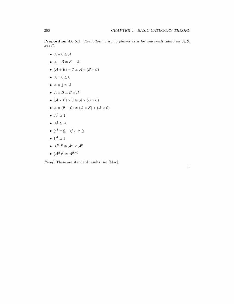
200 CHAPTER 4. BASIC CATEGORY THEORY
Proposition 4.6.5.1. The following isomorphisms exist for any small categories A,B,and C.
• A` 0 – A
• A` B – B `A
• pA` Bq ` C – A` pB ` Cq
• Aˆ 0 – 0
• Aˆ 1 – A
• Aˆ B – B ˆA
• pAˆ Bq ˆ C – Aˆ pB ˆ Cq
• Aˆ pB ` Cq – pAˆ Bq ` pAˆ Cq
• A0 – 1
• A1 – A
• 0A – 0, if A ‰ 0
• 1A – 1
• AB`C – AB ˆAC
• pABqC – ABˆC
Proof. These are standard results; see [Mac].�

MIT OpenCourseWarehttp://ocw.mit.edu
18.S996�Category Theory for ScientistSpring 2013
For information about citing these materials or our Terms of Use, visit: http://ocw.mit.edu/terms.