18.330 Lecture Notes: Modulation: Wireless Communication ...homerreid.dyndns.org/teaching/18.330/Notes/Modulation.pdf · 18.330 Lecture Notes: Modulation: Wireless Communication and

18.330 Lecture Notes:

Modulation: Wireless Communication and

Lock-in Amplifiers

Homer Reid

April 3, 2014

Contents

1 Overview 2

2 Analog modulation 32.1 Amplitude modulation (AM) . . . . . . . . . . . . . . . . . . . . 32.2 Phase and frequency modulation (PM and FM) . . . . . . . . . . 7

3 Digital modulation 93.1 OOK . . . . . . . . . . . . . . . . . . . . . . . . . . . . . . . . . . 93.2 BPSK, QPSK, MPSK . . . . . . . . . . . . . . . . . . . . . . . . 93.3 QAM . . . . . . . . . . . . . . . . . . . . . . . . . . . . . . . . . 103.4 Spectral efficiency . . . . . . . . . . . . . . . . . . . . . . . . . . 10

4 Multiplex methods 134.1 The cocktail party . . . . . . . . . . . . . . . . . . . . . . . . . . 144.2 How CDMA works . . . . . . . . . . . . . . . . . . . . . . . . . . 14

5 Lock-in amplifiers 155.1 How lock-in amplifiers work . . . . . . . . . . . . . . . . . . . . . 15

1

18.330 Lecture Notes 2

1 Overview

Consider a bandlimited baseband signal fBB(t) with bandwidth ∆ω.1 A goodexample to have in mind is music: think of fBB(t) as the time-dependent voltageV (t) output from your MP3 player to your headphones or speakers. In this case,fBB(t) is a bandlimited baseband signal with a bandwidth ∆ω ≈ 2π · 20 kHz.(The superscript “BB” stands for “baseband.”)

For various reasons, it may be desirable to convert the signal fBB(t) intoa new signal fM(t) whose frequency spectrum has the same bandwidth as theoriginal signal fBB(t), but is centered around a nonzero frequency called thecarrier frequency, ωcarrier. The process of translating frequencies in this way iscalled modulation. (The “M” superscript stands for “modulated.” In some caseswe will also refer to fM as f transmitted to indicate that it is the signal that iseventually transmitted over a wired or wireless communication channel.)

Modulation is ubiquitous throughout all fields of science and engineeringand forms the essential cornerstone of modern communications technologies. Italso furnishes an example of a highly practical and relevant real-world problemwhich would be essentially impossible to tackle without the ideas and techniquesof Fourier analysis.

The purpose of these short notes is to introduce some of the basic techniquesof modulation and compare their spectral efficiencies. We will focus primarilyon communication technologies, but we will also briefly discuss lock-in detectionas an important application of modulation techniques in experimental science.

1A bandlimited signal with bandwidth ∆ω is a function f(t) whose Fourier transform f(ω)is zero for frequencies ω outside an interval of width ∆ω. A baseband signal is a signal whosefrequency spectrum is centered at ω = 0.


2 Analog modulation

2.1 Amplitude modulation (AM)

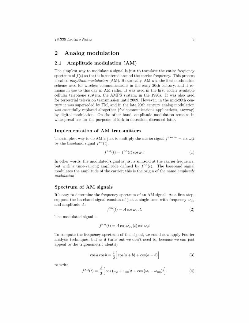
The simplest way to modulate a signal is just to translate the entire frequencyspectrum of f(t) so that it is centered around the carrier frequency. This processis called amplitude modulation (AM). Historically, AM was the first modulationscheme used for wireless communications in the early 20th century, and it re-mains in use to this day in AM radio. It was used in the first widely availablecellular telephone system, the AMPS system, in the 1980s. It was also usedfor terrestrial television transmission until 2009. However, in the mid-20th cen-tury it was superseded by FM, and in the late 20th century analog modulationwas essentially replaced altogether (for communications applications, anyway)by digital modulation. On the other hand, amplitude modulation remains inwidespread use for the purposes of lock-in detection, discussed later.

Implementation of AM transmitters

The simplest way to do AM is just to multiply the carrier signal f carrier = cosωctby the baseband signal fBB(t):

fAM(t) = fBB(t) cosωct (1)

In other words, the modulated signal is just a sinusoid at the carrier frequency,but with a time-varying amplitude defined by fBB(t). The baseband signalmodulates the amplitude of the carrier; this is the origin of the name amplitudemodulation.

Spectrum of AM signals

It’s easy to determine the frequency spectrum of an AM signal. As a first step,suppose the baseband signal consists of just a single tone with frequency ωBB

and amplitude A:fBB(t) = A cosωBBt. (2)

The modulated signal is

fAM(t) = A cosωBB(t) cosωct

To compute the frequency spectrum of this signal, we could now apply Fourieranalysis techniques, but as it turns out we don’t need to, because we can justappeal to the trigonometric identity

cos a cos b =1

2

[cos(a+ b) + cos(a− b)

](3)

to write

fAM(t) =A

2

[cos(ωc + ωBB)t+ cos

(ωc − ωBB)t

]. (4)


This is a frequency spectrum with nonvanishing contributions from just twofrequencies, namely, ωc ± ωBB.

Of course, usually our baseband signal will be more interesting than just thesingle tone (2). However, any baseband signal can be decomposed into a sumof single tones through the magic of Fourier analysis. For the time being, let’ssuppose fBB is a periodic baseband signal that is an even function of time; thenits Fourier decomposition looks something like

fBB(t) =∑ωn

fBB(ωn) cosωnt.

Each term in this sum contributes two terms to the frequency spectrum of theoutput signal just as in equation (4):

fAM(t) =∑ωn

fBB(ωn)

2

[cos(ωc + ωn

)t+ cos

(ωc − ωn

)t]. (5)

Equation (5) describes a frequency spectrum consisting of two copies of thefrequency spectrum of fBB(t), with the two copies mirrored about the carrierfrequency. In particular, the bandwidth of the transmit signal is twice thebndwidth of the baseband signal. Each mirrored copy is called a sideband, andthis type of amplitude modulation is known as double-sideband modulation.

Figures 1 and 2 show the baseband, carrier, and modulated signals in thetime and frequency domains.


-0.5

0

0.5

1

1.5

0 0.5 1 1.5 2-0.5

0

0.5

1

1.5

y

t

-1.5

-1

-0.5

0

0.5

1

1.5

0 0.5 1 1.5 2-1.5

-1

-0.5

0

0.5

1

1.5

y

t

-1.5

-1

-0.5

0

0.5

1

1.5

0 0.5 1 1.5 2-1.5

-1

-0.5

0

0.5

1

1.5

y

t

Figure 1: Amplitude modulation in the time domain.


1

y

t

1

y

t

1

y

t

Figure 2: Amplitude modulation in the frequency domain. The baseband signalhas some frequency spectrum that is nonzero up to a maximum frequency ωmax.The carrier signal has a frequency spectrum that is concentrated at a singlepoint. The modulated signal has a frequency spectrum consisting of two copies(two “sidebands”) of the baseband frequency spectrum mirrored about the car-rier frequency. The modulated signal has bandwidth 2ωmax. Single-sidebandmodulation would produce a similar signal but with only one of the two side-bands present.


Single-sideband AM

As we noted above, the frequency spectrum of a naıve AM signal contains tworedundant copies of the information we are trying to transmit. This means thatthe transmit signal actually has twice as much bandwidth as it nominally needsto have to transmit the requisite information.

It is possible to circumvent this redundancy by use of a technique known assingle-sideband modulation. This is based on the following modified version ofthe trig identity (3):

cos a cos b− sin a sin b = cos(a+ b).

To see how single-sideband modulation works in practice, suppose again thatour baseband signal consist of the single tone

fBB(t) = A cosωBBt.

What we do is to form the π/2-shifted-version of this signal:

fBB

π/2(t) = A sinωBBt.

Then we multiply fBB(t) by the original carrier signal cosωct, and we multi-ply the π/2 shifted baseband signal by the π/2 shifted carrier signal, and wesubtract:

fSSAM(t) = fBB(t) cosωct− fBB

π/2 sinωct

For the case of the single-tone baseband signal, the transmit signal now containsonly the single tone ωc + ωBB; the lower-sideband tone at ωc − ωBB has beensupressed. More generally, if fBB(t) contains a spectrum of frequencies, thetransmitted signal will contain only one copy of this spectrum, not the tworedundant copies we found above.

However, for baseband signals that are more complicated than a single tone,forming the π/2 shifted version is expensive: we have to Fourier-decomposethe signal into constituent sinusoids and then apply a π/2 phase shift to eachsinusoid. In practice this requires fairly sophisticated digital signal processingtechniques, and is not commonly used for wireless AM communications.

2.2 Phase and frequency modulation (PM and FM)

One drawback of amplitude modulation is that all the information is in theamplitude of the received signal, which makes that signal susceptible to noisecontamination. This will be evident to anyone who has ever experienced annoy-ing hissing and ringing sounds from an AM radio.

An alternative technique is modulate the phase and/or frequency of thecarrier instead of its amplitude. The former option is called phase modulation(PM), The latter option is called frequency modulation (FM), and collectivelythey are sometimes known as angle modulation. In the time domain, the signals


take the form

fPM = cos[ωct+ αfBB(t)

]fFM = cos

[ωct+ α

∫ t

0

fBB(t′) dt]

where α is a parameter known as the modulation index that determines thefractional extent to which we allow the carrier phase and frequency to be tweakedby the baseband signal.

-1.5

-1

-0.5

0

0.5

1

1.5

0 0.5 1 1.5 2-1.5

-1

-0.5

0

0.5

1

1.5

y

t

Figure 3: An example of a FM signal in the time domain. Note that theamplitude is fixed, but the instantaneous frequency varies.

Angle modulation techniques have the advantage that all the information iscontained in the zero crossings of the signal, which make them less sensitive tonoise contamination. However, this advantage comes at a cost: for the samebaseband signal, PM and FM signals occupy significantly more bandwidth thanAM signals. A real-world demonstration of this fact may be found in the spacingof AM and FM radio stations: AM stations are typically spaced about 10 kHzapart from one another, while FM stations are typically spaced around 500 kHzfrom each other, even though they are nominally transmitting baseband signalsof the same bandwidth (music and talk, which occupies up to around 20 kHz).


3 Digital modulation

AM and FM are techniques for transmitting analog signals. We may also wantto transmit a digital signal – that is, a sequence of 0s and 1s. There are manyways to do this, of which we will consider just a few.

3.1 OOK

The simplest form of digital modulation is known as on-off keying (OOK).In this scheme, the carrier is turned on for the duration of each 1 bit in thebitstream, and turned off for the duration of each 0 bit.

0 1 2 3 4 5t

Figure 4: OOK transmit signal.

3.2 BPSK, QPSK, MPSK

The next most complicated thing we could do would be to tweak the phase orfrequency of the carrier during each bit period with the tweak depending on thebinary data to be transmitted during that period.

For example, we might give the carrier a 0-degree phase shift during bitperiods in which the transmit bit is 1, and a π-phase shift during bit periodsin which the transmit bit is 0. This is binary phase-shift keying (BPSK). Ofcourse, a π-phase shift to a sinusoid amounts to a sign flip, so BPSK is similar


to OOK except that instead of turning the carrier off during 0 bits we flip itssign.

0 1 2 3 4 5t

Figure 5: BPSK transmit signal.

The next most complicated possibility is quadrature phase-shift keying (QPSK).In this scheme, we look at two bits at a time to determine the phase of the car-rier, and apply a phase shift of 0, π/2, π, or 3π/2 accordingly. Continuing in thisvein, we arrive at general MPSK schemes in which we apply one of M possiblephase shifts to the carrier signal depending on log2M bits from the bitstream.

In addition to PSK schemes, there are also frequency shift keying FSKschemes, which simply tweak the frequency instead of the phase of the carriersignal.

3.3 QAM

3.4 Spectral efficiency

An important consideration in identifying a digital modulation scheme is thespectral efficiency. This is the data bitrate of a signal divided by the bandwidthoccupied by the transmitted signal. More efficient modulation schemes areable to transmit data at a higher rate while occupying the same portion of thefrequency spectrum.


As an example, let’s compute the spectral efficiency of QPSK. We will assumea bitrate of 2 megabit/s and a carrier frequency of ω = 2π·100 MHz. Suppose,for the sake of simplicity, that the data to be transmitted consist of a bitstreamthat repeats over and over again the following 8 bits:

...00011011...

In a QPSK scheme with a bitrate of 2megabit /s, we transmit 2 bits in each1 µs interval, so the period of our 8-bit sequence is 4 µs. If we imagine thebitstream to repeat this 8-bit sequence over and over again, then the basebandsignal is periodic with period T = 4 µs. Since the carrier frequency is a multipleof 2π

4µs , the entire transmit signal is periodic with period T = 4µs and we cancharacterize its frequency spectrum by computing its Fourier series coefficients,which will be defined for frequencies that are integer multiples of ω0 = 2π

4µs . The

carrier frequency is one such frequency: ωc = Nω0, where N = 4 · 104.In a QPSK scheme, the above 8-bit pattern would lead to a transmit signal

of the form

fQPSK(t) =

cosωct, 0 < t < 1µ s

sinωct, 1 < t < 2µ s

− cosωct, 2 < t < 3µ s

− sinωct, 3 < t < 4µ s

The Fourier series coefficients are

fQPSKn =

1

T

∫ T

0

fQPSK(t)e−inω0t dt

=1

T

[ ∫ T/4

0

cos(ωct)e−inω0t dt

+

∫ T/2

T/4

sin(ωct)e−inω0t dt

−∫ 3T/2

T/2


−∫ T

3T/2


]This spectrum is plotted in Figure 6. If we define the bandwidth of the signal

to be the width of the frequency range within which the Fourier coefficients arewithin a factor of 10 of their peak amplitude, then the signal has a bandwidth ofroughly 10ω0 = 2.5 MHz, and the bit rate is 2 megabit/s, so we have a spectralefficiency of 2

2.5 ≈ 0.8 bit/s/Hz.


0.001

0.01

0.1

1

10

39800 39850 39900 39950 40000 40050 40100 40150 40200

|f_n|

n

Figure 6: Fourier spectrum of QPSK signal. The x axis labels n, the index ofthe frequency nω0; the carrier frequency is at ωc = 4 · 104ω0.


4 Multiplex methods

When multiple people are trying to communicate over the same communicationschannel – which may be wired (think of an ethernet network consisting of asingle long cable with multiple computers feeding signals in and out) or wireless(think of electromagnetic waves propagating through the air) – we need multiplextechniques to allow the channel to be shared.

There are three broad categories of multiplex techniques.

• Time-division multiplex access (TDMA), in which multiplexing happensin the time domain: one user uses the entire channel (i.e. all availablefrequencies) to transmit his message, then a second user uses the entirechannel to transmit her message, and so on.

• Frequency-division multiplex access (FDMA), in which multiplexing hap-pens in the frequency domain: multiple users transmit their messagessimultaneously, but each user’s transmission is restricted to a finite chunkof the available frequency spectrum.

• Code-division multiplex access (CDMA), in which all users transmit theirmessages at the same time using the same frequencies, and yet the receiveris magically able to disentangle one message from another because themessages are are coded in an orthogonal way.

To summarize:

TDMA: same frequencies, different times.

FDMA: same time, different frequencies.

CDMA: same time, same frequencies, different codes.

TDMA is used, for example, in ethernet networking. In this protocol, mul-tiple computers are connected to a common wire, and a message sent by onecomputer is seen by all computers. Only one computer may be transmitting ata time.2 TDMA was also used in early cell phone systems. It is very easy todesign TDMA receivers: basically, the receiver just has to turn on during theappropriate time interval and then turn off during other time

FDMA is the most widely used multiplex method. It is used, for example,in radio broadcasting (each AM and FM channel broadcasts simultaneously ata different frequency) and in cell-phone networks (different phones communi-cate with the base station on different frequencies. FDMA receivers are slightly

2But how is this synchronization enforced? What happens if two computers try to transmitmessages at the same time? How do computers know it’s their turn to talk? Answer: theydon’t ! When a computer has a message to send, it just randomly sends it out and hopesnobody else was trying to send a message at the same time. If someone else was trying tosend a message at the same time, the two messages collide, neither message is received byanyone, and the two transmitting computers each wait a randomly chosen amount of timebefore attempting to resend. This simpleminded protocol actually yields excellent performanceas long as the total message density (the fraction of all time during which some computer istrying to send a message) doesn’t get too high.


trickier to design than TDMA receivers, but still relatively straightforward. Ba-sically, the receiver applies a filter to exclude incoming signals at all frequenciesother than the frequency of interest, then downconverts (demodulates) from thecarrier frequency to baseband.

CDMA is a relatively recent addition to the fold of multiplex techniques. InCDMA, each message is coded using a certain simple code in a way that allowsit to be distinguished from other simultaeously-received messages. CDMA re-ceivers are much more difficult to design than TDMA or FDMA receivers, andtheir implementation involves a lot of interesting mathematics.

4.1 The cocktail party

A good way to understand the various different multiplex techniques is to thinkof a cocktail party in which multiple pairs of people are all trying to talk to eachother in the same small crowded space. Consider two pairs of conversationalists:Akiko is trying to say something to Bob, while Chen is trying to say somethingto Dinara. How can Bob receive the message from Akiko without confusing itwith the message from Chen? The relevant implementations of the protocolsdiscussed above would look something like this:

1. TDMA: Akiko gets to talk to Bob for 1 minute while Chen and Dinarawait silently. Then Akiko and Bob have to shut up for 1 minute whileChen and Dinara converse, etc. The message reception protocol is easy:Bob just knows to listen when it’s his partner’s turn to be talking.

2. FDMA: Akiko sings to Bob in a soprano voice, while at the same time Chensings to Dinara in a bass voice. Again the message reception protocol iseasy: Bob just tries to tune out the lower-pitched sounds he is hearingand focuses on the higher-pitched song.

3. CDMA: Akiko talks to Bob in Japanese, while Chen talks to Dinara inChinese. Now the message reception protocol is more subtle: Bob isreceiving information at the same time and at the same pitch, so his brainmust piece together only the sounds that make sense in Japanese whilefiltering out the sounds that are only meaningful in Chinese.

4.2 How CDMA works


5 Lock-in amplifiers

Most of the preceding discussion pertained to communications technology, whichis the primary application of modulation theory in engineering. The lock-inamplifier is an application of modulation techniques to an entirely differentfield of endeavor: experimental science and measurement.

The basic idea of lock-in amplifiers is this: Suppose we are trying to mea-sure a DC signal. (DC stands for “direct current,” as opposed to “alternatingcurrent” (AC), and just means the signal is constant in time.) For example, ina solid-state physics experiment, we may be trying to measure the resistance ofa piece of material, which is certainly a time-independent quantity, and we maydo this by connecting the material to a fixed time-independent voltage source(such as an AAA battery) and using a current meter to measure the DC currentthat flows through the sample.

The difficulty with this kind of setup is that our measurement apparatus(the current meter in this case) will typically be contaminated by noise, an un-avoidable presence in all real-world equipment despite the best efforts of devicemanufacturers to mitigate its impact. This noise spectrum will typically bepeaked at DC [(DC-peaked noise in measurement equipment is often known as1/f noise (“one-over-f noise”]), which makes DC about the worst frequency atwhich we could possibly try to measure our signal.

But if the signal we are trying to measure really is a DC signal, then we’reout of luck, right? We must measure at DC, right? Wrong! We can modulateour signal at some nonzero frequency, then detect at that frequency. In thecase of the resistance measurement described above, we would simply drive thesample with an AC voltage at some frequency (typically tens to hundreds of Hz)instead of a DC signal. Now we have a time-dependent current signal, whichwe measure and then filter to extract just the Fourier component we want –namely, the component corresponding to the frequency at which we modulatedthe signal, with all other frequencies present in the measured signal understoodto be spurious noise contributions. This technique allows experimentalists toachieve sensitivity levels far below what would be achievable with the bare noisefloors available on real-world measurement equipment.

5.1 How lock-in amplifiers work

Documents

18.330 Lecture Notes: Modulation: Wireless Communication ...homerreid.dyndns.org/teaching/18.330/Notes/Modulation.pdf · 18.330 Lecture Notes: Modulation: Wireless Communication and