Lecture 4: Process Scheduling

Lecture 4: Process SchedulingBasic ConceptsScheduling Criteria Scheduling AlgorithmsThread SchedulingMultiple-Processor Scheduling

ObjectivesTo introduce process scheduling, which is

the basis for multiprogrammed operating systems

To describe various process scheduling algorithms

Basic ConceptsMaximum CPU utilization obtained with

multiprogrammingCPU–I/O Burst Cycle – Process execution

consists of a cycle of CPU execution and I/O wait

CPU burst distribution

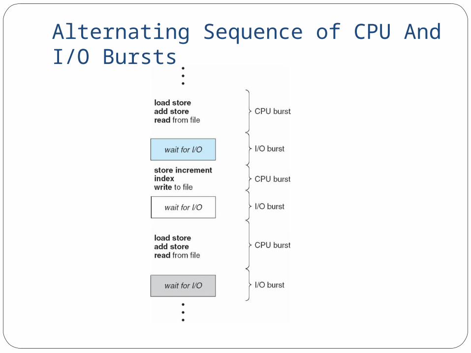
Alternating Sequence of CPU And I/O Bursts

CPU SchedulerSelects from among the processes in

memory that are ready to execute, and allocates the CPU to one of them

CPU scheduling decisions may take place when a process:1. Switches from running to waiting state2. Switches from running to ready state3. Switches from waiting to ready4. Terminates

Scheduling under 1 and 4 is nonpreemptiveAll other scheduling is preemptive

DispatcherDispatcher module gives control of the CPU

to the process selected by the short-term scheduler; this involves:switching contextswitching to user modejumping to the proper location in the user

program to restart that programDispatch latency – time it takes for the

dispatcher to stop one process and start another running

Scheduling CriteriaCPU utilization – keep the CPU as busy as

possibleThroughput – # of processes that complete

their execution per time unitTurnaround time – amount of time to execute

a particular processWaiting time – amount of time a process has

been waiting in the ready queueResponse time – amount of time it takes from

when a request was submitted until the first response is produced, not output (for time-sharing environment)

Scheduling Algorithm Optimization CriteriaMax CPU utilizationMax throughputMin turnaround time Min waiting time Min response time

P1 P2 P3

24 27 300

First-Come, First-Served (FCFS) Scheduling

Process Burst Time P1 24 P2 3 P3 3

Suppose that the processes arrive in the order: P1 , P2 , P3 The Gantt Chart for the schedule is:

Waiting time for P1 = 0; P2 = 24; P3 = 27Average waiting time: (0 + 24 + 27)/3 = 17

FCFS Scheduling (Cont)Suppose that the processes arrive in the order

P2 , P3 , P1 The Gantt chart for the schedule is:

Waiting time for P1 = 6; P2 = 0; P3 = 3Average waiting time: (6 + 0 + 3)/3 = 3Much better than previous caseConvoy effect short process behind long process

P1P3P2

63 300

Shortest-Job-First (SJF) SchedulingAssociate with each process the length of

its next CPU burst. Use these lengths to schedule the process with the shortest time

SJF is optimal – gives minimum average waiting time for a given set of processesThe difficulty is knowing the length of the

next CPU request

Example of SJFProcess Burst Time

P1 6

P2 8

P3 7

P4 3SJF scheduling chart

Average waiting time = (3 + 16 + 9 + 0) / 4 = 7

P4 P3P1

3 160 9

P2

24

Priority SchedulingA priority number (integer) is associated with

each processThe CPU is allocated to the process with the

highest priority (smallest integer highest priority)PreemptiveNon preemptive

SJF is a priority scheduling where priority is the predicted next CPU burst time

Problem Starvation – low priority processes may never execute

Solution Aging – as time progresses increase the priority of the process

Round Robin (RR)Each process gets a small unit of CPU time (time

quantum), usually 10-100 milliseconds. After this time has elapsed, the process is preempted and added to the end of the ready queue.

If there are n processes in the ready queue and the time quantum is q, then each process gets 1/n of the CPU time in chunks of at most q time units at once. No process waits more than (n-1)q time units.

Performanceq large FIFOq small q must be large with respect to context

switch, otherwise overhead is too high

P1 P2 P3 P1 P1 P1 P1 P1

0 4 7 10 14 18 22 26 30

Example of RR with Time Quantum = 4

Process Burst TimeP1 24 P2 3 P3 3

The Gantt chart is:

Typically, higher average turnaround than SJF, but better response

Time Quantum and Context Switch Time

Turnaround Time Varies With The Time Quantum

Multilevel QueueReady queue is partitioned into separate queues:

foreground (interactive)background (batch)

Each queue has its own scheduling algorithmforeground – RRbackground – FCFS

Scheduling must be done between the queuesFixed priority scheduling; (i.e., serve all from

foreground then from background). Possibility of starvation.

Time slice – each queue gets a certain amount of CPU time which it can schedule amongst its processes; i.e., 80% to foreground in RR

20% to background in FCFS

Multilevel Queue Scheduling

Multilevel Feedback QueueA process can move between the various

queues; aging can be implemented this wayMultilevel-feedback-queue scheduler defined by

the following parameters:number of queuesscheduling algorithms for each queuemethod used to determine when to upgrade a

processmethod used to determine when to demote a

processmethod used to determine which queue a process

will enter when that process needs service

Three queues: Q0 – RR with time quantum 8 millisecondsQ1 – RR time quantum 16 millisecondsQ2 – FCFS

SchedulingA new job enters queue Q0 which is served FCFS.

When it gains CPU, job receives 8 milliseconds. If it does not finish in 8 milliseconds, job is moved to queue Q1.

At Q1 job is again served FCFS and receives 16 additional milliseconds. If it still does not complete, it is preempted and moved to queue Q2.

Example of Multilevel Feedback Queue

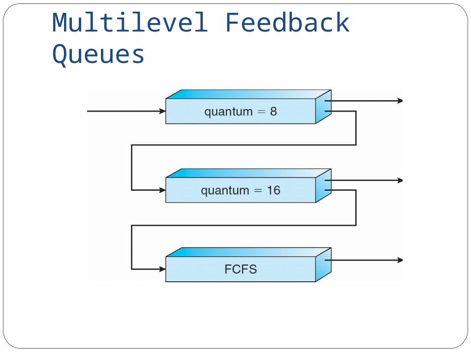
Multilevel Feedback Queues

Thread SchedulingDistinction between user-level and kernel-level

threadsMany-to-one and many-to-many models, thread

library schedules user-level threads to run on LWPKnown as process-contention scope (PCS) since

scheduling competition is within the process

Kernel thread scheduled onto available CPU is system-contention scope (SCS) – competition among all threads in system

Multiple-Processor SchedulingCPU scheduling more complex when multiple CPUs are

availableHomogeneous processors within a multiprocessorAsymmetric multiprocessing – only one processor

accesses the system data structures, alleviating the need for data sharing

Symmetric multiprocessing (SMP) – each processor is self-scheduling, all processes in common ready queue, or each has its own private queue of ready processes

Processor affinity – process has affinity for processor on which it is currently runningsoft affinityhard affinity

Multicore ProcessorsRecent trend to place multiple processor

cores on same physical chipFaster and consume less powerMultiple threads per core also growing

Takes advantage of memory stall to make progress on another thread while memory retrieve happens

Multithreaded Multicore System

End of Lecture 4

Slides adopted from the book:

Abraham Silberschatz, Peter Baer Galvin, Greg Gagne, “Operating System Concepts”, 8/E, John Wiley & Sons, 2010. (ISBN: 978-0-470-23399-3)