18.1 Basic Elements of a Model Query · Web view10/10/2017 · It becomes extremely difficult to solve such problems in SQL, ... Spreadsheet subquery FOR cell index ... Iteration

Chapter 18. Model QueriesSome complex calculations are not easily amenable to SQL. Tasks such as forecasting sales, computing market share, solving simultaneous equations, analyzing time series, and so on involve iterative calculations, often referencing interdependent rows across multiple dimensions. It becomes extremely difficult to solve such problems in SQL, and the resultant SQL code becomes very difficult to understand and maintain. Such SQL often involves multiple levels of subqueries, joins, and UNIONs, and therefore performs inefficiently.Rather than use SQL to solve problems such as we've just described, people usually download the data to a spreadsheet and perform the computations there. Some applications move data into specially created, external calculation engines that can perform the necessary computations efficiently. Downloading data into spreadsheets, or moving data into special-purpose engines, involves overhead and adversely impacts performance, scalability, manageability, and security of the system managing the data.Oracle Database 10g introduces a new MODEL clause that allows you to treat relational data as a multidimensional array for the purpose of performing spreadsheet-like operations. Now you can more easily solve such problems as we've just described, in the database, using a single SQL statement.18.1 Basic Elements of a Model QueryLet's take an example to understand the basic elements of a model query. The sales_history table holds the sales data for three regions for each of the 12 months of the years 2000 and 2001. We want to forecast sales for the first three months of the year 2004, by using a simple formula: the sales for each region for each month of 2004 will be forecasted to be the average sales for that region and that month for years 2000 and 2001. Mathematically, our formula looks as follows:sales_2004 = (sales_2000 + sales_2001) / 2

Using the MODEL clause introduced in Oracle Database 10g, this forecasting model can be written into a SQL query as follows:SELECT r, y, m, s

FROM sales_history

WHERE month <= 3

MODEL

RETURN UPDATED ROWS

PARTITION BY (region_id r)

DIMENSION BY (year y, month m)

MEASURES (sales s)

RULES (s[2004, FOR m in (1,2,3)] = (s[2000,CV( )] + s[2001,CV( )]) / 2)

ORDER BY y, r, m;

R Y M S

---------- ---------- ---------- ----------

2

5 2004 1 763822.5

5 2004 2 923619

5 2004 3 849724.5

6 2004 1 916045.5

6 2004 2 643014

6 2004 3 955546.5

7 2004 1 568531.5

7 2004 2 927634.5

7 2004 3 983989.5

9 rows selected.

The preceding query is called a model query, and introduces some new keywords: MODEL, PARTITION BY, DIMENSION BY, MEASURES, and RULES.The keyword MODEL marks the start of the MODEL clause. The MODEL clause enables you to work with the relational data as a multidimensional array, which is referred to as a model. Once you've arranged your data into an array, you perform spreadsheet-like calculations.The PARTITION BY clause defines logical blocks of the model. You can think of the PARTITION BY clause as separating the data into multiple models, each model being of the same structure, but containing a different subset of the data. This is very similar to the effect of the PARTITION BY clause used with the analytical functions discussed in Chapter 13. If you wish to apply the same calculations to multiple subsets of your data, and you wish each subset to be independent of the other, then partition your data such that each partition corresponds to one of those subsets.The DIMENSION BY clause specifies the dimensions of the multidimensional array created by the MODEL clause. The columns in the DIMENSION BY clause uniquely identify a cell in a partition of the multidimensional array. The dimensions in a model query are equivalent to the dimensions in a star schema. In the example under discussion, the columns year and month are specified as the dimensions, which indicates that each partition will be a two-dimensional array, and a combination of year and the month values will identify each cell.The columns specified in the MEASURES clause are the columns on which the spreadsheet calculations are performed. Measures in a model query are equivalent to the measures in the fact table of a star schema. In our example in this section, the sales column is identified as the measure, and the spreadsheet calculations (estimating future sales) are performed on that column.

Each cell in the model contains the values specified by the MEASURES clause. Our example here uses one value per cell, but later you'll see examples with multiple values per cell.

The RULES keyword introduces the clause specifying the formulae for calculations that you wish to perform. We'll talk more about rules in Section 18.3.

mk:@MSITStore:G:%5C_____Gramatas_un_pasutisana%5CSQL%5CPamati%5C_A_Beaulieu_Mastering_Oracle_SQL_2004.chm::/0596006322/mastorasql2-CHP-18-SECT-3.html#mastorasql2-CHP-18-SECT-3

mk:@MSITStore:G:%5C_____Gramatas_un_pasutisana%5CSQL%5CPamati%5C_A_Beaulieu_Mastering_Oracle_SQL_2004.chm::/0596006322/mastorasql2-CHP-13.html#mastorasql2-CHP-13

3

When you execute a MODEL query, the MODEL clause is almost the last clause to be executed. Only SELECT and ORDER BY come later. Thus, to see the data feeding into a model, you need only remove the MODEL clause, execute the remaining query, and look at the output.A discussion of aliases is in order. Look carefully at the preceding query, and you'll see that aliases are specified in both the SELECT and MODEL clauses. The SELECT and ORDER BY clauses "see" the data that is returned from the MODEL clause. Thus, when you give a column an alias in your MODEL clause, you must use that same alias to refer to the column in your SELECT and ORDER BY clauses. Your SELECT clause may provide yet another alias, which will become the column name "seen" by the user or application program executing the query.18.2 Cell ReferencesReferencing cells in a spreadsheet is one of the basic requirements of model queries. You reference a cell by qualifying all the dimensions in a partition. Cells in a spreadsheet can be referenced in one of the two ways—symbolic cell referencing and positional cell referencing.18.2.1 Symbolic Cell ReferencesIn a symbolic cell reference, you specify each dimension using a boolean expression, such as:s[y=2004, m=3]

An example query with a symbolic cell reference is:SELECT r, y, m, s

FROM sales_history

WHERE month <= 10

MODEL

RETURN UPDATED ROWS



MEASURES (sales s)

RULES (s[y=2004,m=3] = 200000)

ORDER BY y, r, m;

Look at the RULES clause in this example, and see that each cell is referenced symbolically by specifying a value for each dimension. In the RULES clause, s refers to the measure sales declared in the MEASURES clause. This measure is structured in a two-dimensional array, as defined by the DIMENSION BY clause. The dimensions are year (y) and month (m). To reference any cell in the two-dimensional array, you need to specify both the dimensions. In the preceding example, the cell for March 2004 is referenced by specifying a value for the year dimension (y=2004) and the month dimension (m=3). You need to specify the dimensions in the same order as they appear in the DIMENSION BY clause.18.2.2 Positional Cell ReferencesIn a positional cell reference, each dimension is implied by its position in the DIMENSION BY clause. The example from the previous section can be rewritten using positional cell reference as follows:s[2004,3]

An example query with a positional cell reference is:

4

SELECT r, y, m, s

FROM sales_history

WHERE month <= 10

MODEL

RETURN UPDATED ROWS



MEASURES (sales s)

RULES (s[2004,3] = 200000)

ORDER BY y, r, m;

In this query's RULES clause each cell is referenced positionally by specifying a value corresponding to each column listed in the DIMENSION BY clause. Since the DIMENSION BY clause has two columns (year y, month m), the first value in s[2004,3] refers to the column year, and the second value refers to the column month.18.2.3 Combined Positional and Symbolic ReferencesYou may write queries containing both positional and symbolic cell referencing. For example:SELECT r, y, m, s

FROM sales_history

WHERE month <= 10

MODEL

RETURN UPDATED ROWS



MEASURES (sales s)

RULES (s[2004, m=3] = (s[2000,m=3] + s[2001,m=3]) / 2)

ORDER BY y, r, m;

In this query, the RULES clause, s[2004, m=3], contains both positional and symbolic cell referencing. The first dimension (year) is specified positionally, whereas the second dimension (month) is specified symbolically.18.2.4 NULL Measures and Missing CellsSQL models may involve two types of non-available value: existing cells with a NULL value, and non-existing cells. In the MODEL clause, any missing cells are treated as NULLs. Whether they are

5

missing or existing cells with NULL values, the MODEL clause allows you to treat them in either of two ways—IGNORE or KEEP.You can keep the NULL values by specifying KEEP NAV in the MODEL clause. KEEP NAV is the default behavior. Alternatively, you can specify IGNORE NAV in the MODEL clause to return the following values for NULL, depending on the data type of the measure: 0 for numeric data types 01-JAN-2000 for datetime (DATE, TIMESTAMP, etc.) data types An empty string for character (CHAR, VARCHAR2, etc.) data types NULL for all other data typesThe following two examples illustrate the usage of KEEP NAV and IGNORE NAV. The sales history data in the table sales_history has NULL values for the month 12. Therefore, the following query returns NULL values for the measure s:SELECT r, y, m, s

FROM sales_history

WHERE month = 12

MODEL

RETURN UPDATED ROWS



MEASURES (sales s)

RULES (s[2004,12] = (s[2000,12] + s[2001,12]) / 2)

ORDER BY y, r, m;

R Y M S

----- ---------- ---------- ----------

5 2004 12

6 2004 12

7 2004 12

As you can see KEEP NAV is the default behavior. If you want zeros instead of the NULL values for the computed measure s, you can use the IGNORE NAV option in the MODEL clause, as shown in the following example:SELECT r, y, m, s

FROM sales_history

WHERE month = 12

6

MODEL

IGNORE NAV

RETURN UPDATED ROWS



MEASURES (sales s)

RULES (s[2004,12] = (s[2000,12] + s[2001,12]) / 2)

ORDER BY y, r, m;

R Y M S

----- ---------- ---------- ----------

5 2004 12 0

6 2004 12 0

7 2004 12 0

Whether you choose to keep or ignore NULL values depends on your application.18.2.5 UNIQUE DIMENSION/UNIQUE SINGLE REFERENCEThere are two ways to specify the uniqueness of the rows in a MODEL query. The default option is to use UNIQUE DIMENSION, which means that the combination of columns in the PARTITION BY and DIMENSION BY forms the unique key of the input data. When you don't specify any uniqueness condition, or when you specify UNIQUE DIMENSION, the database engine performs a check on the input data to ensure that each cell of the model has at most one row for each combination of PARTITION BY and DIMENSION BY columns. For example:SELECT r, y, m, s

FROM sales_history

WHERE month <= 3

MODEL

UNIQUE DIMENSION



MEASURES (sales s)

7

RULES (s[2004, 3] = (s[2000,3] + s[2001,3]) / 2)

ORDER BY y, r, m;

R Y M S

----- ---------- ---------- ----------

5 2000 1 1018430

5 2000 2 1231492

5 2000 3 1132966

6 2000 1 1221394

6 2000 2 857352

6 2000 3 1274062

7 2000 1 758042

7 2000 2 1236846

7 2000 3 1311986

5 2001 1 509215

5 2001 2 615746

5 2001 3 566483

6 2001 1 610697

6 2001 2 428676

6 2001 3 637031

7 2001 1 379021

7 2001 2 618423

7 2001 3 655993

5 2004 3 849724.5

6 2004 3 955546.5

7 2004 3 983989.5

8

If you are sure that your input data is keyed on the PARTITION BY and DIMENSION BY columns, you can specify UNIQUE SINGLE REFERENCE instead of UNIQUE DIMENSION. When you specify UNIQUE SINGLE REFERENCE, the database engine will not perform the uniqueness check on the entire input data. Rather it will check that all the cells referenced in the righthand side of the rules each correspond to just one row of input data. The reduced checking done by the UNIQUE SINGLE REFERENCE option may improve performance when querying large amounts of data. The following example illustrates the usage of the UNIQUE SINGLE REFERENCE option:SELECT r, y, m, s

FROM sales_history

WHERE month <= 3

MODEL

UNIQUE SINGLE REFERENCE



MEASURES (sales s)

RULES (s[2004, 3] = (s[2000,3] + s[2001,3]) / 2)

ORDER BY y, r, m;

R Y M S

----- ---------- ---------- ----------

5 2000 1 1018430

5 2000 2 1231492

5 2000 3 1132966

6 2000 1 1221394

6 2000 2 857352

6 2000 3 1274062

7 2000 1 758042

7 2000 2 1236846

7 2000 3 1311986

9

5 2001 1 509215

5 2001 2 615746

5 2001 3 566483

6 2001 1 610697

6 2001 2 428676

6 2001 3 637031

7 2001 1 379021

7 2001 2 618423

7 2001 3 655993

5 2004 3 849724.5

6 2004 3 955546.5

7 2004 3 983989.5

If you are using UNIQUE DIMENSION, and the input data doesn't satisfy the uniqueness condition of the PARTITION BY and DIMENSION BY columns, you will get an error, as illustrated in the following example:SELECT r, y, m, s

FROM sales_history

WHERE month >= 10

MODEL

UNIQUE DIMENSION



MEASURES (sales s)

RULES (s[2004, 10] = (s[2000,10] + s[2001,10]) / 2)

ORDER BY y, r, m;

FROM sales_history

*

ERROR at line 2:

10

ORA-32638: Non unique addressing in spreadsheet dimensions

This example returns an error because, in our example data, we have deliberately created duplicate rows for November 2000 and 2001. It doesn't matter that we aren't referencing data from that month in our rule. The duplication causes an error, because data for that month represents a cell somewhere in our model.The same query with the UNIQUE SINGLE REFERENCE option will not cause any error, because the cells referenced in the righthand side of the rules satisfy the required uniqueness condition:SELECT r, y, m, s

FROM sales_history

WHERE month >= 10

MODEL




MEASURES (sales s)

RULES (s[2004, 10] = (s[2000,10] + s[2001,10]) / 2)

ORDER BY y, r, m;

R Y M S

----- ---------- ---------- ----------

5 2000 10 1099296

5 2000 11 922790

5 2000 11 922790

5 2000 12

6 2000 10 1020234

6 2000 11 1065778

6 2000 11 1065778

6 2000 12

7 2000 10 1073682

11

7 2000 11 1107732

7 2000 11 1107732

7 2000 12

5 2001 10 549648

5 2001 11 461395

5 2001 11 461395

5 2001 12

6 2001 10 510117

6 2001 11 532889

6 2001 11 532889

6 2001 12

7 2001 10 536841

7 2001 11 553866

7 2001 11 553866

7 2001 12

5 2004 10 824472

6 2004 10 765175.5

7 2004 10 805261.5

Notice the duplicate rows of data in the above output for month 11 in the years 2000 and 2001. If our rules referenced that data, the query would have caused an error. For example:SELECT r, y, m, s

FROM sales_history

WHERE month >= 10

MODEL




12

MEASURES (sales s)

RULES (s[2004, 11] = (s[2000,11] + s[2001,11]) / 2)

ORDER BY y, r, m;

FROM sales_history

*

ERROR at line 2:

ORA-32638: Non unique addressing in spreadsheet dimensions

This query fails, because there are multiple input rows for a single cell referenced by the rule. Which of the available rows for a given cell should the database choose to use? The answer is that the database doesn't know the answer. That's why the database throws an error. Without this checking for duplicate rows, the database would not be able to guarantee repeatable results.18.2.6 Returning RowsThe objective of all SQL queries is to return a result set. With a model query, you have two options: you can choose to return all the rows represented in the model, or you can choose to return only those rows updated by the rules. Returning all the rows is the default behavior. Use the following clause to specify which behavior you desire:RETURN [ALL | UPDATED] ROWS

The RETURN clause belongs immediately after the MODEL keyword, except when you are using any cell reference options such as IGNORE NAV, KEEP NAV, UNIQUE DIMENSION, or UNIQUE SINGLE REFERENCE. If you are using cell reference options, then those cell reference options need to come before the RETURN clause.The following example illustrates the default behavior:SELECT r, y, m, s

FROM sales_history

WHERE month = 3

MODEL



MEASURES (sales s)

RULES (s[2004,3] = (s[2000,3] + s[2001,3]) / 2)

ORDER BY y, r, m;

R Y M S

13

----- ---------- ---------- ----------

5 2000 3 1132966

6 2000 3 1274062

7 2000 3 1311986

5 2001 3 566483

6 2001 3 637031

7 2001 3 655993

5 2004 3 849724.5

6 2004 3 955546.5

7 2004 3 983989.5

The sales_history table has rows for the year 2000 and 2001. The rows for the year 2004 are computed based on the rules. Since the query didn't specify a RETURN clause, all the rows that satisfy the WHERE condition are returned.To return only updated rows, use the RETURN UPDATED ROWS option, as in the following MODEL query:SELECT r, y, m, s

FROM sales_history

WHERE month = 3

MODEL

RETURN UPDATED ROWS



MEASURES (sales s)

RULES (s[2004,3] = (s[2000,3] + s[2001,3]) / 2)

ORDER BY y, r, m;

R Y M S

----- ---------- ---------- ----------

14

5 2004 3 849724.5

6 2004 3 955546.5

7 2004 3 983989.5

This time, only the new rows generated by the query are returned. For the purpose of the RETURN clause, the newly generated rows are also considered "UPDATED ROWS." If the model query had updated some existing rows, those rows would also have been returned in the result set.18.3 RulesRules are the core of a model query. Rules specify the formulae to compute values for the cells in the spreadsheet. Use the RULES clause to specify the rules for a model query. The RULES clause encloses all the rules in parentheses, and each rule is separated from the next by a comma.18.3.1 Constructing a RuleEach rule represents an assignment, and consists of a lefthand side and a righthand side. The RULES clause of one of the previous examples looks like the following:RULES (s[2004,3] = (s[2000,3] + s[2001,3]) / 2)

The lefthand side of a rule (s[2004,3] in this example) identifies the cells to be updated using values from the righthand side of the rule. The righthand side of a rule is an expression that represents the computation to be performed. You can use any valid SQL operator or function in an expression. There are also some additional constructs that you can use in rules, that are specific to the MODEL clause.18.3.1.1 CV( )You can use the CV( ) function in the righthand side of a rule. It returns the current value of a dimension column from the lefthand side of the rule. The following example illustrates:SELECT r, y, m, s

FROM sales_history

WHERE month = 3

MODEL

RETURN UPDATED ROWS



MEASURES (sales s)

RULES (s[2004,3] = (s[2000,CV( )] + s[2001,CV( )]) / 2)

ORDER BY y, r, m;

R Y M S

----- ---------- ---------- ----------

5 2004 3 849724.5

15

6 2004 3 955546.5

7 2004 3 983989.5

The CV( ) function evaluates to the current value of the corresponding dimension. In this example, CV( ) evaluates to 3, corresponding to the month dimension specified on the lefthand side of the rule. The CV( ) function comes in handy when you need to evaluate a rule multiple times, and each time a dimension column takes a different value (such as in FOR loops, discussed later).Optionally, the CV( ) function can take a dimension column as an argument. For example, we could have written CV(m) to access the current month value from the lefthand side of our rule. When no argument is specified, positional referencing is used, which means that the dimension column in the corresponding position is used.18.3.1.2 ANYANY can be used as a wildcard in a rule written with positional referencing. It accepts any value for the corresponding column (including NULL). The following example illustrates the usage of ANY:SELECT r, y, m, s

FROM sales_history

WHERE month <= 3

MODEL

RETURN UPDATED ROWS



MEASURES (sales s)

RULES (s[ANY,3] = (s[CV( ),1] + s[CV( ),2]) / 2)

ORDER BY y, r, m;

R Y M S

----- ---------- ---------- ----------

5 2000 3 1124961

6 2000 3 1039373

7 2000 3 997444

5 2001 3 562480.5

6 2001 3 519686.5

16

7 2001 3 498722

In this example, ANY is used as a wildcard for the year dimension, which translates into "all the values for the column year in the sales_history table." This example also illustrates why CV( ) is so important. Our rule will update every cell for March (month = 3), regardless of the year. We use CV( ) on the righthand side to capture the current year, so that we can reference the values for January and February of that same year.

The use of ANY wildcard prevents cell insertion. We talk more about cell insertion in Section 18.3.4.

18.3.1.3 FOR loopsFOR loops allow you to write a "rule" that affects a number of cells, and acts like a FOR loop in a procedural language such as PL/SQL. FOR loops are expanded at compile-time, so what looks like one rule to you is really seen by the database as many rules. More on this in a bit.FOR loops are allowed only in the lefthand side of a rule. FOR loops allow multiple cells to be inserted by a single rule. FOR loops can take one of the following three forms:FOR d IN (subquery | list)

FOR d [LIKE pattern] FROM v1 TO v2 [INCREMENT | DECREMENT] n

FOR (d1, d2, . . . ) IN (multi_column_subquery | multi_column_list)

The syntax elements are:

d A single-dimension column.

subquery A subquery returning value(s) for the dimension column.

list A list of value(s) for the dimension column.

pattern A string with a %. This pattern behaves slightly differently from the LIKE pattern used in a WHERE clause predicate. This pattern doesn't accept underscore. Values from v1 through v2 are substituted into the pattern at the position marked by %.

v1, v2 Two literals specifying the upper and lower bound for the dimension d.

n A number to increment or decrement by. The value n must be positive.

d1, d2, ... Multiple-dimension columns in a FOR loop.

multi_column_subquery A subquery returning values for the multiple-dimension columns.

mk:@MSITStore:G:%5C_____Gramatas_un_pasutisana%5CSQL%5CPamati%5C_A_Beaulieu_Mastering_Oracle_SQL_2004.chm::/0596006322/mastorasql2-CHP-18-SECT-3.html#mastorasql2-CHP-18-SECT-3.4

17

multi_column_list A list of values for the multiple-dimension columns.The following example illustrates a single-column FOR loop:SELECT r, y, m, s

FROM sales_history

WHERE month <= 6

MODEL

RETURN UPDATED ROWS



MEASURES (sales s)

RULES

(

s[2004,

FOR m IN (SELECT DISTINCT month FROM sales_history WHERE month <= 6)]

= s[2000,CV( )]

)

ORDER BY y, r, m;

R Y M S

------ ---------- ---------- ----------

5 2004 1 1018430

5 2004 2 1231492

5 2004 3 1132966

5 2004 4 1195244

5 2004 5 1132570

5 2004 6 1006708

6 2004 1 1221394

18

6 2004 2 857352

6 2004 3 1274062

6 2004 4 1082292

6 2004 5 1185870

6 2004 6 1002970

7 2004 1 758042

7 2004 2 1236846

7 2004 3 1311986

7 2004 4 1220034

7 2004 5 1322188

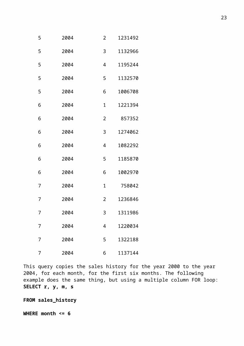
7 2004 6 1137144

This query copies the sales history for the year 2000 to the year 2004, for each month, for the first six months. The following example does the same thing, but using a multiple column FOR loop:SELECT r, y, m, s

FROM sales_history

WHERE month <= 6

MODEL

RETURN UPDATED ROWS



MEASURES (sales s)

RULES

(

s[FOR (y,m)

IN (SELECT DISTINCT 2004, month FROM sales_history WHERE month <= 6)]

= s[2000,CV( )]

)

19

ORDER BY y, r, m;

R Y M S

----- ---------- ---------- ----------

5 2004 1 1018430

5 2004 2 1231492

5 2004 3 1132966

5 2004 4 1195244

5 2004 5 1132570

5 2004 6 1006708

6 2004 1 1221394

6 2004 2 857352

6 2004 3 1274062

6 2004 4 1082292

6 2004 5 1185870

6 2004 6 1002970

7 2004 1 758042

7 2004 2 1236846

7 2004 3 1311986

7 2004 4 1220034

7 2004 5 1322188

7 2004 6 1137144

The following restrictions apply to subqueries used in FOR loops: They cannot be correlated. They cannot be defined using the WITH clause. They cannot return more than 10,000 rows.The last restriction needs more explanation. The total number of rules you can specify in the RULES clause is 10,000. When you use a FOR loop, the RULES clause is expanded by unfolding the FOR loop at compile-time, with the database creating one rule for each value returned by the FOR loop. If

20

the total number of rules, including those not generated from FOR loops, exceeds 10,000 for a given model query, you will get an error. The following example illustrates this error:SELECT r, y, m, s

FROM sales_history

MODEL

RETURN UPDATED ROWS



MEASURES (sales s)

RULES

(

s[2004, FOR m IN (SELECT ROWNUM

FROM orders o1 CROSS JOIN orders o2

WHERE ROWNUM <= 10001)]

= s[2000,CV( )]

)

ORDER BY y, r, m;

SELECT r, y, m, s

*

ERROR at line 1:

ORA-32633: Spreadsheet subquery FOR cell index returns too many rows

In this example, the FOR loop is forced to execute 10,001 times, resulting in 10,001 rules being created, which exceeds the 10,000 rule limit. Even though the error message indicates that the limit is on the subquery of the FOR loop, the limit is actually on the total number of rules in the model. The subquery is simply the component of the model query that caused the limit to be exceeded. If a subquery returns less than 10,000 rows, but the total number of rules after unfolding all the FOR loops still exceeds 10,000, you will get an error, as illustrated in the following example:SELECT r, y, m, s

FROM sales_history

MODEL

21

RETURN UPDATED ROWS



MEASURES (sales s)

RULES

(




= s[2000,CV( )],




= s[2001,CV( )]

)

ORDER BY y, r, m;


*

ERROR at line 14:

ORA-32636: Too many rules in spreadsheet

In this example, one FOR loop results in 5000 rules, and the other FOR loop results in 5001 rules, which make a total of 10001 rules. Therefore, you get the error message that indicates that you have too many rules.18.3.1.4 IS ANYIS ANY can be used as a wildcard in a rule when using symbolic referencing. It accepts any value for the corresponding column (including NULL), and returns TRUE always. This is the equivalent to the ANY wildcard used in positional referencing. IS ANY can be used only in the lefthand side of a rule. The following example illustrates the usage of IS ANY:SELECT r, y, m, s

FROM sales_history

22

WHERE month = 3

MODEL



MEASURES (sales s)

RULES (s[y IS ANY, m=3] = (s[CV( ),m=3] + s[CV( ),m=3]) / 2)

ORDER BY y, r, m;

R Y M S

----- ---------- ---------- ----------

5 2000 3 1132966

6 2000 3 1274062

7 2000 3 1311986

5 2001 3 566483

6 2001 3 637031

7 2001 3 655993

In this example, IS ANY is used as a wildcard for the year dimension, which translates into "all the values for the column year in the sales_history table."

The use of the IS ANY wildcard prevents cell insertion. We talk more about cell insertion in Section 18.3.4.

18.3.1.5 IS PRESENTIS PRESENT returns TRUE if the cell referenced existed prior to the execution of the MODEL clause. Otherwise, if the cell was created as a result of executing a rule, or does not exist at all, IS PRESENT returns FALSE. The following example illustrates the usage of the IS PRESENT condition:SELECT r, y, m, s

FROM sales_history

WHERE month = 3

MODEL


mk:@MSITStore:G:%5C_____Gramatas_un_pasutisana%5CSQL%5CPamati%5C_A_Beaulieu_Mastering_Oracle_SQL_2004.chm::/0596006322/mastorasql2-CHP-18-SECT-3.html#mastorasql2-CHP-18-SECT-3.4

23


MEASURES (sales s)

RULES (s[2004, 3] = CASE WHEN s[2003,3] IS PRESENT

THEN s[2003,3]

ELSE 0

END)

ORDER BY y, r, m;

R Y M S

----- ---------- ---------- ----------

5 2000 3 1132966

6 2000 3 1274062

7 2000 3 1311986

5 2001 3 566483

6 2001 3 637031

7 2001 3 655993

5 2004 3 0

6 2004 3 0

7 2004 3 0

In this example the IS PRESENT condition is used from within a CASE expression to test whether the cell s[2003,3] was present prior to execution of the MODEL clause. If the cell s[2003,3] was present, then the value of the cell s[2003,3] is assigned to the new cell s[2004,3]; if the cell s[2003,3] wasn't present, then the value 0 is assigned to s[2004,3]. As you can see from the result set, the referenced cell didn't satisfy the IS PRESENT condition. You can tell that this is the case, because each of the 2004 rows has been given a 0 value for estimated March (m=3) sales.18.3.1.6 PRESENTVThe PRESENTV function returns a value based on the existence of a cell prior to the execution of the MODEL clause. PRESENTV can be used only on the righthand side of a rule and takes the following form:PRESENTV(cell, exp1, exp2)


24

cell A cell reference

exp1, exp2 Expressions that resolve to a value for the cell referencedPRESENTV returns exp1 if the referenced cell existed prior to the execution of the MODEL clause; otherwise, the function returns exp2. The following example does the same thing as the IS PRESENT example in the previous section, but using the PRESENTV function instead of a CASE and IS PRESENT:SELECT r, y, m, s

FROM sales_history

WHERE month = 3

MODEL



MEASURES (sales s)

RULES (s[2004,3] = PRESENTV(s[2003,3], s[2003,3], 0))

ORDER BY y, r, m;

R Y M S

----- ---------- ---------- ----------

5 2000 3 1132966

6 2000 3 1274062

7 2000 3 1311986

5 2001 3 566483

6 2001 3 637031

7 2001 3 655993

5 2004 3 0

6 2004 3 0

7 2004 3 0

25

In this example, the value for the cell s[2004,3] is determined based on whether the cell s[2003,3] existed before the execution of the MODEL clause. If the cell s[2003,3] existed, its value will be assigned to the cell s[2004,3]. If the cell s[2003,3] didn't exist, a value 0 will be assigned to the cell s[2004,3]. As it appears from the result set, the cell s[2003,3] didn't exist in any of the partitions prior to the execution of the MODEL clause. You can tell that this is the case, because each of the 2004 rows has been given a 0 value for estimated March (m=3) sales.18.3.1.7 PRESENTNNVThe syntax of the PRESENTNNV function is of the same form as that of the PRESENTV function, and like PRESENTV, it can be used only on the righthand side of a rule. PRESENTNNV means "present not null value," and returns exp1 if a cell existed prior to the execution of the MODEL clause, and had a NOT NULL value; otherwise, the function returns exp2. The following example illustrates the usage of PRESENTNNV function:SELECT r, y, m, s

FROM sales_history

MODEL


RETURN UPDATED ROWS



MEASURES (sales s)

RULES (s[2004,3] = PRESENTNNV(s[2000,3], s[2000,3], 0))

ORDER BY y, r, m;

R Y M S

--------- ---------- ---------- ----------

5 2004 3 1132966

6 2004 3 1274062

7 2004 3 1311986

The cell s[2000,3] existed prior to the execution of the MODEL clause, and had a NOT NULL value. You can know this, because all occurrences of s[2004,3] are non-zero in the result set.18.3.2 Range References on the Righthand SideIn most of the examples you have seen so far in this chapter, one cell in the righthand side of a rule has been used to assign a value for one cell in the lefthand side. Or, if more than one cell has been used, each cell has been explicitly referenced. However, there are situations in which you want to use a set of cells on the righthand side to assign one value to a cell on the lefthand side. You can do that by

26

using an aggregate function, such as AVG, COUNT, SUM, MAX, MIN, applied to the multiple cells on the righthand side. This is illustrated in the following example:SELECT r, y, m, s

FROM sales_history

MODEL


RETURN UPDATED ROWS



MEASURES (sales s)

RULES (s[2004, 3] = AVG(s)[y BETWEEN 1995 AND 2003,3])

ORDER BY y, r, m;

R Y M S

----- ---------- ---------- ----------

5 2004 3 849724.5

6 2004 3 955546.5

7 2004 3 983989.5

This example uses the syntax AVG(s)[y BETWEEN 1995 AND 2003,3] to generate the average of all March sales (month 3) between 1995 and 2003 inclusive. In our data, this range encompases: s[1995,3], s[1996,3], s[1997,3], s[1998,3], s[1999,3], s[2000,3], s[2001,3], s[2002,3], and s[2003,3]. When you invoke an aggregate function, be sure to place only the measure name within the parentheses. All the dimensions go outside the parentheses.18.3.3 Order of Evaluation of RulesA MODEL clause usually consists of multiple rules. Quite often, those rules are interdependent. Cells computed by one rule are often used as input to other rules. In such cases, it is very important that rules are evaluated in a proper order. To influence the order of rule evaluation, you can qualify the RULES clause using two options: SEQUENTIAL ORDER and AUTOMATIC ORDER. The syntax to use is:RULES [ [SEQUENTIAL | AUTOMATIC] ORDER ]

The following sections describe the difference between these two approaches to the order in which rules are evaluated.18.3.3.1 SEQUENTIAL ORDERIf you don't specify the ordering option in the RULES clause, SEQUENTIAL ORDER is enforced. The rules are evaluated in the order they appear in the RULES clause (also known as, lexical order). The following example illustrates evaluation of the rules in sequential order:

27

SELECT r, y, m, s

FROM sales_history

WHERE month = 3

MODEL

RETURN UPDATED ROWS



MEASURES (sales s)

RULES SEQUENTIAL ORDER

(

s[2002,3] = (s[2000,3] + s[2001,3])/2,

s[2003,3] = s[2002,3] * 1.1

)

ORDER BY y, r, m;

R Y M S

---------- ---------- ---------- ----------

5 2002 3 849724.5

6 2002 3 955546.5

7 2002 3 983989.5

5 2003 3 934696.95

6 2003 3 1051101.15

7 2003 3 1082388.45

In this query, the first rule computes the cell s[2002,3], and the second rule uses the resulting value to compute the cell s[2003,3]. If you reverse the order of the rules, you won't get the same results:SELECT r, y, m, s

FROM sales_history

28

WHERE month = 3

MODEL


RETURN UPDATED ROWS



MEASURES (sales s)

RULES SEQUENTIAL ORDER

(

s[2003,3] = s[2002,3] * 1.1,

s[2002,3] = (s[2000,3] + s[2001,3])/2

)

ORDER BY y, r, m;

R Y M S

---------- ---------- ---------- ----------

5 2002 3 849724.5

6 2002 3 955546.5

7 2002 3 983989.5

5 2003 3

6 2003 3

7 2003 3

Notice the NULL values returned by the cell s[2003,3] in all the partitions, in this example's output. We asked for sequential ordering of the rules, and the rule to compute s[2003,3] appears before the rule to compute s[2002,3]. The rule to compute s[2003,3] uses s[2002,3]. Since the cell s[2002,3] doesn't exist before the second rule is evaluated, it's value is NULL, and the value for s[2003,3] ends up being NULL as well.18.3.3.2 AUTOMATIC ORDERWith AUTOMATIC ORDER, the evaluation order of the rules is determined using a dependency graph. This is done automatically in a way that ensures that a rule computing a new value for a cell is

29

executed prior to that cell being used to supply a value to another rule. All you need to do to get this behavior is to specify AUTOMATIC ORDER after the RULE keyword. The NULL output of the previous example can be avoided by automatic ordering of the rules, as illustrated in the following example:SELECT r, y, m, s

FROM sales_history

WHERE month = 3

MODEL


RETURN UPDATED ROWS



MEASURES (sales s)

RULES AUTOMATIC ORDER

(

s[2003,3] = s[2002,3] * 1.1,

s[2002,3] = (s[2000,3] + s[2001,3])/2

)

ORDER BY y, r, m;

R Y M S

--------- ---------- ---------- ----------

5 2002 3 849724.5

6 2002 3 955546.5

7 2002 3 983989.5

5 2003 3 934696.95

6 2003 3 1051101.15

7 2003 3 1082388.45

30

In this version of the query, the automatic ordering of the rules ensures that the second rule is evaluated before the first rule.A model with automatic ordering of rules is referred to as an automatic order model, whereas a model with sequential ordering of rules is referred to as a sequential order model. In an automatic order model, a cell can be assigned a value only once, because if a cell is assigned a value more than once, the dependency graph will involve a cycle, and rule evaluation will go into an infinite loop. If you attempt to assign a value to a given cell more than once, you will get an error, as in the following example:SELECT r, y, m, s

FROM sales_history

WHERE month = 3

MODEL

RETURN UPDATED ROWS



MEASURES (sales s)

RULES AUTOMATIC ORDER

(

s[2002,3] = (s[2000,3] + s[2001,3])/2,

s[2002,3] = 20000

)

ORDER BY y, r, m;

s[2002,3] = 20000

*

ERROR at line 11:

ORA-32630: multiple assignment in automatic order SPREADSHEET

However, in a sequential order spreadsheet, you can assign a value to a cell more than once. When you do that, you should remember that the last assignment will be reflected in the final outcome of the query, as illustrated in the following example:SELECT r, y, m, s

FROM sales_history

31

WHERE month = 3

MODEL


RETURN UPDATED ROWS



MEASURES (sales s)

RULES

(

s[2002,3] = (s[2000,3] + s[2001,3])/2,

s[2002,3] = 20000

)

ORDER BY y, r, m;

R Y M S

--------- ---------- ---------- ----------

5 2002 3 20000

6 2002 3 20000

7 2002 3 20000

In this example, the initial assignment of the cell s[2002,3] is overwritten by the value 20000 assigned by the last rule in the list. One more thing to notice about this query is that it doesn't specify an ordering option for the rules. Thus, SEQUENTIAL ORDER is used by default.Why not use AUTOMATIC ORDER all the time? Whenever you are sure about the sequence of rules, you should use SEQUENTIAL ORDER. By doing so, you are saving the database from the overhead of building the dependency graph and determining the rule order every time the query is executed. There are also cases, such as when you must assign a value to a cell, and then later assign another value to the same cell, that preclude automatic ordering.18.3.4 Creating and Updating CellsThe rules in the RULES clause allow you to update existing cells, and to create new cells in a model. If the cell specified by the lefthand side of a rule is present in your model, the value for that cell is updated. If the cell doesn't exist, a new row, corresponding to that cell, is inserted into the result set of your model query. The necessary values for the columns other than the measure columns in any newly

32

inserted row will be derived from its partition and dimension values. This is the default semantics, and is known as UPSERT (update or insert) semantics.The alternative to UPSERT semantics is to use UPDATE semantics. You can specify which to use in the RULES clause:RULES [UPSERT | UPDATE] [SEQUENTIAL ORDER | AUTOMATIC ORDER]

In UPDATE semantics, if the cell specified by the lefthand side of a rule is present in the model, it is updated. If the cell doesn't exist, the assignment is ignored.The following example illustrates UPDATE semantics, in which existing cells are updated, and updates to non-existent cells are ignored:SELECT r, y, m, s

FROM sales_history

MODEL


RETURN UPDATED ROWS



MEASURES (sales s)

RULES UPDATE

(

s[2001,3] = 20000,

s[2002,3] = 20000

)

ORDER BY y, r, m;

R Y M S

----- ---------- ---------- ----------

5 2001 3 20000

6 2001 3 20000

7 2001 3 20000

In this example, the model has the cell s[2001,3], and for each of three partitions, for the regions numbered 5, 6, and 7. The first rule arbitrarily stores the value 20000 into the s[2001,3] cell for each

33

region. The second rule attempts to do the same for the cell s[2002,3], but since that cell doesn't already exist in the spreadsheet, the second rule is ignored. This is how UPDATE semantics work.However, with UPSERT semantics, new cells will be inserted for s[2002,3], as illustrated by the following example:SELECT r, y, m, s

FROM sales_history

MODEL


RETURN UPDATED ROWS



MEASURES (sales s)

RULES UPSERT

(

s[2001,3] = 20000,

s[2002,3] = 20000

)

ORDER BY y, r, m;

R Y M S

----- ---------- ---------- ----------

5 2001 3 20000

6 2001 3 20000

7 2001 3 20000

5 2002 3 20000

6 2002 3 20000

7 2002 3 20000

34

With UPSERT semantics, when you specify a previously non-existent cell and assign a value to that cell, the database inserts a new row into the result set by combining the dimension, measure, and partition information.New cells cannot be inserted in the following situations: As a result of using the ANY wildcard on the lefthand side As a result of using symbolic referencing on the lefthand sideThe ANY wildcard is essentially a predicate that filters selected rows from the population of currently existing rows. When you use a predicate in the WHERE clause of a SELECT statement, that predicate can never generate new rows. Likewise, you can't use a predicate to generate new rows in a model.Symbolic referencing is also a predicate, and this is a subtle, but important point to understand. For example, the cell reference s[y=2003, m=3] is loosely equivalent to a WHERE clause such as WHERE y=2003 AND m=3. Such a WHERE clause can never generate new rows , and neither can such a cell reference.18.4 Iterative ModelsIteration is a powerful tool in mathematical modeling. Some applications involving approximate calculations involve iterative computation. Usually developers resort to procedural languages to implement iteration. The MODEL clause provides a way to write iterate code using SQL.At times, you may need to evaluate the rules of a model repeatedly, until some sort of condition is met. MODEL's ITERATE subclause provides the required functionality to iterate rules. The syntax of the ITERATE subclause, which is a part of the RULES clause, is:RULES [UPSERT | UPDATE] [SEQUENTIAL ORDER | AUTOMATIC ORDER]

ITERATE (n) [UNTIL (condition)]


n A positive number specifying the number of iterations.

condition An early-termination condition.The early-termination condition is optional. If specified, the condition is evaluated at the end of every iteration. If you specify an early-termination condition, iteration ends when that condition is satisfied, regardless of whatever value you specify for n.The following example illustrates iteration of rules:SELECT r, y, m, s

FROM sales_history

MODEL


RETURN UPDATED ROWS



MEASURES (sales s)

RULES ITERATE (4)

35

(

s[2001,3] = s[2001,3] / 2

)

ORDER BY y, r, m;

R Y M S

----- ---------- ---------- ----------

5 2001 3 35405.1875

6 2001 3 39814.4375

7 2001 3 40999.5625

In this query, the cell s[2001,3] is computed by dividing s[2001,3] by 2 four times. You can stop the iteration before all four iterations are executed, by using the UNTIL option, as illustrated in the following example:SELECT r, y, m, s

FROM sales_history

MODEL


RETURN UPDATED ROWS



MEASURES (sales s)

RULES ITERATE (4) UNTIL (s[2001,3] < 100000)

(

s[2001,3] = s[2001,3] / 2

)

ORDER BY y, r, m;

36

R Y M S

----- ---------- ---------- ----------

5 2001 3 70810.375

6 2001 3 79628.875

7 2001 3 81999.125

In this latest example, after every iteration, the condition in the UNTIL clause is evaluated. If the condition is false, the next iteration starts; if the condition is true, the iterative evaluation stops. In this case, once the value of the cell s[2001,3] drops below 100,000, the iteration stops. Compare the two preceding examples, and you will find that the second query didn't perform all four iterations.18.4.1 Knowing how many iterations have occurredSometimes it's useful to know how many iterations have occurred. Oracle provides a useful function (also referred to as a system variable) called ITERATION_NUMBER to keep a count of the number of iterations through a set of rules. The function returns the current iteration number. It starts with 0 for the first iteration, and increments by 1 for every subsequent iteration. So, after a query has completed four iterations, ITERATION_NUMBER will return 3 (iterations 0, 1, 2, and 3). The following example illustrates how you can get the iteration number from a query:SELECT r, y, m, s, i

FROM sales_history

MODEL


RETURN UPDATED ROWS



MEASURES (sales s, 0 i)

RULES ITERATE (4) UNTIL (s[2001,3] < 100000)

(

s[2001,3] = s[2001,3] / 2,

i[2001,3] = ITERATION_NUMBER

)

ORDER BY y, r, m;

R Y M S I

37

----- ---------- ---------- ---------- ----------

5 2001 3 70810.375 2

6 2001 3 79628.875 2

7 2001 3 81999.125 2

Returning the iteration number takes a bit of innovative coding. In the preceding example, a new measure called i has been introduced to capture the iteration number. This measure is updated by the output of the function ITERATION_NUMBER at every iteration. Since i doesn't correspond to any column of the table, we initialized the measure i to the constant 0; we did that in the MEASURES clause. We could have used any constant value to initialize i, and the output would still be the same. This is because the initial value of the measure i is updated to 0 during the first iteration, and then incremented by 1 each iteration thereafter.18.4.1.1 Referencing values from the previous iterationAnother useful feature when using iterations is the PREVIOUS function. The PREVIOUS function takes a single cell reference as input, and returns the value of the cell as it existed after the previous iteration, just before the current iteration began. The following example illustrates how you can use the PREVIOUS function to get the value of a cell as it existed after the previous iteration:SELECT r, y, m, s, i

FROM sales_history

MODEL


RETURN UPDATED ROWS



MEASURES (sales s, 'a' i)

RULES ITERATE (4)

UNTIL ( (PREVIOUS(s[2001,3]) - s[2001,3]) < 100000 )

(

s[2001,3] = s[2001,3] / 2,

i[2001,3] = ITERATION_NUMBER

)

ORDER BY y, r, m;

38

R Y M S I

----- ---------- ---------- ---------- -

5 2001 3 70810.375 2

6 2001 3 79628.875 2

7 2001 3 81999.125 2

In this example, the previous value of the cell is compared to the current value after every iteration, and if that difference is less than 100,000, then the iteration stops. The PREVIOUS function provides a very useful means of constructing a termination condition. For problems requiring approximation solutions, you can use this approach to iterate till a point when the difference between the previous value and the current value is less than a threshold. You can then assume you have arrived at a reasonably approximate solution. For example, you could calculate pi to a resolution of 1/1000.Iteration works only with the sequential ordering of rules. If you attempt to use ITERATE along with AUTOMATIC ORDER, you will get an error, as shown in the following example:SELECT r, y, m, s

FROM sales_history

MODEL


RETURN UPDATED ROWS



MEASURES (sales s)

RULES AUTOMATIC ORDER ITERATE (4)

(

s[2001,3] = 20000,

s[2002,3] = s[2001,3] / 2

)

ORDER BY y, r, m;

RULES AUTOMATIC ORDER ITERATE (4)

*

39

ERROR at line 8:

ORA-32607: invalid ITERATE value in SPREADSHEET clause

18.5 Reference ModelsCommercial spreadsheet applications, such as Microsoft Excel, allow you to link cells from one spreadsheet to those in another spreadsheet. The same thing is possible with model queries in the Oracle database. A given model can reference one or more read-only spreadsheets, called reference models.The REFERENCE clause can be used for referencing spreadsheets/models. The syntax of the REFERENCE clause is:REFERENCE name ON (query)

DIMENSION BY (d)

MEASURES (m)

[ref_options]


name A name for the reference model. You use this together with dot notation to reference values from the model.

query A SELECT statement that defines the reference model.

d Dimension column(s) for the reference model.

m Reference column(s) for the reference model.

ref_options Cell referencing options such as IGNORE NAV, KEEP NAV.For example, the following query uses a REFERENCE clause to create a one-dimensional reference model containing monthly adjustment factors. Those adjustment factors are then referenced by the rule in the main part of the MODEL clause:SELECT r, y, m, s

FROM sales_history

MODEL


RETURN UPDATED ROWS

REFERENCE ref_adj ON

40

(SELECT month, factor FROM monthly_sales_adjustment)

DIMENSION BY (month)

MEASURES (factor)



MEASURES (sales s)

RULES

(

s[2004, FOR m in (1,2,3)] = AVG(s)[y BETWEEN 1995 AND 2003,CV(m)]

* ref_adj.factor[CV(m)]

)

ORDER BY y, r, m;

R Y M S

----- ---------- ---------- ----------

5 2004 1 687440.25

5 2004 2 858965.67

5 2004 3 747757.56

6 2004 1 824440.95

6 2004 2 598003.02

6 2004 3 840880.92

7 2004 1 511678.35

7 2004 2 862700.085

7 2004 3 865910.76

Look at the following component in the preceding query: REFERENCE ref_adj ON


41


MEASURES (factor)

This code component defines the reference model, which has its own dimensions and measures. In this case, the reference model is a one-dimensional array filled in with adjustment factors from the monthly_sales_adjustment table. Those factors are dimensioned by month, making it easy to retrieve the adjustment factor for any given month.The cells of the reference model are referenced from the main model in the following lines:s[2004, FOR m in (1,2,3)] = AVG(s)[y BETWEEN 1995 AND 2003,CV(m)]


The cells of the reference model are qualified using the name of the reference model. In this example, we used ref_adj for our reference model name. Thus, the single measure is ref_adj.factor. Use dot notation to qualify a measure name with the name of the reference model containing the measure. The cell reference ref_adj.factor[CV(m)] that you see here retrieves the adjustment factor for each month.When a query contains more than one model, it makes sense to name each model such that it can be distinguished easily. In the preceding example, you saw how to name a reference model. You can actually name the main model, too, by specifying a name along with the MAIN option, as shown in the following example:SELECT r, y, m, s

FROM sales_history

MODEL


RETURN UPDATED ROWS

REFERENCE ref_adj ON



MEASURES (factor)

MAIN sales_forecast



MEASURES (sales s)

RULES

(

42

s[2004, FOR m in (1,2,3)] = AVG(s)[y BETWEEN 1995 AND 2003,CV(m)]


)

ORDER BY y, r, m;

In this example, the main spreadsheet is named sales_forecast. You can name the main spreadsheet irrespective of whether it references other spreadsheets.The following rules and restrictions apply to reference models: The query defining the reference model cannot correlate to the outer (main) query. A reference model cannot have a PARTITION BY clause. Reference models are read-only. You can't update/upsert a cell in the reference model.A model query can have only one main spreadsheet, but many reference spreadsheets.

Documents

18.1 Basic Elements of a Model Query · Web view10/10/2017 · It becomes extremely difficult to solve such problems in SQL, ... Spreadsheet subquery FOR cell index ... Iteration