Embed Size (px)
Citation preview

18Unified design of lineartransceivers for MIMO channels
Daniel Perez Palomar
MIMO communication systems with CSI at both sides of the link can adapt toeach channel realization to optimize the spectral efficiency and/or the reliability ofthe communication. A low-complexity approach with high potential is the use oflinear MIMO transceivers (composed of a linear precoder at the transmitter and alinear equalizer at the receiver). The design of linear transceivers has been studiedfor many years (the first papers dating back to the 1970s) based on very simplecost functions as a measure of the system quality such as the trace of the MSE ma-trix. If more reasonable measures of quality are considered, the problem becomesmuch more complicated due to its nonconvexity and to the matrix-valued vari-ables. Recent results showed how to solve the problem in an optimal way for thefamily of Schur-concave and Schur-convex cost functions. Although this is a quitegeneral result, there are some interesting functions that fall outside of this cate-gory such as the minimization of the average BER when different constellationsare used. In this chapter, these results are further generalized to include any costfunction as a measure of the quality of the system. When the function is convex, theoriginal complicated nonconvex problem with matrix-valued variables can alwaysbe reformulated a simple convex problem with scalar-valued variables. The sim-plified problem can then be addressed under the powerful framework of convexoptimization theory, in which a great number of interesting design criteria can beeasily accommodated and efficiently solved even though closed-form expressionsmay not exist.
18.1. Introduction
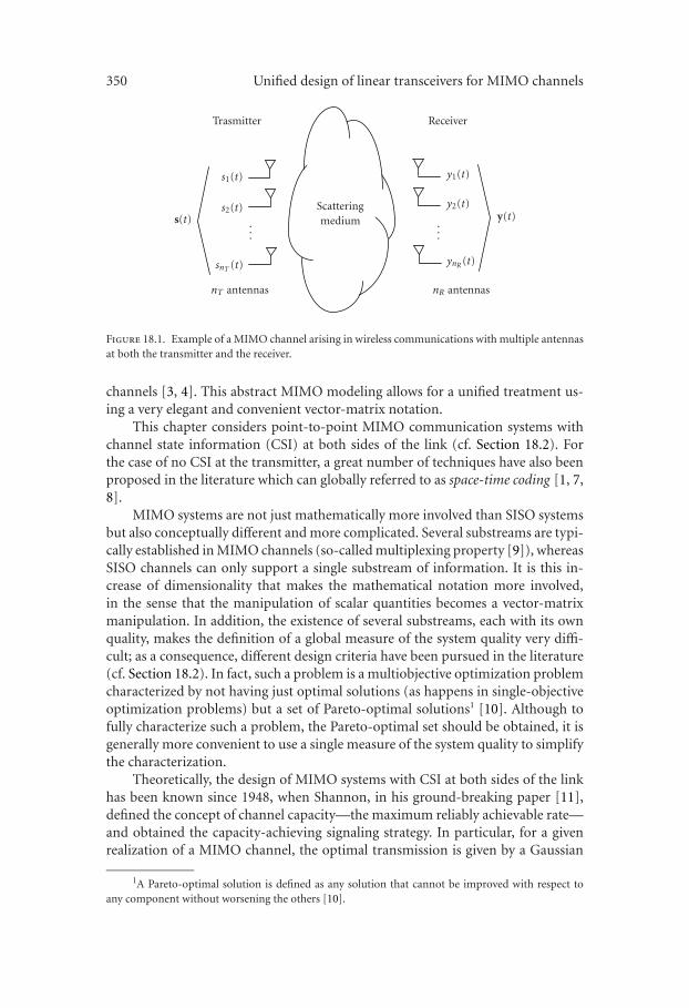
Multiple-input multiple-output (MIMO) channels are an abstract and general wayto model many different communication systems of diverse physical nature; rang-ing from wireless multiantenna channels [1, 2, 3, 4] (see Figure 18.1) to wire-line digital subscriber line (DSL) systems [5], and to single-antenna frequency-selective channels [6]. In particular, wireless multiantenna MIMO channels havebeen recently attracting a significant interest because they provide an importantincrease of spectral efficiency with respect to single-input single-output (SISO)
350 Unified design of linear transceivers for MIMO channels
ReceiverTrasmitter
Scatteringmediums(t) y(t)
s1(t)
s2(t)
...
snT (t)
nT antennas
y1(t)
y2(t)
...
ynR (t)
nR antennas
Figure 18.1. Example of a MIMO channel arising in wireless communications with multiple antennasat both the transmitter and the receiver.
channels [3, 4]. This abstract MIMO modeling allows for a unified treatment us-ing a very elegant and convenient vector-matrix notation.
This chapter considers point-to-point MIMO communication systems withchannel state information (CSI) at both sides of the link (cf. Section 18.2). Forthe case of no CSI at the transmitter, a great number of techniques have also beenproposed in the literature which can globally referred to as space-time coding [1, 7,8].
MIMO systems are not just mathematically more involved than SISO systemsbut also conceptually different and more complicated. Several substreams are typi-cally established in MIMO channels (so-called multiplexing property [9]), whereasSISO channels can only support a single substream of information. It is this in-crease of dimensionality that makes the mathematical notation more involved,in the sense that the manipulation of scalar quantities becomes a vector-matrixmanipulation. In addition, the existence of several substreams, each with its ownquality, makes the definition of a global measure of the system quality very diffi-cult; as a consequence, different design criteria have been pursued in the literature(cf. Section 18.2). In fact, such a problem is a multiobjective optimization problemcharacterized by not having just optimal solutions (as happens in single-objectiveoptimization problems) but a set of Pareto-optimal solutions1 [10]. Although tofully characterize such a problem, the Pareto-optimal set should be obtained, it isgenerally more convenient to use a single measure of the system quality to simplifythe characterization.
Theoretically, the design of MIMO systems with CSI at both sides of the linkhas been known since 1948, when Shannon, in his ground-breaking paper [11],defined the concept of channel capacity—the maximum reliably achievable rate—and obtained the capacity-achieving signaling strategy. In particular, for a givenrealization of a MIMO channel, the optimal transmission is given by a Gaussian
1A Pareto-optimal solution is defined as any solution that cannot be improved with respect toany component without worsening the others [10].

Daniel Perez Palomar 351
signaling with a water-filling power profile over the channel eigenmodes [2, 3, 12].From a more practical standpoint, however, the ideal Gaussian codes are sub-stituted with practical constellations (such as QAM constellations) and codingschemes. To simplify the study of such a system, it is customary to divide it intoan uncoded part, which transmits symbols drawn from some constellations, anda coded part that builds upon the uncoded system. Although the ultimate systemperformance depends on the combination of both parts (in fact, for some systems,such a division does not apply), it is convenient to consider the uncoded and codedparts independently to simplify the analysis and design. The focus of this chapteris on the uncoded part of the system and, specifically, on the employment of lineartransceivers (composed of a linear precoder at the transmitter and a linear equal-izer at the receiver) for complexity reasons.2
Hence, the problem faced when designing a MIMO system not only lies onthe design itself but also on the choice of the appropriate measure of the systemquality (which may depend on the application at hand and/or on the type of cod-ing used on top of the uncoded system). The traditional results existing in theliterature have dealt with the problem from a narrow perspective (due to the com-plexity of the problem); the basic approach has been to choose a measure of qualityof the system sufficiently simple such that the problem can be analytically solved.Recent results have considered more elaborated and meaningful measures of qual-ity. In the sequel, a unified framework for the systematic design of linear MIMOtransceivers is developed.
This chapter is structured as follows. Section 18.2 gives an overview of theclassical and recent results existing in the literature. After describing the signalmodel in Section 18.3, the general problem to be addressed is formulated in Sec-tion 18.4. Then, Section 18.5 gives the optimal receiver and Section 18.6 obtainsthe main result of this chapter: the unified framework for the optimization of thetransmitter under different criteria. Section 18.7 addresses the issue of the diago-nal/nondiagonal structure of the optimal transmission. Several illustrative exam-ples are considered in detail in Section 18.8. The extension of the results to multi-ple MIMO channels is described in Section 18.9. Some numerical results are givenin Section 18.10 to exemplify the application of the developed framework. Finally,Section 18.11 summarizes the main results of the chapter.
The following notation is used. Boldface uppercase letters denote matrices,boldface lowercase letters denote column vectors, and italics denote scalars. Rm×n
and Cm×n represent the set of m × n matrices with real- and complex-valued en-tries, respectively. The superscripts (·)T , (·)∗, and (·)H denote transpose, complexconjugate, and Hermitian operations, respectively. [X]i, j (also [X]i j) denotes the(ith, jth) element of matrix X. Tr(·) and det(·) denote the trace and determinantof a matrix, respectively. A block-diagonal matrix with diagonal blocks given bythe set {Xk} is denoted by diag({Xk}). The operator (x)+ � max(0, x) is the pro-jection onto the nonnegative orthant.
2The choice of linear transceivers is also supported by their optimality from an information-theoretic viewpoint.

352 Unified design of linear transceivers for MIMO channels
18.2. Historical overview of MIMO transceivers
The design of linear MIMO transceivers has been studied since the 1970s wherecable systems were the main application [13, 14]. Initially, since the problem isvery complicated, it was tackled by optimizing easily tractable cost function as ameasure of the system quality such as the sum of the mean square error (MSE)of all channel substreams or, equivalently, the trace of the MSE matrix [6, 13, 14,15]. Others examples include the minimization of the weighted trace of the MSEmatrix [16], the minimization of the determinant of the MSE matrix [17], and themaximization of the signal-to-interference-plus-noise ratio (SINR) criterion witha zero-forcing (ZF) constraint [6]. Some criteria were considered under a peakpower constraint in [18].
For these criteria, the original complicated design problem is greatly simpli-fied because the channel turns out to be diagonalized by the optimal transmit-receive processing and the transmission is effectively performed on a diagonalor parallel fashion. The diagonal transmission allows a scalarization of the prob-lem (meaning that all matrix equations are substituted with scalar ones) withthe consequent simplification. In light of the optimality of the diagonal struc-ture for transmission in all the aforementioned examples (including the capacity-achieving solution [3, 12, 19]), one may expect that the same holds for other cri-teria as well.
In [20], a general unifying framework was developed that embraces a widerange of different design criteria; in particular, the optimal design was obtainedfor the family of Schur-concave and Schur-convex cost functions which arise inmajorization theory [21]. Interestingly, this framework gives a clear answer to thequestion of when the diagonal transmission is optimal.
However, rather than the MSE or the SINR, the ultimate performance of asystem is given by the bit error rate (BER), which is more difficult to handle. In[22], the minimization of the BER (and also of the Chernoff upper bound) aver-aged over the channel substreams was treated in detail when a diagonal structureis imposed. Recently, the minimum BER design without the diagonal structureconstraint has been independently obtained in [20, 23], resulting in an optimalnondiagonal structure. This result, however, only applies when the constellationsused in all channel substreams are equal (in which case the cost function hap-pens to be Schur-convex [20]). The general case of different constellations is muchmore involved (in such a case, the cost function is neither Schur-convex nor Schur-concave) and was solved in [24] via a primal decomposition approach.
There are two natural extensions of the existing results on point-to-pointMIMO transceivers: to the case of imperfect CSI and to the multiuser scenario.With imperfect CSI (due, e.g., to estimation errors), robust transceivers are nec-essary to cope with the uncertainty. The existing results along this line are veryfew and further work is still needed; some results were obtained in [25, 26] with aworst-case robust approach and in [27, 28] with a stochastic robust approach (seealso [29] for a combination of space-time coding with linear precoding). Regard-ing the extension to the multiuser scenario, the existing results are very scarce: in

Daniel Perez Palomar 353
B H AH
LnT × L
nTnR × nT
nR nRL× nR
Lx
s
n
yx
Figure 18.2. Scheme of a general MIMO communication system with a linear transceiver.
[30], a suboptimal joint design of the transmit-receive beamforming and powerallocation in a wireless network was proposed; and, in [31], the optimal MIMOtransceiver design in a multiple-access channel was obtained in terms of minimiz-ing the sum of the MSEs of all the substreams and of all users (a similar approachwas employed in [32] for a broadcast channel). Iterative single-user methods havealso been applied to the multiuser case with excellent performance [33, 34].
In the sequel, the problem of linear MIMO transceiver design is formulatedand solved in a very general way for an arbitrary cost function as a measure ofthe system quality. The design can then be approached from a unified perspectivethat provides great insight into the problem and simplifies it. The key step is in re-formulating the originally nonconvex problem in convex form after some manip-ulations based on majorization theory [21]. The simplified problem can then beaddressed under the powerful framework of convex optimization theory [35, 36],in which a great number of interesting design criteria can be easily accommodatedand efficiently solved even though closed-form expressions may not exist.
18.3. System model
The signal model corresponding to a transmission through a general MIMO com-munication channel with nT transmit and nR receive dimensions is
y = Hs + n, (18.1)
where s ∈ CnT×1 is the transmitted vector, H ∈ CnR×nT is the channel matrix, y ∈CnR×1 is the received vector, and n ∈ CnR×1 is a zero-mean circularly symmetriccomplex Gaussian interference-plus-noise vector with arbitrary covariance matrixRn.
The transmitted vector can be written as (see Figure 18.2)
s = Bx, (18.2)
where B ∈ CnT×L is the transmit matrix (precoder) and x ∈ CL×1 is the datavector that contains the L symbols to be transmitted (zero mean,3 normalized anduncorrelated, that is, E[xxH] = I) drawn from a set of constellations. For the sake
3If a constellation does not have zero mean, the receiver can always remove the mean and thenproceed as if the mean was zero, resulting in a loss of transmitted power. Indeed, the mean of the signaldoes not carry any information and can always be set to zero saving power at the transmitter.

354 Unified design of linear transceivers for MIMO channels
of notation, it is assumed that L ≤ min(nR,nT). The total average transmittedpower (in units of energy per transmission) is
PT = E[‖s‖2] = Tr
(BBH). (18.3)
Similarly, the estimated data vector at the receiver is (see Figure 18.2)
x = AHy, (18.4)
where AH ∈ CL×nR is the receive matrix (equalizer).It is interesting to observe that the ith column of B and A, bi and ai, respec-
tively, can be interpreted as the transmit and receive beam vectors, respectively,associated to the ith transmitted symbol xi:
xi = aHi(
Hbixi + ni), (18.5)
where ni =∑
j �=i Hb jx j + n is the equivalent noise seen by the ith substream, withcovariance matrix Rni =
∑j �=i Hb jbH
j HH + Rn.It is worth noting that in some particular scenarios such as in multicarrier
systems, although the previous signal model can be directly applied by properlydefining the channel matrix H as a block-diagonal matrix containing the channelat each carrier, it may also be useful to model the system as a set of parallel andnoninterfering MIMO channels (cf. Section 18.9).
18.3.1. Measures of quality
The quality of the ith established substream or link in (18.5) can be convenientlymeasured, among others, in terms of MSE, SINR, or BER, defined, respectively, as
MSEi � E[∣∣xi − xi
∣∣2] = ∣∣aHi Hbi − 1∣∣2
+ aHi Rniai, (18.6)
SINRi �desired component
undesired component=
∣∣aHi Hbi
∣∣2
aHi Rniai, (18.7)
BERi �# bits in error
# transmitted bits≈ gi
(SINRi
), (18.8)
where gi is a function that relates the BER to the SINR at the ith substream. Formost types of modulations, the BER can indeed be analytically expressed as a func-tion of the SINR when the interference-plus-noise term follows a Gaussian distri-bution [37, 38, 39]; otherwise, it is an approximation (see [24] for a more de-tailed discussion). For example, for square M-ary QAM constellations, the BER is[37, 39]
BER(SINR) ≈ 4log2 M
(1 − 1√
M
)Q
(√3
M − 1SINR
), (18.9)

Daniel Perez Palomar 355
y AH
Detector
...
Detector
nR
L× nR
x1
xL
Figure 18.3. Independent detection of the substreams after the joint linear processing with matrix A.
where Q is the Q-function defined as Q(x) � (1/√
2π)∫∞x e−λ2/2dλ [38].4 It is
sometimes convenient to use the Chernoff upper bound of the tail of the Gauss-ian distribution function Q(x) ≤ (1/2)e−x2/2 [38] to approximate the symbol er-ror probability (which becomes a reasonable approximation for high values of theSINR).
It is worth pointing out that expressing the BER as in (18.8) implicitly assumesthat the different links are independently detected after the joint linear processingwith the receive matrix A (see Figure 18.3). This reduces the complexity drasticallycompared to a joint maximum-likelihood (ML) detection and is indeed the mainadvantage of using the receive matrix A.
Any properly designed system should attempt to somehow minimize theMSEs, maximize the SINRs, or minimize the BERs, as is mathematically formu-lated in the next section.
18.4. General problem formulation
The problem addressed in this chapter is the optimal design of a linear MIMOtransceiver (matrices A and B) as a tradeoff between the power transmitted andthe quality achieved. To be more specific, the problem can be formulated as theminimization of some cost function f0 of the MSEs in (18.6), which measures thesystem quality (a smaller value of f0 means a better quality), subject to a transmitpower constraint [20, 40]:
minA,B
f0({
MSEi})
s.t. Tr(
BBH) ≤ P0
(18.10)
or, conversely, as the minimization of the transmit power subject to a constrainton the quality of the system:
minA,B
Tr(
BBH)s.t. f0
({MSEi
}) ≤ α0,(18.11)
where P0 and α0 denote the maximum values for the power and for the cost func-tion, respectively.
4The complementary error function is related to the Q-function as erfc(x) = 2 Q(√
2x) [38].
356 Unified design of linear transceivers for MIMO channels
The cost function f0 is an indicator of how well the system performs andshould be properly selected for the problem at hand. In principle, any functioncan be used to measure the system quality as long as it is strictly increasing in eachargument. Note that the increasingness of f0 is a mild and completely reasonableassumption: if the quality of one of the substream improves while the rest remainunchanged, any reasonable function should properly reflect this difference.
The problem formulations in (18.10) and (18.11) are in terms of a cost func-tion of the MSEs; however, similar design problems can be straightforwardly for-mulated with cost functions of the SINRs and of the BERs (when using cost func-tions of the BERs, it is implicitly assumed that the constellations have already beenchosen such that (18.8) can be employed).
Alternatively, it is also possible to consider independent constraints on eachof the links rather than a global measure of the quality [26, 40]:
minA,B
Tr(
BBH)s.t. MSEi ≤ ρi 1 ≤ i ≤ L,
(18.12)
where ρi denotes the maximum MSE value for the ith substream. Constraints interms of SINR and BER can be similarly considered. Note that the solution toproblem (18.12) allows a more detailed characterization of the fundamental mul-tiobjective nature of the problem [10]; it allows, for example, to compute the exactregion of achievable MSEs for a given power budget.
For the sake of space, this chapter focuses on the power-constrained prob-lem in (18.10). The quality-constrained problem in (18.11), however, is so closelyrelated that the results obtained also hold for this problem (in particular, Theo-rem 18.1 holds for problem (18.11)). Problem (18.12) is mathematically more in-volved and the interested reader is referred to [24, 26, 40].
If fact, since problems (18.10) and (18.11) characterize the same strictlymonotonic tradeoff curve of power versus quality, each of them can be easily solvedby iteratively solving the other one using, for example, the bisection method [35,Algorithm 4.1].
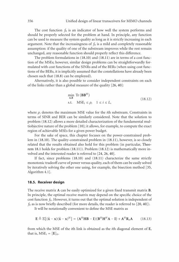
18.5. Receiver design
The receive matrix A can be easily optimized for a given fixed transmit matrix B.In principle, the optimal receive matrix may depend on the specific choice of thecost function f0. However, it turns out that the optimal solution is independent off0 as is now briefly described (for more details, the reader is referred to [20, 40]).
It will be notationally convenient to define the MSE matrix as
E � E[(x − x)(x − x)H
] = (AHHB − I
)(BHHHA − I
)+ AHRnA (18.13)
from which the MSE of the ith link is obtained as the ith diagonal element of E,that is, MSEi = [E]ii.

Daniel Perez Palomar 357
MMSE receiverZF receiver
MSE
BE
R
0 0.02 0.04 0.06 0.08 0.1 0.12 0.14 0.16 0.18 0.20
0.005
0.01
0.015
0.02512-QAM256-QAM128-QAM64-QAM32-QAM
16-QAM8-QAM
QPSK
Figure 18.4. BER as a function of the MSE for different QAM constellations.
The minimization of the MSE of a substream with respect to the receive ma-trix A (for a fixed transmit matrix B) does not incur any penalty on the othersubstreams (see, e.g., (18.5) where ai only affects xi); in other words, there is notradeoff among the MSEs and the problem decouples. Therefore, it is possible tominimize simultaneously all MSEs and this is precisely how the well-known lin-ear minimum MSE (MMSE) receiver, also termed Wiener filter, is obtained [41](see also [20, 26]). If the additional ZF constraint AHHB = I is imposed to avoidcrosstalk among the substreams (which may happen with the MMSE receiver),then the well-known ZF receiver is obtained [40]. Interestingly, the MMSE andZF receivers are also optimum in the sense that they maximize simultaneously allSINRs and, consequently, minimize simultaneously all BERs (cf. [20, 40]).
The MMSE and ZF receivers can be compactly written as
A = R−1n HB
(νI + BHHHR−1
n HB)−1
, (18.14)
where ν is a parameter defined as
ν �1 for the MMSE receiver,
0 for the ZF receiver.(18.15)
The MSE matrix reduces then to the following concentrated MSE matrix:
E = (νI + BHRHB
)−1, (18.16)
where RH � HHR−1n H is the squared whitened channel matrix.
18.5.1. Relation among different measures of quality
It is convenient now to relate the different measures of quality, namely, MSE, SINR,and BER, to the concentrated MSE matrix in (18.16).

358 Unified design of linear transceivers for MIMO channels
From the definition of MSE matrix, the individual MSEs are given by the di-agonal elements:
MSEi =[(νI + BHRHB
)−1]ii. (18.17)
It turns out that the SINRs and the MSEs are trivially related when using theMMSE or ZF receivers as [20, 26, 40]
SINRi = 1MSEi
− ν. (18.18)
Finally, the BERs can also be written as a function of the MSEs:
BERi = gi(
MSEi)
� gi(
SINRi = MSE−1i −ν), (18.19)
where gi was defined in (18.8).It is important to remark that the BER functions gi are convex decreasing in
the SINR and the BER functions gi are convex increasing in the MSE for sufficientlysmall values of the argument (see Figure 18.4) [20, 40] (this last property will bekey when proving later in Section 18.8.2 that the average BER function is Schur-convex). As a rule of thumb, the BER as a function of the MSE is convex for aBER less than 2 × 10⁻² (this is a mild assumption, since practical systems have ingeneral a smaller uncoded BER5); interestingly, for BPSK and QPSK constellations,the BER function is always convex [20, 40].
Summarizing, the MMSE and ZF receivers have been obtained as the opti-mum solution in the sense of minimizing the MSEs, maximizing the SINRs, andminimizing the BERs. In addition, since the SINR and the BER can be expressedas a function of the MSE, (18.18) and (18.19), it suffices to focus on cost functionsof the MSEs without loss of generality.
18.6. Transmitter design
Now that the MMSE and ZF receivers have been obtained as optimal solutions, themain problem addressed in this chapter can be finally formulated: the optimiza-tion of the transmit matrix B for an arbitrary cost function of the MSEs (recall thatcost functions of the SINRs and BERs can always be reformulated as functions ofthe MSEs).
Theorem 18.1. The following complicated nonconvex constrained optimizationproblem:
minB
f0({[(
νI + BHRHB)−1]
ii
})s.t. Tr
(BBH) ≤ P0,
(18.20)
5Given an uncoded bit error probability of at most 10−2 and using a proper coding scheme, codedbit error probabilities with acceptable low values such as 10−6 can be obtained.
Daniel Perez Palomar 359
where f0 : RL → R is an arbitrary cost function (increasing in each argument andminimized when the arguments are sorted in decreasing order6), is equivalent to thesimple problem
minp,ρ
f0(ρ1, . . . , ρL
)s.t.
L∑j=i
1ν + pjλH , j
≤L∑j=i
ρ j , 1 ≤ i ≤ L,
ρi ≥ ρi+1,
L∑j=1
pj ≤ P0,
pi ≥ 0,
(18.21)
where the λH ,i’s are L largest eigenvalues of RH sorted in increasing order λH ,i ≤ λH ,i+1
and ρL+1 � 0. Furthermore, if f0 is a convex function, problem (18.21) is convex andthe ordering constraint ρi ≥ ρi+1 can be removed.
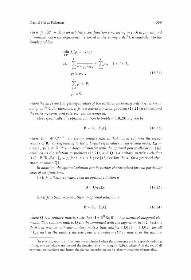
More specifically, the optimal solution to problem (18.20) is given by
B = UH ,1ΣBQ, (18.22)
where UH ,1 ∈ CnT×L is a (semi-)unitary matrix that has as columns the eigen-vectors of RH corresponding to the L largest eigenvalues in increasing order, ΣB =diag({√pi}) ∈ RL×L is a diagonal matrix with the optimal power allocation {pi}obtained as the solution to problem (18.21), and Q is a unitary matrix such that[(νI + BHRHB)−1]ii = ρi for 1 ≤ i ≤ L (see [42, Section IV-A] for a practical algo-rithm to obtain Q).
In addition, the optimal solution can be further characterized for two particularcases of cost functions.
(i) If f0 is Schur-concave, then an optimal solution is
B = UH ,1ΣB. (18.23)
(ii) If f0 is Schur-convex, then an optimal solution is
B = UH ,1ΣBQ, (18.24)
where Q is a unitary matrix such that (I + BHRHB)−1 has identical diagonal ele-ments. This rotation matrix Q can be computed with the algorithm in [42, SectionIV-A], as well as with any unitary matrix that satisfies |[Q]ik| = |[Q]il|, for alli, k, l such as the unitary discrete Fourier transform (DFT) matrix or the unitary
6In practice, most cost functions are minimized when the arguments are in a specific ordering(if not, one can always use instead the function f0(x) = minP∈P f0(Px), where P is the set of allpermutation matrices) and, hence, the decreasing ordering can be taken without loss of generality.

360 Unified design of linear transceivers for MIMO channels
All functionsf : � ⊆ Rn → R
Schur-convexfunctions
Schur-concavefunctions
Figure 18.5. Illustration of the sets of Schur-convex and Schur-concave functions within the set of allfunctions f : A ⊆ Rn → R.
Hadamard matrix (when the dimensions are appropriate such as a power of two [38,page 66]).
Proof . The key simplification from (18.20) to (18.21) is based on an appro-priate change of variable based on majorization theory [21]. A sketch of the proofis given in the appendix (see [20, 40] for details). �
Note that Theorem 18.1 is a generalization of previous results [20, 40] whichonly considered Schur-concave and Schur-convex functions.
Some comments on Theorem 18.1 are in order.(i) The main result is in the simplification of the original complicated problem
(18.20) with a matrix-valued variable to the simple problem (18.21) with a set ofscalar variables that represent a power allocation over the channel eigenvalues. Inother words, the problem has been scalarized in the sense that no matrix appears.
(ii) As stated in the theorem, when f0 is a convex function, then the simplifiedproblem (18.21) is convex. This has tremendous consequences, since the problemcan always be optimally solved using the existing tools in convex optimization the-ory, either in closed-form (using the Karush-Kuhn-Tucker optimality conditions)or at least numerically (using very efficient algorithms recently developed such asinterior-point methods) [35, 36]. Furthermore, additional constraints on the de-sign can be easily incorporated without affecting the solvability of the problem aslong as they are convex (cf. [20, 40]).
(iii) For Schur-concave/convex cost functions, the problem (18.21) is extreme-ly simplified (cf. Sections 18.6.1 and 18.6.2) and in most cases closed-form solu-tions can be obtained (see Section 18.8 for a list of Schur-concave/convex costfunctions and for a detailed treatment of two interesting cases such as the mini-mization of the average BER and the optimization of the worst substream).
(iv) The sets of Schur-concave and Schur-convex functions do no form apartition of the set of all functions as illustrated in Figure 18.5. This means thatthere may be cost functions that are neither Schur-concave nor Schur-convex (cf.Section 18.8.2). On the other hand, there are cost functions that are both Schur-concave and Schur-convex, such as Tr(E), and admit any rotation matrix Q [40].

Daniel Perez Palomar 361
(v) Surprisingly, for Schur-convex cost functions f0, the optimal solution tothe original problem (18.20) is independent of the specific choice of f0 (cf. Sec-tion 18.6.2), as opposed to Schur-concave cost functions, whose solution dependson the particular choice of f0.
(vi) As is explained in detail in Section 18.7, for Schur-concave functions, theoptimal transmission is fully diagonal, whereas for Schur-convex functions, it isnot due to the additional rotation matrix Q (see Figure 18.6)
(vii) For the simple case in which a single substream is established, that is,L = 1, the result in Theorem 18.1 simply means that the eigenmode with highestgain should be used.
18.6.1. Schur-concave cost functions
For Schur-concave cost functions, since the optimal rotation is Q = I (from Theo-rem 18.1), the MSEs are given by
MSEi = 1ν + piλH ,i
, 1 ≤ i ≤ L (18.25)
and the original optimization problem (18.20) can be finally written as
minp
f0
({1
ν + piλH ,i
}i
)
s.t.L∑j=1
pj ≤ P0,
pi ≥ 0, 1 ≤ i ≤ L.
(18.26)
The solution to problem (18.26) clearly depends on the particular choice of f0.
18.6.2. Schur-convex cost functions
For Schur-convex cost functions, since the diagonal elements of E are equal at theoptimal solution (from Theorem 18.1), the MSEs are given by
MSEi = 1L
Tr(E) = 1L
L∑j=1
1ν + pjλH , j
, 1 ≤ i ≤ L (18.27)
and the original optimization problem (18.20) can be finally written as
minp
1L
L∑j=1
1ν + pjλH , j
s.t.L∑j=1
pj ≤ P0,
pi ≥ 0, 1 ≤ i ≤ L.
(18.28)
362 Unified design of linear transceivers for MIMO channels
x1
xL
......
... ...
x1
xL
√p1
√pL
λ1/21
λ1/2L
α1
αL
w1
wL
(a)
x1
xL
... Q...
... ...QH
x1
xL
√p1
√pL
λ1/21
λ1/2L
α1
αL
w1
wL
(b)
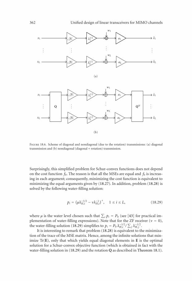
Figure 18.6. Scheme of diagonal and nondiagonal (due to the rotation) transmissions: (a) diagonaltransmission and (b) nondiagonal (diagonal + rotation) transmission.
Surprisingly, this simplified problem for Schur-convex functions does not dependon the cost function f0. The reason is that all the MSEs are equal and f0 is increas-ing in each argument; consequently, minimizing the cost function is equivalent tominimizing the equal arguments given by (18.27). In addition, problem (18.28) issolved by the following water-filling solution:
pi =(µλ−1/2
H ,i − νλ−1H ,i
)+, 1 ≤ i ≤ L, (18.29)
where µ is the water level chosen such that∑
i pi = P0 (see [43] for practical im-plementation of water-filling expressions). Note that for the ZF receiver (ν = 0),the water-filling solution (18.29) simplifies to pi = P0 λ
−1/2H ,i /
∑j λ
−1/2H , j .
It is interesting to remark that problem (18.28) is equivalent to the minimiza-tion of the trace of the MSE matrix. Hence, among the infinite solutions that min-imize Tr(E), only that which yields equal diagonal elements in E is the optimalsolution for a Schur-convex objective function (which is obtained in fact with thewater-filling solution in (18.29) and the rotation Q as described in Theorem 18.1).
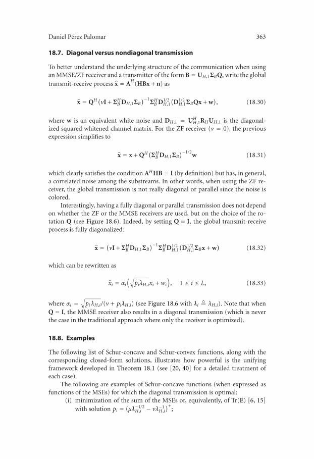
Daniel Perez Palomar 363
18.7. Diagonal versus nondiagonal transmission
To better understand the underlying structure of the communication when usingan MMSE/ZF receiver and a transmitter of the form B = UH ,1ΣBQ, write the globaltransmit-receive process x = AH(HBx + n) as
x = QH(νI + ΣH
B DH ,1ΣB)−1
ΣHB D1/2
H ,1
(D1/2
H ,1ΣBQx + w), (18.30)
where w is an equivalent white noise and DH ,1 = UHH ,1RHUH ,1 is the diagonal-
ized squared whitened channel matrix. For the ZF receiver (ν = 0), the previousexpression simplifies to
x = x + QH(ΣHB DH ,1ΣB
)−1/2w (18.31)
which clearly satisfies the condition AHHB = I (by definition) but has, in general,a correlated noise among the substreams. In other words, when using the ZF re-ceiver, the global transmission is not really diagonal or parallel since the noise iscolored.
Interestingly, having a fully diagonal or parallel transmission does not dependon whether the ZF or the MMSE receivers are used, but on the choice of the ro-tation Q (see Figure 18.6). Indeed, by setting Q = I, the global transmit-receiveprocess is fully diagonalized:
x = (νI + ΣH
B DH ,1ΣB)−1
ΣHB D1/2
H ,1
(D1/2
H ,1ΣBx + w)
(18.32)
which can be rewritten as
xi = αi(√
piλH ,ixi + wi
), 1 ≤ i ≤ L, (18.33)
where αi =√pi λH ,i/(ν + piλH ,i) (see Figure 18.6 with λi � λH ,i). Note that when
Q = I, the MMSE receiver also results in a diagonal transmission (which is neverthe case in the traditional approach where only the receiver is optimized).
18.8. Examples
The following list of Schur-concave and Schur-convex functions, along with thecorresponding closed-form solutions, illustrates how powerful is the unifyingframework developed in Theorem 18.1 (see [20, 40] for a detailed treatment ofeach case).
The following are examples of Schur-concave functions (when expressed asfunctions of the MSEs) for which the diagonal transmission is optimal:
(i) minimization of the sum of the MSEs or, equivalently, of Tr(E) [6, 15]with solution pi = (µλ−1/2
H ,i − νλ−1H ,i
)+;

364 Unified design of linear transceivers for MIMO channels
(ii) minimization of the weighted sum of the MSEs or, equivalently, ofTr(WE) [16], where W = diag({wi}) is a diagonal weighting matrix,with solution pi = (µw1/2
i λ−1/2H ,i − νλ−1
H ,i)+;
(iii) minimization of the (exponentially weighted) product of the MSEs withsolution pi = (µwi − νλ−1
H ,i)+;
(iv) minimization of det(E) [17] with solution pi = (µ− νλ−1H ,i)
+;(v) maximization of the mutual information, for example, [12], with solu-
tion pi = (µ− λ−1H ,i)
+;(vi) maximization of the (weighted) sum of the SINRs with solution given by
allocating all the power on the channel eigenmode with highest weightedgain wi λH ,i;
(vii) maximization of the (exponentially weighted) product of the SINRs withsolution pi = P0 wi/
∑j wj (for the unweighted case, it results in a uni-
form power allocation).The following are examples of Schur-convex functions for which the optimal
transmission is nondiagonal with solution given by pi = (µλ−1/2H ,i − νλ−1
H ,i)+ plus the
rotation Q:(i) minimization of the maximum of the MSEs;
(ii) maximization of the minimum of the SINRs;(iii) maximization of the harmonic mean of the SINRs;7
(iv) minimization of the average BER (with equal constellations);(v) minimization of the maximum of the BERs.
In the following, two relevant examples (with an excellent performance inpractice) are considered to illustrate how easily linear MIMO transceivers can bedesigned with the aid of Theorem 18.1.
18.8.1. Optimization of the worst substream
The optimization of the worst substream can be formulated, for example, as theminimization of the maximum MSE:
minA,B
maxi
{MSEi
}(18.34)
which coincides with the minimization of the maximum BER if equal constella-tions are used. The optimal receive matrix is given by (18.14) and the problemreduces then to
minB
maxi
{[(νI + BHRHB
)−1]ii
}s.t. Tr
(BBH) ≤ P0.
(18.35)
7For the ZF receiver, the maximization of the harmonic mean of the SINRs is equivalent to theminimization of the unweighted sum of the MSEs, which can be classified as both Schur-concave andSchur-convex (since it is invariant to rotations).

Daniel Perez Palomar 365
Theorem 18.1 can now be invoked noting that f0(x) = maxi{xi} is a Schur-convexfunction [20, 40] (if y majorizes x, it must be that xmax ≤ ymax from the definitionof majorization [21, 1.A.1] and, therefore, f0(x) ≤ f0(y) which is precisely thedefinition of Schur-convexity [21, 3.A.1]). Hence, the final problem to be solved is(18.28) with solution given by (18.29) (recall that the rotation matrix Q is neededin this case as indicated in Theorem 18.1).
In light of Theorem 18.1 and the Schur-convexity of the cost function, it isnow clear that the optimal transmission is nondiagonal (cf. Sections 18.6.2 and18.7). However, one can still impose such a structure and solve the original prob-lem in a suboptimal way. The transmit matrix would then be B = UH ,1ΣB and theproblem to be solved in convex form:
minp
t
s.t. t ≥ 1ν + piλH ,i
1 ≤ i ≤ L
L∑j=1
pj ≤ P0
pi ≥ 0
(18.36)
with solution given by pi = P0 λ−1H ,i/
∑j λ
−1H , j .
18.8.2. Minimization of the average BER
The average (uncoded) BER is a good measure of the uncoded part of a system.Hence, its minimization may be regarded as an excellent (if not the best) criterion:
minA,B
1L
L∑i=1
gi(
MSEi), (18.37)
where the functions gi were defined in (18.19) and characterized as convex func-tions (see Figure 18.4). The optimal receive matrix is given by (18.14) and theproblem reduces then to
minB
1L
L∑i=1
gi([(
νI + BHRHB)−1]
ii
)s.t. Tr
(BBH) ≤ P0.
(18.38)
Theorem 18.1 can now be invoked and the problem simplifies to the following

366 Unified design of linear transceivers for MIMO channels
convex problem (provided that the constellations are chosen with increasing car-dinality):
minp,ρ
1L
L∑i=1
gi(ρi)
s.t.L∑j=i
1ν + pjλH , j
≤L∑j=i
ρ j , 1 ≤ i ≤ L,
L∑j=1
pj ≤ P0,
pi ≥ 0.
(18.39)
This particular problem was extensively treated in [24] via a primal decompositionapproach which allowed the resolution of the problem with extremely simple al-gorithms (rather than using general purpose iterative algorithms such as interior-point methods).
In the particular case in which the constellations used in the L substreamsare equal, the average BER cost function turns out to be Schur-convex since itis the sum of identical convex functions [21, 3.H.2]. Hence, the final problem tobe solved is again (18.28) with solution given by (18.29) (recall that the rotationmatrix Q is needed in this case as indicated in Theorem 18.1). As before, the min-imization of the average BER can be suboptimally solved by imposing a diagonalstructure.
18.9. Extension to parallel MIMO channels
As mentioned in Section 18.3, some particular scenarios, such as multicarrier sys-tems, may be more conveniently modeled as a communication through a set ofparallel MIMO channels
yk = Hksk + nk, 1 ≤ k ≤ N , (18.40)
where N is the number of parallel channels and k is the channel index.It is important to remark that a multicarrier system can be modeled, not
only as a set of parallel MIMO channels as in (18.40), but also as a single MIMOchannel as in (18.1) with H = diag({Hk}). The difference lies on whether thetransceiver operates independently at each MIMO channel as implied by (18.40)(block-diagonal matrices B = diag({Bk}) and A = diag({Ak})) or a global tran-sceiver processes jointly all MIMO channels as a whole as implied by (18.1) (fullmatrices B and A).
In the case of a set of N parallel MIMO channels with a single power con-straint per channel, all the results obtained so far for a single MIMO channelclearly hold, since the optimization of a global cost function decouples into a set ofN parallel optimization subproblems (under the mild assumption that the global

Daniel Perez Palomar 367
cost function f0 depends on each MIMO channel through a subfunction fk, thatis, when it is of the form f0({ fk(xk)})).
When the power constraint is global for the whole set of parallel MIMO chan-nels, as is usually the case in multicarrier systems, the problem formulation in(18.10) becomes
min{Ak ,Bk ,Pk}
f0({
MSEk,i})
s.t. Tr(
BkBHk
) ≤ Pk, 1 ≤ k ≤ N ,
N∑k=1
Pk ≤ P0.
(18.41)
For this problem, the results previously obtained for a single MIMO channel stillhold, but some comments are in order.
(i) The optimal receiver and MSE matrix for each of the MIMO channels havethe same form as (18.14) and (18.16), respectively.
(ii) Theorem 18.1 still holds for each of the MIMO channels, with the addi-tional complexity that the power Pk used in each of them is also an optimizationvariable, which has to comply with the global power constraint
∑Nk=1 Pk ≤ P0. In
particular, the resulting simplified problem is similar to (18.21) (which is convexprovided that the cost function f0 is) and the optimal transmitters have the sameform as (18.22). When f0 is Schur-concave/convex on a MIMO channel basis (i.e.,when fixing the variables of all MIMO channels except the kth one, for all k), thesimplifications (18.23) and (18.24) of the optimal transmitters are still valid.
(iii) The simplification of the problem for Schur-concave cost functions asdescribed in Section 18.6.1 is still valid. For Schur-convex functions, however, theamazing simplification obtained in Section 18.6.2 is not valid anymore. That is, formultiple MIMO channels with a Schur-convex cost function f0, the solution is notindependent of the particular choice of f0 as happened in the single MIMO case(see problem (18.28) and the solution (18.29)); to be more specific, the differenceof the solutions is on how the total power is allocated among the MIMO channels.
(iv) The optimal solutions obtained for multiple MIMO channels [20, 40] are,in general, more complicated than the simple water-filling expressions for a singleMIMO channel given in Section 18.8. In many cases, the solutions still present awater-filling structure, but with several water levels coupled together [20, 40]. Inany case, the numerical evaluation of such water-filling solutions can be imple-mented very efficiently in practice [43].
18.10. Numerical results
The aim of this section is not just to compare the different methods for designingMIMO transceivers, but to show that the design according to most criteria cannow be actually solved using the unified framework.
In order to describe the simulation setup easily and since the observationsand conclusions remain the same, a very simple model has been used to randomly

368 Unified design of linear transceivers for MIMO channels
generate different realizations of the MIMO channel (for simulations with morerealistic wireless multiantenna channel models including spatial and frequencycorrelation, the reader is referred to [20, 40]). In particular, the channel matrix Hhas been drawn from a Gaussian distribution with i.i.d. elements of zero mean andunit variance, and the noise has been modeled as white Rn = σ2
nI, where σ2n is the
noise power. The SNR is defined as SNR = PT/σ2n , which is essentially a measure of
the transmitted power normalized with respect to the noise. The performance ofthe systems is measured in terms of BER averaged over the substreams; to be moreprecise, the outage BER8 (over different realizations of H) is considered since itis a more realistic measure than the average BER (which only makes sense whenthe system does not have delay constraints and the duration of the transmission issufficiently long such that the fading statistics of the channel can be averaged out).
For illustration purposes, four different methods have been simulated: theclassical minimization of the sum of the MSEs (SUM-MSE), the minimization ofthe product of the MSEs (PROD-MSE), the optimization of the worst substream(see Section 18.8.1) or minimization of the maximum of the MSEs (MAX-MSE),and the minimization of the average BER (see Section 18.8.2) or, equivalently, ofthe sum of the BERs (SUM-BER). Note that the methods SUM-MSE and PROD-MSE correspond to Schur-concave cost functions, whereas the methods MAX-MSE and SUM-BER correspond to Schur-convex ones.
In Figure 18.7, the BER (for a QPSK constellation) is plotted as a function ofthe SNR for a 4 × 4 MIMO channel with L = 3 for the cases of ZF and MMSEreceivers. The first observation is that the performance of the ZF receiver is basi-cally the same as that of the MMSE receiver thanks to the joint optimization ofthe transmitter and receiver (as opposed to the typically worse performance ofthe ZF receiver in the classical equalization setup where only the receiver is opti-mized). Another observation is that the performance of the methods MAX-MSEand SUM-BER is, as expected, exactly the same because they both correspond toSchur-convex cost functions (cf. Section 18.6.2).
In Figure 18.8, the same scenario is considered but with multiple parallelMIMO channels (N = 16) and only for the MMSE receiver. Two different ap-proaches have been taken to deal with the multiple MIMO channels: a joint pro-cessing among all channels by modeling them as a whole as in (18.1) and a parallelprocessing of the channels by modeling them explicitly as parallel MIMO chan-nels as in (18.40) (cf. Section 18.9). The joint processing clearly outperforms theparallel processing; the difference, however, may be as small as 0.5 dB or as large as2 dB at a BER of 10−4, for example, depending on the method. Hence, it is not clearwhether the increase of complexity of the joint processing is worth (note, however,that the difference of performance increases with the loading factor of the systemdefined as L/ min(nT ,nR)). With a parallel processing, the methods MAX-MSEand SUM-BER are not equivalent albeit being both Schur-convex, as opposed to ajoint processing (cf. Section 18.9).
8The outage BER is the BER that is attained with some given probability (when it is not satisfied,an outage event is declared).

Daniel Perez Palomar 369
PROD-MSE (ZF receiver)PROD-MSE (MMSE receiver)SUM-MSE (ZF receiver)SUM-MSE (MMSE receiver)
MAX-MSE (ZF receiver)MAX-MSE (MMSE receiver)SUM-BER (ZF receiver)SUM-BER (MMSE receiver)
SNR (dB)
BE
R
−5 0 5 10 15 2010−6
10−5
10−4
10−3
10−2
10−1
100
Figure 18.7. BER (at an outage probability of 5%) versus SNR when using QPSK in a 4 × 4 MIMOchannel with L = 3 (with MMSE and ZF receivers) for the methods: PROD-MSE, SUM-MSE, MAX-MSE, and SUM-BER.
It is important to remark that Schur-convex methods are superior to Schur-concave ones (as observed from Figures 18.7 and 18.8). The reason is that Schur-concave methods transmit the symbols on a parallel fashion through the channeleigenmodes (diagonal structure), with the consequent lack of robustness to fadingof some of the channel eigenmodes; whereas Schur-convex methods always trans-mit the symbols in a distributed way through the channels eigenmodes (nondiag-onal structure), similar in essence to what CDMA systems do over the frequencydomain. Among the Schur-convex methods, the SUM-BER is obviously the best(by definition) in terms of BER averaged over the substreams.
18.11. Summary
This chapter has dealt with the design of linear MIMO transceivers according to anarbitrary measure of the system quality. First, it has been observed that the resultsexisting in the literature are isolated attempts under very specific design criteriasuch as the minimization of the trace of the MSE matrix. As a consequence, a uni-fied framework has been proposed, which builds upon very recent results, to pro-vide a systematic approach in the design of MIMO transceivers. Such a frameworksimplifies the original complicated problem to a simple convex problem which canthen be tackled with the many existing tools in convex optimization theory (bothnumerical and analytical). In addition, for the family of Schur-concave/convex

370 Unified design of linear transceivers for MIMO channels
PROD-MSE (parallel processing)PROD-MSE (joint processing)SUM-MSE (parallel processing)SUM-MSE (joint processing)
MAX-MSE (parallel processing)MAX-MSE (joint processing)SUM-BER (parallel processing)SUM-BER (joint processing)
SNR (dB)
BE
R
−5 0 5 10 15 2010−6
10−5
10−4
10−3
10−2
10−1
100
Figure 18.8. BER (at an outage probability of 5%) versus SNR (per MIMO channel) when using QPSKin 16 multiple 4 × 4 MIMO channels with L = 3 (with parallel and joint processing) for the methods:PROD-MSE, SUM-MSE, MAX-MSE, and SUM-BER.
functions, the problem simplifies further and practical solutions are obtained gen-erally with a simple water-filling form.
Appendix
Sketch of the proof of Theorem 18.1
The proof hinges on majorization theory; the interested reader is referred to [21]for definitions and basic results on majorization theory (see also [40] for a briefoverview) and to [20, 26, 40] for details overlooked in this sketch of the proof.
To start with, the problem (18.20) can be written as
minB,ρ
f0(ρ1, . . . , ρL
)s.t.
[(νI + BHRHB
)−1]ii ≤ ρi, 1 ≤ i ≤ L,
Tr(
BBH) ≤ P0
(A.1)
which can always be done since f0 is increasing in each argument. Also, since f0is minimized when ρi ≥ ρi+1 and B can always include any desired permutationsuch that the diagonal elements of (νI + BHRHB)−1 are in decreasing order, theconstraint ρi ≥ ρi+1 can be explicitly included without affecting the problem.
Daniel Perez Palomar 371
The first main simplification comes by rewriting the problem as [26, Theo-rem 2]
minB,ρ
f0(ρ1, . . . , ρL
)s.t. BHRH B diagonal (increasing diag. elements),
d((νI+BHRH B
)−1) "w ρ,
ρi ≥ ρi+1,
Tr(
BBH) ≤ P0,
(A.2)
where "w denotes the weakly majorization relation9 [21] and d(X) denotes thediagonal elements of matrix X (similarly, λ(X) is used for the eigenvalues). Thesecond constraint guarantees the existence of a unitary matrix Q such thatd(QH(νI+BHRH B)−1Q) ≤ ρ [21, 9.B.2 and 5.A.9.a] or, in other words, such that[(νI + BHRHB)−1]ii ≤ ρi with B = BQ.
The second main simplification comes from the fact that B can be assumedwithout loss of optimality of the form B = UH ,1ΣB, as described in the theorem,since BHRH B is diagonal with diagonal elements in increasing order (cf. [20,Lemma 12], [26, Lemma 7], and [40, Lemma 5.11]).
Problem (18.21) follows then by plugging the expression of B into (A.2),denoting pi = |[ΣB]ii|2 (which implies the need for the additional constraintspi ≥ 0), and by rewriting the weakly majorization constraint explicitly [21]. If f0is convex, the constraints ρi ≥ ρi+1 are not necessary since an optimal solutioncannot have ρi < ρi+1 (because the problem would have a lower objective value byusing instead ρi = ρi+1 = (ρi + ρi+1)/2 [24]).
To obtain the additional simplification for Schur-concave/convex cost func-tions, rewrite the MSE constraints of (A.1) (since they are satisfied with equalityat an optimal point) as
ρ = d(
QH(νI+BHRH B
)−1Q). (A.3)
Now it suffices to use the definition of Schur-concavity/convexity to obtain thedesired result. In particular, if f0 is Schur-concave, it follows from the definition ofSchur-concavity [21] (the diagonal elements and eigenvalues are assumed here indecreasing order) that
f0(
d(X)) ≥ f0
(λ(X)
)(A.4)
which means that f0(ρ) is minimum when Q = I in (A.3) (since (νI+BHRH B)−1
is already diagonal and with diagonal elements in decreasing order by definition).
9The weakly majorization relation y "w x is defined as∑n
j=i y j ≤ ∑nj=i xi for 1 ≤ i ≤ n, where
the elements of y and x are assumed in decreasing order [21].

372 Unified design of linear transceivers for MIMO channels
If f0 is Schur-convex, the opposite happens:
f0(
d(X)) ≥ f0
(1 × Tr(X)
L
), (A.5)
where 1 denotes the all-one vector. This means that f0(ρ) is minimum when Qis such that ρ has equal elements in (A.3), that is, when QH(νI+BHRH B)−1Q hasequal diagonal elements.
Acknowledgment
This work was supported in part by the Fulbright Program and Spanish Ministryof Education and Science; the Catalan Government (DURSI) 2001SGR-00268; andthe Spanish Government (CICYT) TIC2003-05482.
Abbreviations
BER Bit error rate
BPSK Binary phase-shift keying
CSI Channel state information
DSL Digital subscriber line
QAM Quadrature amplitude modulation
QPSK Quaternary phase-shift keying
MIMO Multiple-input multiple-output
ML Maximum likelihood
MMSE Minimum MSE
MSE Mean square error
SINR Signal-to-interference-plus-noise ratio
SISO Single-input single-output
ZF Zero forcing
Bibliography
[1] G. J. Foschini, “Layered space-time architecture for wireless communication in a fading environ-ment when using multi-element antennas,” Bell Labs. Tech. J., vol. 1, no. 2, pp. 41–59, 1996.
[2] G. G. Raleigh and J. M. Cioffi, “Spatio-temporal coding for wireless communication,” IEEE Trans.Commun., vol. 46, no. 3, pp. 357–366, 1998.
[3] I. E. Telatar, “Capacity of multi-antenna Gaussian channels,” European Trans. Telecommunica-tions, vol. 10, no. 6, pp. 585–595, 1999.
[4] G. J. Foschini and M. J. Gans, “On limits of wireless communications in a fading environmentwhen using multiple antennas,” Wireless Personal Communications, vol. 6, no. 3, pp. 311–335,1998.
[5] M. L. Honig, K. Steiglitz, and B. Gopinath, “Multichannel signal processing for data communi-cations in the presence of crosstalk,” IEEE Trans. Commun., vol. 38, no. 4, pp. 551–558, 1990.
[6] A. Scaglione, G. B. Giannakis, and S. Barbarossa, “Redundant filterbank precoders and equalizers.I. Unification and optimal designs,” IEEE Trans. Signal Processing, vol. 47, no. 7, pp. 1988–2006,1999.
[7] S. M. Alamouti, “A simple transmit diversity technique for wireless communications,” IEEE J.Select. Areas Commun., vol. 16, no. 8, pp. 1451–1458, 1998.
Daniel Perez Palomar 373
[8] V. Tarokh, N. Seshadri, and A. R. Calderbank, “Space-time codes for high data rate wireless com-munication: performance criterion and code construction,” IEEE Trans. Inform. Theory, vol. 44,no. 2, pp. 744–765, 1998.
[9] H. Bolcskei and A. J. Paulraj, “Multiple-input multiple-output (MIMO) wireless systems,” in TheCommunications Handbook, J. Gibson, Ed., pp. 90.1–90.14, CRC Press, Boca Raton, Florida, USA,2nd edition, 2002.
[10] K. Miettinen, Nonlinear Multiobjective Optimization, Kluwer Academic Publishers, Boston, Mass,USA, 1999.
[11] C. E. Shannon, “A mathematical theory of communication,” Bell System Tech. J., vol. 27, no. 4,pp. 379–423, 623–656, 1948.
[12] T. M. Cover and J. A. Thomas, Elements of Information Theory, Wiley, New York, NY, USA, 1991.[13] K. H. Lee and D. P. Petersen, “Optimal linear coding for vector channels,” IEEE Trans. Commun.,
vol. 24, no. 12, pp. 1283–1290, 1976.[14] J. Salz, “Digital transmission over cross-coupled line channels,” AT&T Technical Journal, vol. 64,
no. 6, pp. 1147–1159, 1985.[15] J. Yang and S. Roy, “On joint transmitter and receiver optimization for multiple-input-multiple-
output (MIMO) transmission systems,” IEEE Trans. Commun., vol. 42, no. 12, pp. 3221–3231,1994.
[16] H. Sampath, P. Stoica, and A. Paulraj, “Generalized linear precoder and decoder design for MIMOchannels using the weighted MMSE criterion,” IEEE Trans. Commun., vol. 49, no. 12, pp. 2198–2206, 2001.
[17] J. Yang and S. Roy, “Joint transmitter-receiver optimization for multi-input multi-output systemswith decision feedback,” IEEE Trans. Inform. Theory, vol. 40, no. 5, pp. 1334–1347, 1994.
[18] A. Scaglione, P. Stoica, S. Barbarossa, G. B. Giannakis, and H. Sampath, “Optimal designs forspace-time linear precoders and decoders,” IEEE Trans. Signal Processing, vol. 50, no. 5, pp. 1051–1064, 2002.
[19] A. Scaglione, S. Barbarossa, and G. B. Giannakis, “Filterbank transceivers optimizing informationrate in block transmissions over dispersive channels,” IEEE Trans. Inform. Theory, vol. 45, no. 3,pp. 1019–1032, 1999.
[20] D. P. Palomar, J. M. Cioffi, and M. A. Lagunas, “Joint Tx-Rx beamforming design for multicarrierMIMO channels: a unified framework for convex optimization,” IEEE Trans. Signal Processing,vol. 51, no. 9, pp. 2381–2401, 2003.
[21] A. W. Marshall and I. Olkin, Inequalities: Theory of Majorizations and Its Applications, AcademicPress, New York, NY, USA, 1979.
[22] E. N. Onggosanusi, A. M. Sayeed, and B. D. V. Veen, “Efficient signaling schemes for widebandspace-time wireless channels using channel state information,” IEEE Trans. Veh. Technol., vol. 52,no. 1, pp. 1–13, 2003.
[23] Y. Ding, T. N. Davidson, Z.-Q. Luo, and K. M. Wong, “Minimum BER block precoders for zero-forcing equalization,” IEEE Trans. Signal Processing, vol. 51, no. 9, pp. 2410–2423, 2003.
[24] D. P. Palomar, M. Bengtsson, and B. Ottersten, “Minimum BER linear transceivers for MIMOchannels via primal decomposition,” to appear in IEEE Trans. Signal Processing, 2005.
[25] M. Bengtsson and B. Ottersten, “Optimal and suboptimal transmit beamforming,” in Handbookof Antennas in Wireless Communications, L. C. Godara, Ed., CRC Press, Boca Raton, Fla, USA,2001.
[26] D. P. Palomar, M. A. Lagunas, and J. M. Cioffi, “Optimum linear joint transmit-receive processingfor MIMO channels with QoS constraints,” IEEE Trans. Signal Processing, vol. 52, no. 5, pp. 1179–1197, 2004.
[27] J. Milanovic, T. N. Davidson, Z.-Q. Luo, and K. M. Wong, “Design of robust redundant precodingfilter banks with zero-forcing equalizers for unknown frequency-selective channels,” in Proc. 2000IEEE International Conference on Acoustics, Speech, and Signal Processing (ICASSP ’00), vol. 5, pp.2761–2764, Istanbul, Turkey, June 2000.
[28] F. Rey, M. Lamarca, and G. Vazquez, “Robust power allocation algorithms for MIMO OFDMsystems with imperfect CSI,” IEEE Trans. Signal Processing, vol. 53, no. 3, pp. 1070–1085, 2005.

374 Unified design of linear transceivers for MIMO channels
[29] G. Jongren, M. Skoglund, and B. Ottersten, “Combining beamforming and orthogonal space-time block coding,” IEEE Trans. Inform. Theory, vol. 48, no. 3, pp. 611–627, 2002.
[30] J.-H. Chang, L. Tassiulas, and F. Rashid-Farrokhi, “Joint transmitter receiver diversity for efficientspace division multiaccess,” IEEE Transactions on Wireless Communications, vol. 1, no. 1, pp. 16–27, 2002.
[31] Z.-Q. Luo, T. N. Davidson, G. B. Giannakis, and K. M. Wong, “Transceiver optimization forblock-based multiple access through ISI channels,” IEEE Trans. Signal Processing, vol. 52, no. 4,pp. 1037–1052, 2004.
[32] R. H. Gohary, T. N. Davidson, and Z.-Q. Luo, “An efficient design method for vector broad-cast systems with common information,” in Proc. IEEE Global Telecommunications Conference(GLOBECOM ’03), vol. 4, pp. 2010–2014, San Francisco, Calif, USA, December 2003.
[33] M. Bengtsson, “A pragmatic approach to multi-user spatial multiplexing,” in Proc. 2nd IEEE Sen-sor Array and Multichannel Signal Processing Workshop (SAM-2002), pp. 130–134, Rosslyn, Va,USA, August 2002.
[34] E. Jorswieck and H. Boche, “Transmission strategies for the MIMO MAC with MMSE receiver:average MSE optimization and achievable individual MSE region,” IEEE Trans. Signal Processing,vol. 51, no. 11, pp. 2872–2881, 2003.
[35] S. Boyd and L. Vandenberghe, Convex Optimization, Cambridge University Press, Cambridge,Mass, USA, 2004.
[36] D. P. Bertsekas, Nonlinear Programming, Athena Scientific, Belmont, Mass, USA, 2nd edition,1999.
[37] S. Benedetto and E. Biglieri, Principles of Digital Transmission with Wireless Applications, KluwerAcademic Publishers, New York, NY, USA, 1999.
[38] S. Verdu, Multiuser Detection, Cambridge University Press, New York, NY, USA, 1998.[39] K. Cho and D. Yoon, “On the general BER expression of one- and two-dimensional amplitude
modulations,” IEEE Trans. Commun., vol. 50, no. 7, pp. 1074–1080, 2002.[40] D. P. Palomar, A unified framework for communications through MIMO channels, Ph.D. disserta-
tion, Technical University of Catalonia (UPC), Barcelona, Spain, 2003.[41] S. M. Kay, Fundamentals of Statistical Signal Processing: Estimation Theory, vol. 1, Prentice Hall,
Englewood Cliffs, NJ, USA, 1993.[42] P. Viswanath and V. Anantharam, “Optimal sequences and sum capacity of synchronous CDMA
systems,” IEEE Trans. Inform. Theory, vol. 45, no. 6, pp. 1984–1991, 1999.[43] D. P. Palomar and J. R. Fonollosa, “Practical algorithms for a family of waterfilling solutions,”
IEEE Trans. Signal Processing, vol. 53, no. 2, pp. 686–695, 2005.
Daniel Perez Palomar: Department of Electrical Engineering, Princeton University, Princeton, NJ08544, USA
Email: [email protected]