18 April 2008 – M. Higgins School of Nursing – Research Roundtable Longitudinal Models: Repeated Measures; Survival Analysis and Cox Regression “Longitudinal

18 April 2008 – M. HigginsSchool of Nursing – Research Roundtable

Longitudinal Models: Repeated Measures; Survival Analysis and Cox Regression

“Longitudinal Data – Repeated Measures, Survival (Time to Event) and

Cox Proportional Hazards Models”

Melinda K. Higgins, Ph.D.

18 April 2008

School of Nursing – Research Roundtable 18 April 2008 – M. Higgins


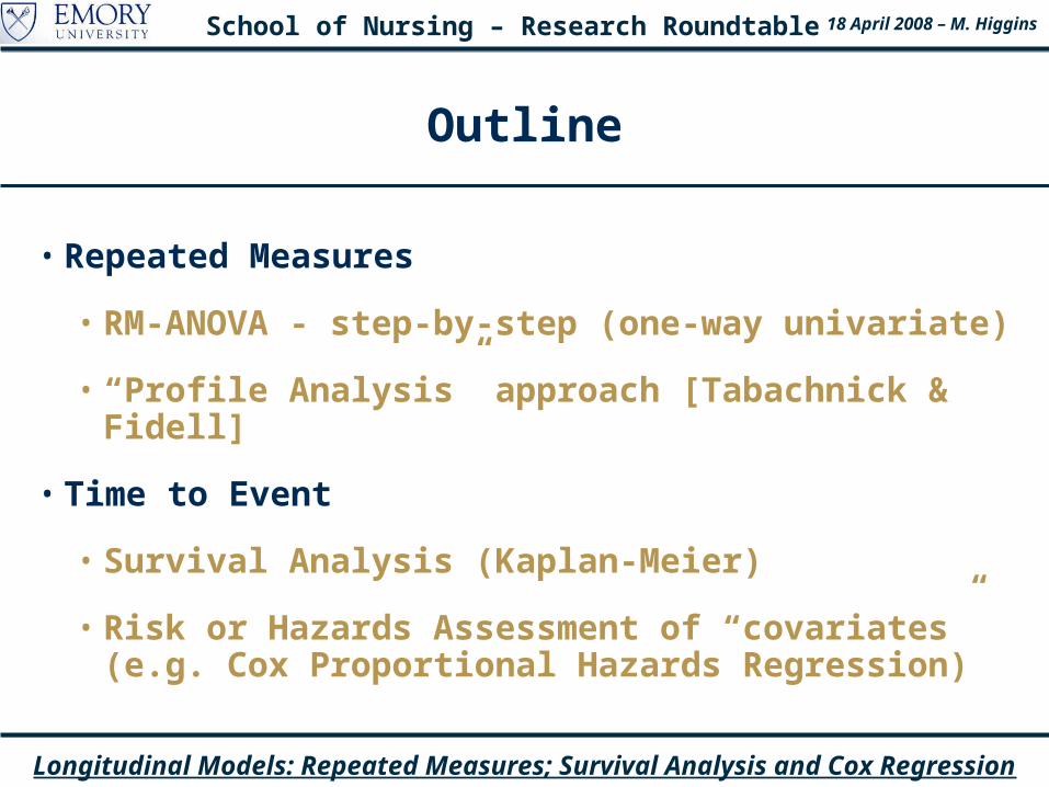
Outline

• Repeated Measures

• RM-ANOVA - step-by-step (one-way univariate)

• “Profile Analysis” approach [Tabachnick & Fidell]

• Time to Event

• Survival Analysis (Kaplan-Meier)

• Risk or Hazards Assessment of “covariates” (e.g. Cox Proportional Hazards Regression)



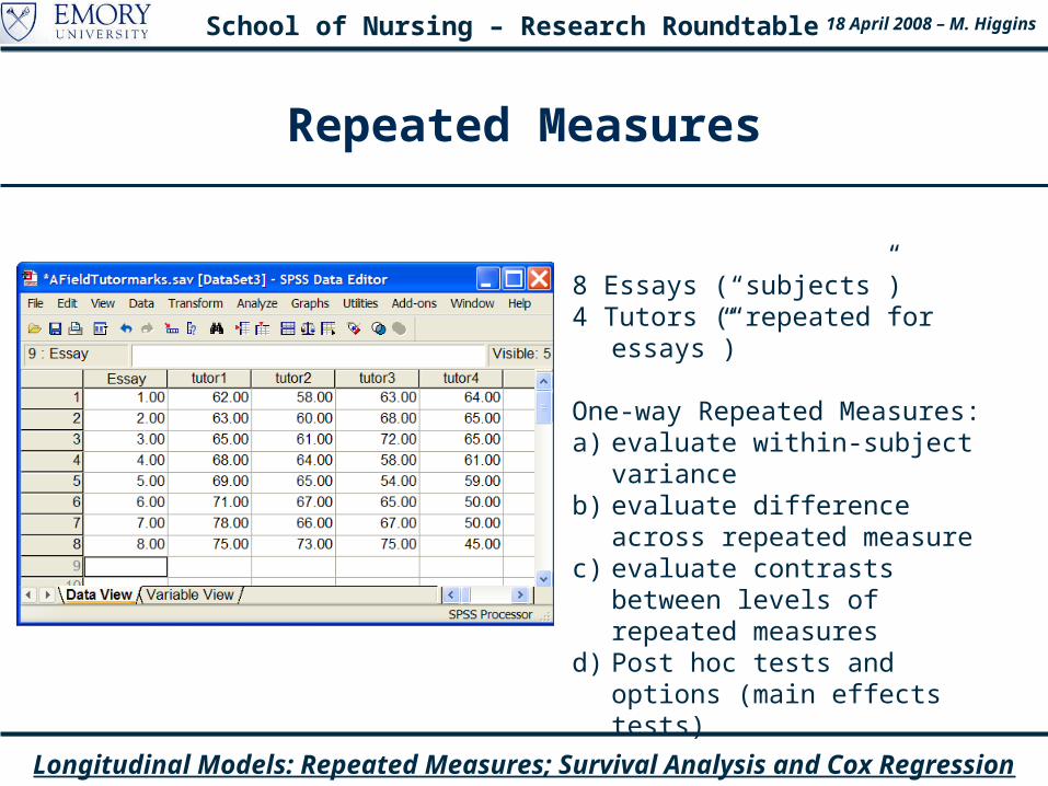
Repeated Measures

8 Essays (“subjects”)4 Tutors (“repeated for essays”)

One-way Repeated Measures:a) evaluate within-subject varianceb) evaluate difference across

repeated measurec) evaluate contrasts between levels

of repeated measuresd) Post hoc tests and options (main

effects tests)



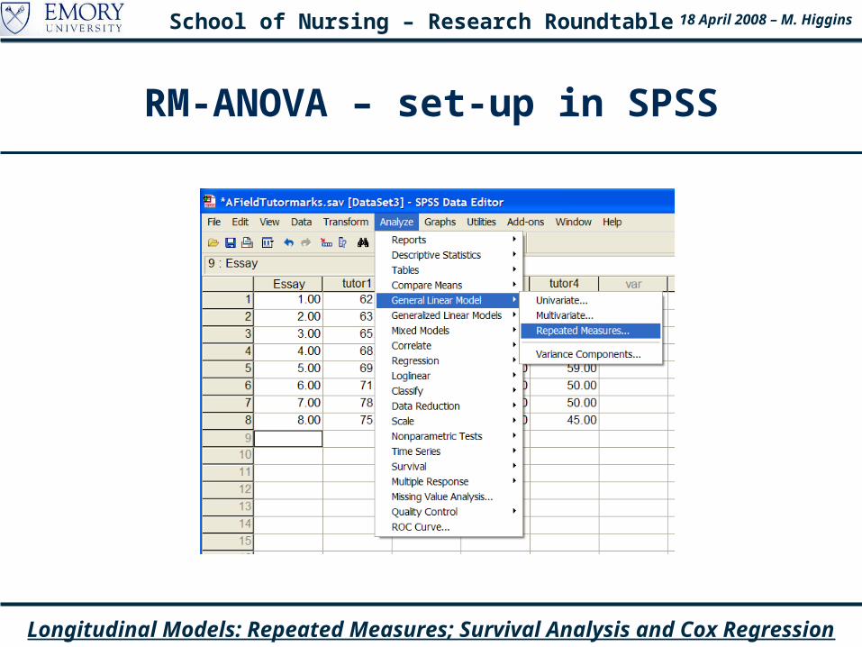
RM-ANOVA – set-up in SPSS

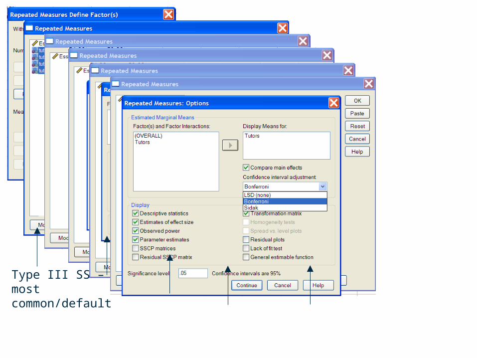
Type III SS – most common/default



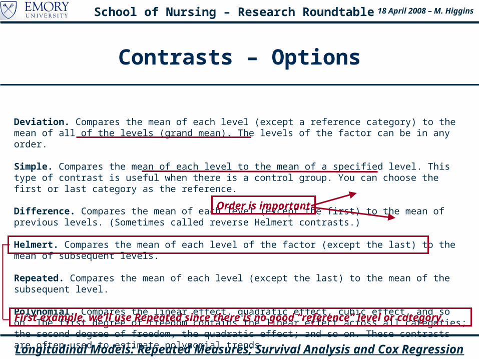
Contrasts – Options

Deviation. Compares the mean of each level (except a reference category) to the mean of all of the levels (grand mean). The levels of the factor can be in any order.

Simple. Compares the mean of each level to the mean of a specified level. This type of contrast is useful when there is a control group. You can choose the first or last category as the reference.

Difference. Compares the mean of each level (except the first) to the mean of previous levels. (Sometimes called reverse Helmert contrasts.)

Helmert. Compares the mean of each level of the factor (except the last) to the mean of subsequent levels.

Repeated. Compares the mean of each level (except the last) to the mean of the subsequent level.

Polynomial. Compares the linear effect, quadratic effect, cubic effect, and so on. The first degree of freedom contains the linear effect across all categories; the second degree of freedom, the quadratic effect; and so on. These contrasts are often used to estimate polynomial trends.

First example, we’ll use Repeated since there is no good “reference” level or category.

Order is important



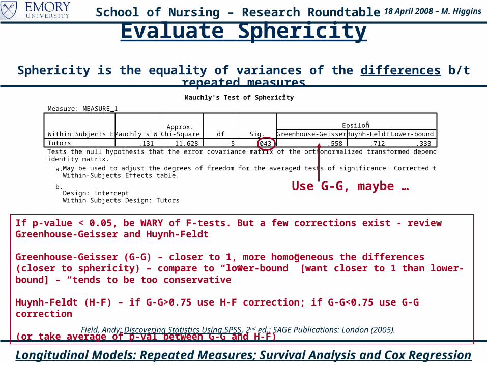
Mauchly's Test of Sphericity b

Measure: MEASURE_1

.131 11.628 5 .043 .558 .712 .333Within Subjects EffectTutors

Mauchly's WApprox.

Chi-Square df Sig. Greenhouse-Geisser Huynh-Feldt Lower-boundEpsilona

Tests the null hypothesis that the error covariance matrix of the orthonormalized transformed dependent variables is proportional to anidentity matrix.

May be used to adjust the degrees of freedom for the averaged tests of significance. Corrected tests are displayed in the Tests ofWithin-Subjects Effects table.

a.

Design: Intercept Within Subjects Design: Tutors

b.

Evaluate Sphericity

Sphericity is the equality of variances of the differences b/t repeated measures

If p-value < 0.05, be WARY of F-tests. But a few corrections exist - review Greenhouse-Geisser and Huynh-Feldt

Greenhouse-Geisser (G-G) – closer to 1, more homogeneous the differences (closer to sphericity) – compare to “lower-bound” [want closer to 1 than lower-bound] – “tends to be too conservative”

Huynh-Feldt (H-F) – if G-G>0.75 use H-F correction; if G-G<0.75 use G-G correction

(or take average of p-val between G-G and H-F)

Field, Andy; Discovering Statistics Using SPSS, 2nd ed.; SAGE Publications: London (2005).

Use G-G, maybe …



Main Repeated Measures Effects(Tests of Within-Subjects)

Tests of Within-Subjects Effects

Measure: MEASURE_1

554.125 3 184.708 3.700 .028 .346 11.100 .722554.125 1.673 331.245 3.700 .063 .346 6.189 .522554.125 2.137 259.329 3.700 .047 .346 7.906 .603554.125 1.000 554.125 3.700 .096 .346 3.700 .383

1048.375 21 49.9231048.375 11.710 89.5281048.375 14.957 70.0911048.375 7.000 149.768

Sphericity AssumedGreenhouse-GeisserHuynh-FeldtLower-boundSphericity AssumedGreenhouse-GeisserHuynh-FeldtLower-bound

SourceTutors

Error(Tutors)

Type III Sumof Squares df Mean Square F Sig.

Partial EtaSquared

Noncent.Parameter

ObservedPowera

Computed using alpha = .05a.

Sphericity was violated, and the G-G correction was indicated, although it can “tend to be too conservative.

G-G indicates we should not reject Ho: no difference across within-subjects (between the tutors).

But the H-F is significant and indicates we should reject Ho.

A. Field suggest taking the average to get a p-val = (.063+.047)/2 = .055, do not reject Ho.



Also check Multivariate Tests

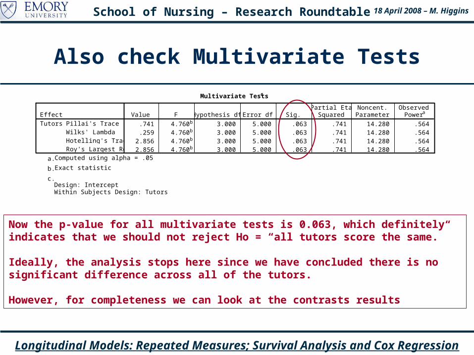
Multivariate Testsc

.741 4.760b 3.000 5.000 .063 .741 14.280 .564

.259 4.760b 3.000 5.000 .063 .741 14.280 .5642.856 4.760b 3.000 5.000 .063 .741 14.280 .5642.856 4.760b 3.000 5.000 .063 .741 14.280 .564

Pillai's TraceWilks' LambdaHotelling's TraceRoy's Largest Root

EffectTutors

Value F Hypothesis df Error df Sig.Partial EtaSquared

Noncent.Parameter

ObservedPowera


Exact statisticb.

Design: Intercept Within Subjects Design: Tutors

c.

Now the p-value for all multivariate tests is 0.063, which definitely indicates that we should not reject Ho = “all tutors score the same.”

Ideally, the analysis stops here since we have concluded there is no significant difference across all of the tutors.

However, for completeness we can look at the contrasts results



Contrasts

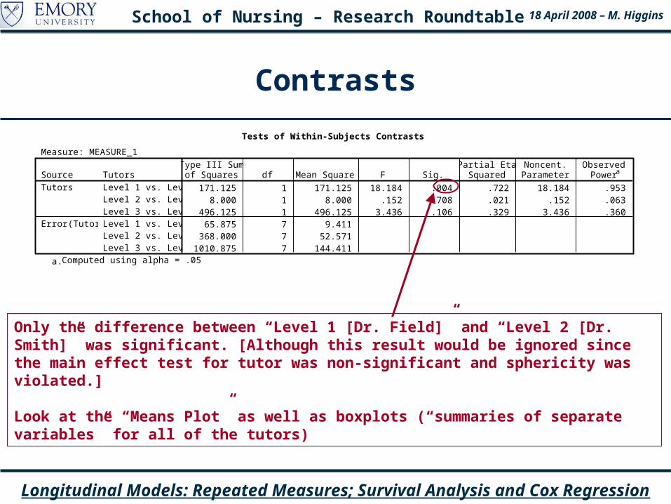
Tests of Within-Subjects Contrasts

Measure: MEASURE_1

171.125 1 171.125 18.184 .004 .722 18.184 .9538.000 1 8.000 .152 .708 .021 .152 .063

496.125 1 496.125 3.436 .106 .329 3.436 .36065.875 7 9.411

368.000 7 52.5711010.875 7 144.411

TutorsLevel 1 vs. Level 2Level 2 vs. Level 3Level 3 vs. Level 4Level 1 vs. Level 2Level 2 vs. Level 3Level 3 vs. Level 4

SourceTutors

Error(Tutors)


Partial EtaSquared

Noncent.Parameter

ObservedPowera


Only the difference between “Level 1 [Dr. Field]” and “Level 2 [Dr. Smith]” was significant. [Although this result would be ignored since the main effect test for tutor was non-significant and sphericity was violated.]

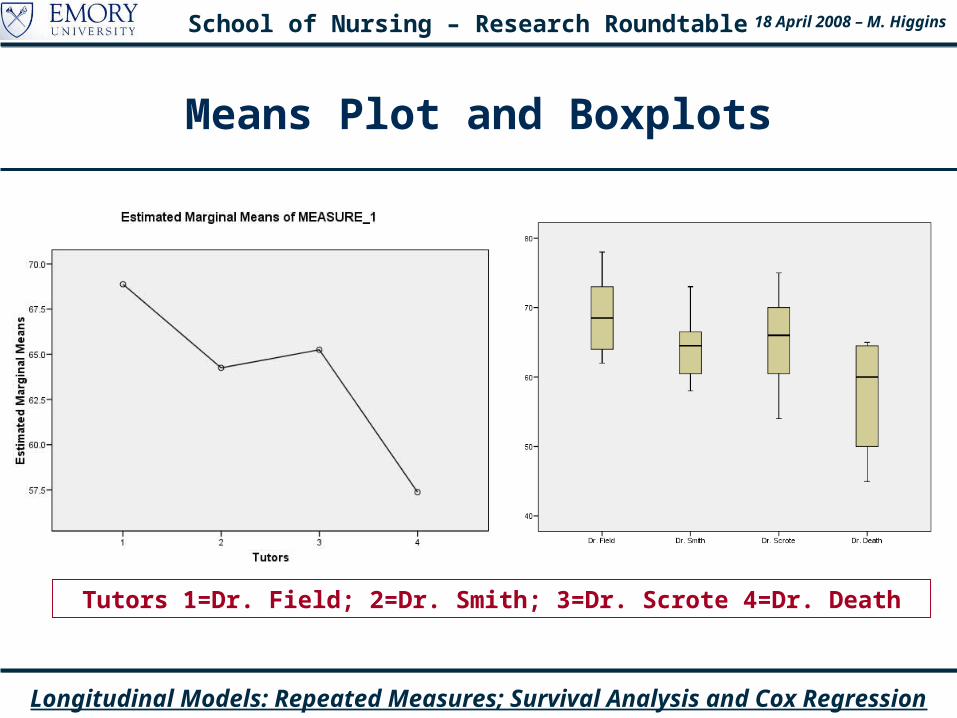
Look at the “Means Plot” as well as boxplots (“summaries of separate variables” for all of the tutors)



Means Plot and Boxplots

Tutors 1=Dr. Field; 2=Dr. Smith; 3=Dr. Scrote 4=Dr. Death



Mixed Design ANOVA (Between-groups and Repeated Measures)

Tabachnick, B. G.; Fidell, L. S. Using Multivariate Statistics (5th Ed.). Pearson Edu. Inc.: Boston, MA (2007).

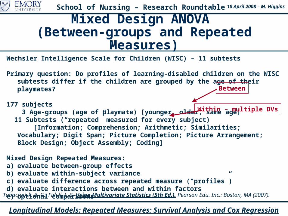
Wechsler Intelligence Scale for Children (WISC) – 11 subtests

Primary question: Do profiles of learning-disabled children on the WISC subtests differ if the children are grouped by the age of their playmates?

177 subjects 3 Age-groups (age of playmate) [younger, older, same age] 11 Subtests (“repeated” measured for every subject) [Information; Comprehension; Arithmetic; Similarities; Vocabulary; Digit Span; Picture

Completion; Picture Arrangement; Block Design; Object Assembly; Coding]

Mixed Design Repeated Measures:a) evaluate between-group effectsb) evaluate within-subject variancec) evaluate difference across repeated measure (“profiles”)d) evaluate interactions between and within factorse) optional comparisons

Between

Within – multiple DVs



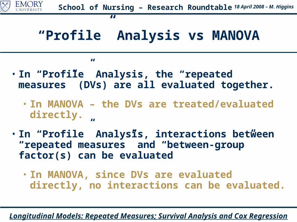
“Profile” Analysis vs MANOVA

• In “Profile” Analysis, the “repeated measures” (DVs) are all evaluated together.

• In MANOVA – the DVs are treated/evaluated directly.

• In “Profile” Analysis, interactions between “repeated measures” and “between-group” factor(s) can be evaluated

• In MANOVA, since DVs are evaluated directly, no interactions can be evaluated.



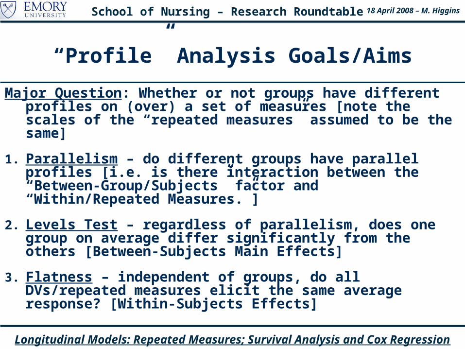
“Profile” Analysis Goals/Aims

Major Question: Whether or not groups have different profiles on (over) a set of measures [note the scales of the “repeated measures” assumed to be the same]

1. Parallelism – do different groups have parallel profiles [i.e. is there interaction between the “Between-Group/Subjects” factor and “Within/Repeated Measures.”]

2. Levels Test – regardless of parallelism, does one group on average differ significantly from the others [Between-Subjects Main Effects]

3. Flatness – independent of groups, do all DVs/repeated measures elicit the same average response? [Within-Subjects Effects]



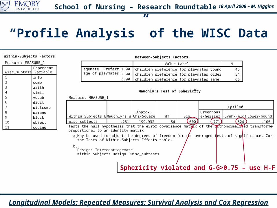
“Profile Analysis” of the WISC Data

Within-Subjects Factors

Measure: MEASURE_1

infocomparithsimilvocabdigitpictcompparangblockobjectcoding

wisc_subtests1234567891011

DependentVariable

Between-Subjects Factors

children preference for playmates younger than them 45children preference for playmates older than them 54children preference for playmates same age as them 65

1.002.003.00

agemate Preferredage of playmates

Value Label N

Mauchly's Test of Sphericity b

Measure: MEASURE_1

.281 199.932 54 .000 .771 .824 .100Within Subjects Effectwisc_subtests

Mauchly's WApprox.

Chi-Square df Sig.Greenhouse-Geisser Huynh-Feldt Lower-bound

Epsilona

Tests the null hypothesis that the error covariance matrix of the orthonormalized transformed dependent variables isproportional to an identity matrix.

May be used to adjust the degrees of freedom for the averaged tests of significance. Corrected tests are displayed inthe Tests of Within-Subjects Effects table.

a.

Design: Intercept+agemate Within Subjects Design: wisc_subtests

b.

Sphericity violated and G-G>0.75 – use H-F

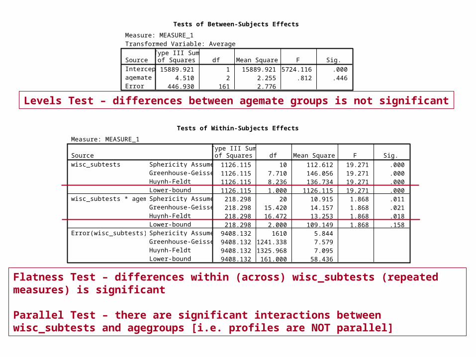
Tests of Between-Subjects Effects

Measure: MEASURE_1Transformed Variable: Average

15889.921 1 15889.921 5724.116 .0004.510 2 2.255 .812 .446

446.930 161 2.776

SourceInterceptagemateError


Levels Test – differences between agemate groups is not significant

Tests of Within-Subjects Effects

Measure: MEASURE_1

1126.115 10 112.612 19.271 .0001126.115 7.710 146.056 19.271 .0001126.115 8.236 136.734 19.271 .0001126.115 1.000 1126.115 19.271 .000218.298 20 10.915 1.868 .011218.298 15.420 14.157 1.868 .021218.298 16.472 13.253 1.868 .018218.298 2.000 109.149 1.868 .158

9408.132 1610 5.8449408.132 1241.338 7.5799408.132 1325.968 7.0959408.132 161.000 58.436

Sphericity AssumedGreenhouse-GeisserHuynh-FeldtLower-boundSphericity AssumedGreenhouse-GeisserHuynh-FeldtLower-boundSphericity AssumedGreenhouse-GeisserHuynh-FeldtLower-bound

Sourcewisc_subtests

wisc_subtests * agemate

Error(wisc_subtests)


Flatness Test – differences within (across) wisc_subtests (repeated measures) is significant

Parallel Test – there are significant interactions between wisc_subtests and agegroups [i.e. profiles are NOT parallel]



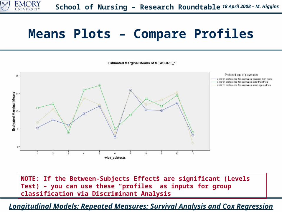
Means Plots – Compare Profiles

NOTE: If the Between-Subjects Effects are significant (Levels Test) – you can use these “profiles” as inputs for group classification via Discriminant Analysis



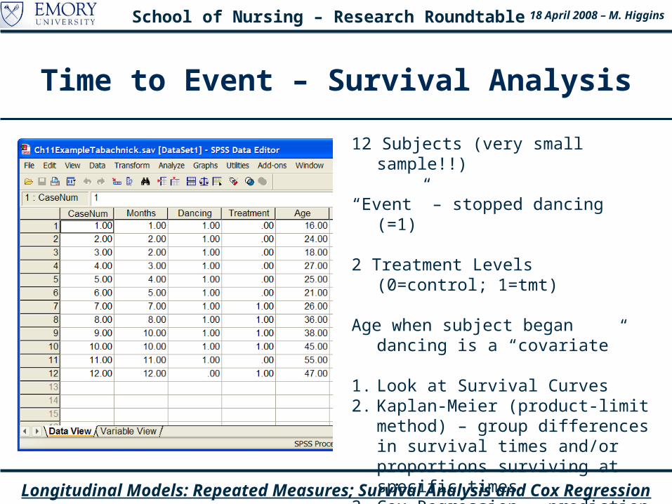
Time to Event – Survival Analysis

12 Subjects (very small sample!!)

“Event” – stopped dancing (=1)

2 Treatment Levels (0=control; 1=tmt)

Age when subject began dancing is a “covariate”

1. Look at Survival Curves2. Kaplan-Meier (product-limit method)

– group differences in survival times and/or proportions surviving at specific times

3. Cox Regression – prediction survival times from covariates

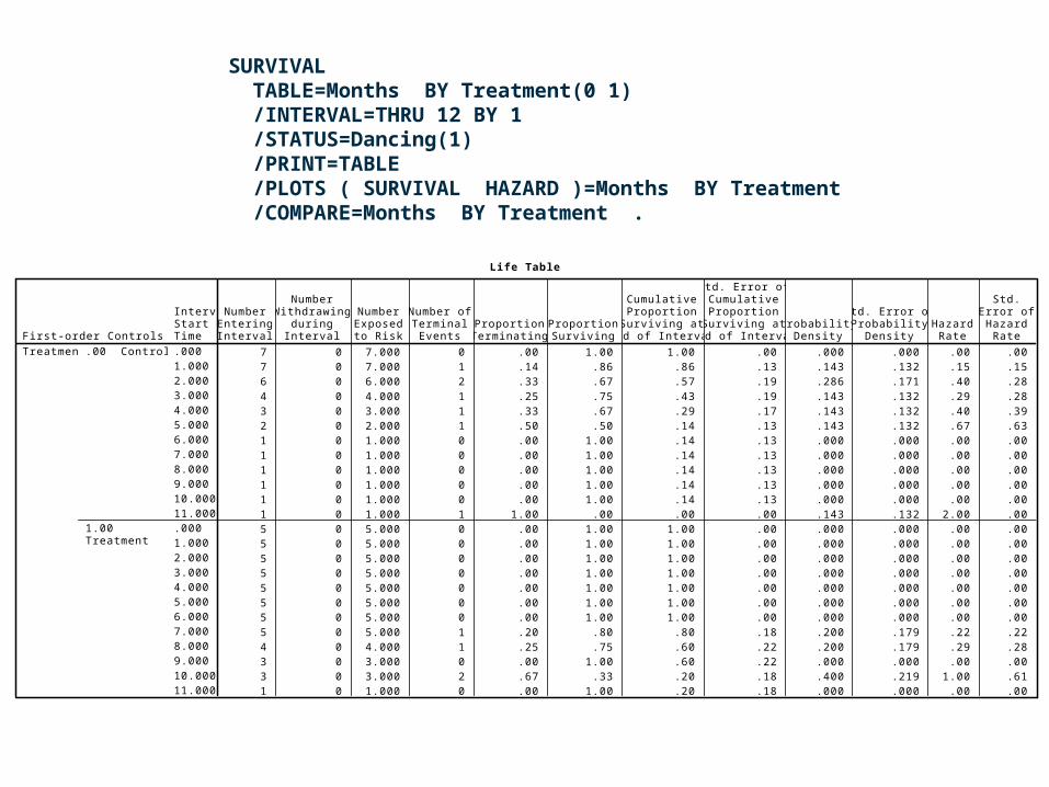
Life Table

7 0 7.000 0 .00 1.00 1.00 .00 .000 .000 .00 .007 0 7.000 1 .14 .86 .86 .13 .143 .132 .15 .156 0 6.000 2 .33 .67 .57 .19 .286 .171 .40 .284 0 4.000 1 .25 .75 .43 .19 .143 .132 .29 .283 0 3.000 1 .33 .67 .29 .17 .143 .132 .40 .392 0 2.000 1 .50 .50 .14 .13 .143 .132 .67 .631 0 1.000 0 .00 1.00 .14 .13 .000 .000 .00 .001 0 1.000 0 .00 1.00 .14 .13 .000 .000 .00 .001 0 1.000 0 .00 1.00 .14 .13 .000 .000 .00 .001 0 1.000 0 .00 1.00 .14 .13 .000 .000 .00 .001 0 1.000 0 .00 1.00 .14 .13 .000 .000 .00 .001 0 1.000 1 1.00 .00 .00 .00 .143 .132 2.00 .005 0 5.000 0 .00 1.00 1.00 .00 .000 .000 .00 .005 0 5.000 0 .00 1.00 1.00 .00 .000 .000 .00 .005 0 5.000 0 .00 1.00 1.00 .00 .000 .000 .00 .005 0 5.000 0 .00 1.00 1.00 .00 .000 .000 .00 .005 0 5.000 0 .00 1.00 1.00 .00 .000 .000 .00 .005 0 5.000 0 .00 1.00 1.00 .00 .000 .000 .00 .005 0 5.000 0 .00 1.00 1.00 .00 .000 .000 .00 .005 0 5.000 1 .20 .80 .80 .18 .200 .179 .22 .224 0 4.000 1 .25 .75 .60 .22 .200 .179 .29 .283 0 3.000 0 .00 1.00 .60 .22 .000 .000 .00 .003 0 3.000 2 .67 .33 .20 .18 .400 .219 1.00 .611 0 1.000 0 .00 1.00 .20 .18 .000 .000 .00 .00

IntervalStartTime.0001.0002.0003.0004.0005.0006.0007.0008.0009.00010.00011.000.0001.0002.0003.0004.0005.0006.0007.0008.0009.00010.00011.000

First-order Controls.00 Control

1.00 Treatment

Treatment

NumberEnteringInterval

NumberWithdrawing

duringInterval

NumberExposedto Risk

Number ofTerminalEvents

ProportionTerminating

ProportionSurviving

CumulativeProportion

Surviving atEnd of Interval

Std. Error ofCumulativeProportion

Surviving atEnd of Interval

ProbabilityDensity

Std. Error ofProbability

DensityHazard

Rate

Std.Error ofHazard

Rate

SURVIVAL TABLE=Months BY Treatment(0 1) /INTERVAL=THRU 12 BY 1 /STATUS=Dancing(1) /PRINT=TABLE /PLOTS ( SURVIVAL HAZARD )=Months BY Treatment /COMPARE=Months BY Treatment .

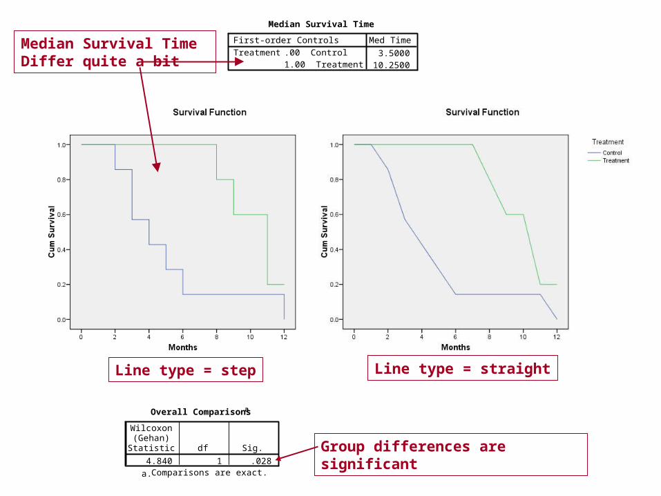
Median Survival Time

3.500010.2500

First-order Controls.00 Control1.00 Treatment

TreatmentMed Time

Line type = step Line type = straight

Overall Comparisonsa

4.840 1 .028

Wilcoxon(Gehan)Statistic df Sig.

Comparisons are exact.a.

Median Survival Time Differ quite a bit

Group differences are significant



Kaplan-MeierGroup Differences Tested via 2

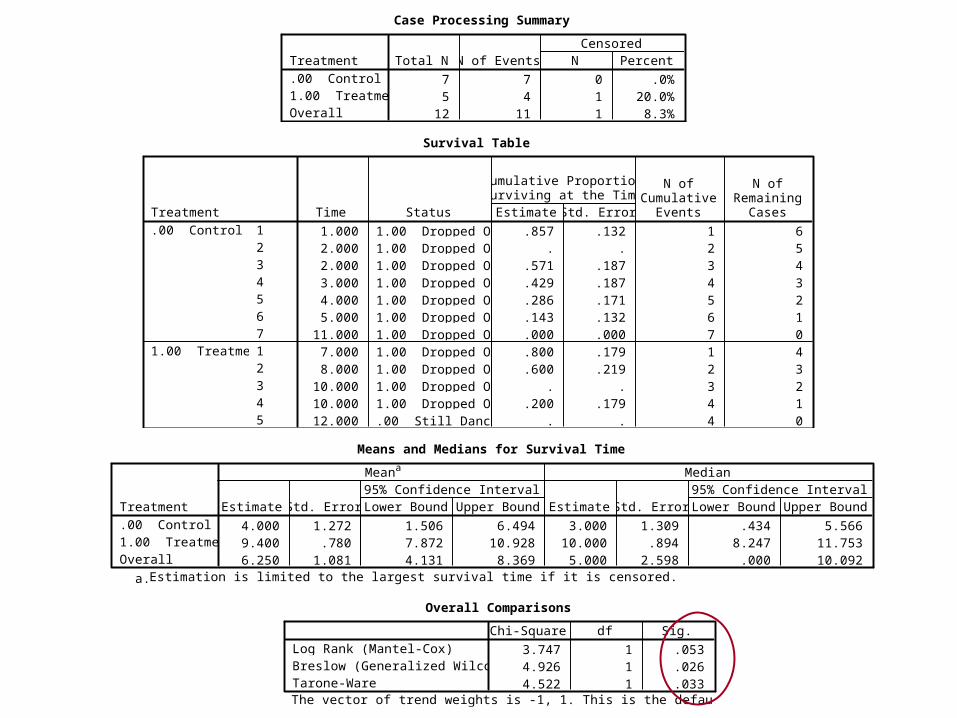
Case Processing Summary

7 7 0 .0%5 4 1 20.0%

12 11 1 8.3%

Treatment.00 Control1.00 TreatmentOverall

Total N N of Events N PercentCensored

Survival Table

1.000 1.00 Dropped Out .857 .132 1 62.000 1.00 Dropped Out . . 2 52.000 1.00 Dropped Out .571 .187 3 43.000 1.00 Dropped Out .429 .187 4 34.000 1.00 Dropped Out .286 .171 5 25.000 1.00 Dropped Out .143 .132 6 1

11.000 1.00 Dropped Out .000 .000 7 07.000 1.00 Dropped Out .800 .179 1 48.000 1.00 Dropped Out .600 .219 2 3

10.000 1.00 Dropped Out . . 3 210.000 1.00 Dropped Out .200 .179 4 112.000 .00 Still Dancing . . 4 0

123456712345

Treatment.00 Control

1.00 Treatment

Time Status Estimate Std. Error

Cumulative ProportionSurviving at the Time

N ofCumulative

Events

N ofRemaining

Cases

Means and Medians for Survival Time

4.000 1.272 1.506 6.494 3.000 1.309 .434 5.5669.400 .780 7.872 10.928 10.000 .894 8.247 11.7536.250 1.081 4.131 8.369 5.000 2.598 .000 10.092

Treatment.00 Control1.00 TreatmentOverall

Estimate Std. Error Lower Bound Upper Bound95% Confidence Interval

Estimate Std. Error Lower Bound Upper Bound95% Confidence Interval

Meana Median

Estimation is limited to the largest survival time if it is censored.a.

Overall Comparisons

3.747 1 .0534.926 1 .0264.522 1 .033

Log Rank (Mantel-Cox)Breslow (Generalized Wilcoxon)Tarone-Ware

Chi-Square df Sig.

The vector of trend weights is -1, 1. This is the default.



Cox Regression

• Cox Proportional-Hazards Regression Model – models event rates as a log-linear function of predictors (called “covariates”).

• The regression coefficients give the relative effect (or risk) of each “covariate” on the survivor function.

• NOTE: “Covariates” are both the usual covariates, but also include independent predictors and group variables (treatment)

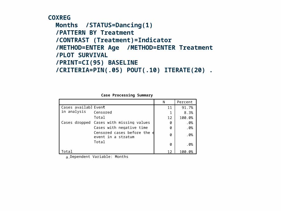
Case Processing Summary

11 91.7%1 8.3%

12 100.0%0 .0%0 .0%

0 .0%

0 .0%

12 100.0%

Eventa

CensoredTotal

Cases availablein analysis

Cases with missing valuesCases with negative timeCensored cases before the earliestevent in a stratumTotal

Cases dropped

Total

N Percent

Dependent Variable: Monthsa.

COXREG Months /STATUS=Dancing(1) /PATTERN BY Treatment /CONTRAST (Treatment)=Indicator /METHOD=ENTER Age /METHOD=ENTER Treatment /PLOT SURVIVAL /PRINT=CI(95) BASELINE /CRITERIA=PIN(.05) POUT(.10) ITERATE(20) .

Block 1: Method = EnterOmnibus Tests of Model Coefficients a,b

25.395 11.185 1 .001 15.345 1 .000 15.345 1 .000

-2 LogLikelihood Chi-square df Sig.

Overall (score)Chi-square df Sig.

Change From Previous StepChi-square df Sig.

Change From Previous Block

Beginning Block Number 0, initial Log Likelihood function: -2 Log likelihood: 40.740a.

Beginning Block Number 1. Method = Enterb.

Variables in the Equation

-.199 .072 7.640 1 .006 .819 .711 .944AgeB SE Wald df Sig. Exp(B) Lower Upper

95.0% CI for Exp(B)

Block 2: Method = EnterOmnibus Tests of Model Coefficients a,b

21.417 14.706 2 .001 3.978 1 .046 3.978 1 .046

-2 LogLikelihood Chi-square df Sig.

Overall (score)Chi-square df Sig.

Change From Previous StepChi-square df Sig.

Change From Previous Block

Beginning Block Number 0, initial Log Likelihood function: -2 Log likelihood: 40.740a.

Beginning Block Number 2. Method = Enterb.

Variables in the Equation

-.230 .089 6.605 1 .010 .795 .667 .9472.542 1.546 2.701 1 .100 12.699 .613 263.064

AgeTreatment

B SE Wald df Sig. Exp(B) Lower Upper95.0% CI for Exp(B)

Age is a significant covariate (via both Wald and -2 Log Likelihood)

Age still a significant covariate (Wald)But treatment is not (according to Wald which is better for smaller sample sizes)

Exp(B) = “odds ratio/hazard ratio”



VIII. Statistical Resources and Contact InfoSON S:\Shared\Statistics_MKHiggins

Shared resource for all of SON – faculty and students

Will continually update with tip sheets (for SPSS, SAS, and other software), lectures (PPTs and handouts), datasets, other resources and references

Statistics At Nursing Website: [moving to main website] S:\Shared\Statistics_MKHiggins\website2\index.htm

And Blackboard Site (in development) for “Organization: Statistics at School of Nursing”

Contact

Dr. Melinda Higgins

[email protected]

Office: 404-727-5180 / Mobile: 404-434-1785

Documents

18 April 2008 – M. Higgins School of Nursing – Research Roundtable Longitudinal Models: Repeated Measures; Survival Analysis and Cox Regression “Longitudinal