Embed Size (px)
Citation preview

18-661 Introduction to Machine Learning
Ensemble Methods
Spring 2020
ECE – Carnegie Mellon University

Admin
• No recitation this Friday (mid-semester break)
• Homework 4 will be released Friday, due on 3/18 (Wednesday after
spring break)
• Midterm exam grades were released yesterday. Solutions have been
posted on Canvas, and regrades will open for one week after this
lecture.
1

Outline
1. Recap: Decision Trees
2. Ensemble Methods: Motivation
3. Bagging and Random Forests
4. Boosting and AdaBoost
2

Recap: Decision Trees

Need interpretable decision boundaries
x1 x 2
• Should be able to explain the reasoning in clear terms, e.g. “I always
recommend treatment 1 when a patient has fever ≥ 100F”
• The rules that you use to make decisions can be easily used by a
lay-person without performing complex computations
• Decision trees can provide such simple decision rules
3

Many decisions are tree structured
Medical treatment
Fever
𝑇 > 100 𝑇 < 100
Treatment #1 Muscle Pain
Treatment #2
High
Treatment #3
Low
Salary in a company
Degree
High School College Graduate
Work Experience Work Experience Work Experience
< 5yr > 5yr
$𝑿𝟏 $𝑿𝟐
< 5yr > 5yr
$𝑿𝟑 $𝑿𝟒
< 5yr > 5yr
$𝑿𝟓 $𝑿𝟔
4

Special Names for Nodes in a Tree
Node
Root
Edge
Leaf
5

A tree partitions the feature space
A
B
C D
E
θ1 θ4
θ2
θ3
x1
x2
x1 > θ1
x2 > θ3
x1 6 θ4
x2 6 θ2
A B C D E
6

Learning a tree model
x1 > θ1
x2 > θ3
x1 6 θ4
x2 6 θ2
A B C D E
Three things to learn:
1. The structure of the tree.
2. The threshold values (θi ).
3. The values for the leafs
(A,B, . . .).
7

Example: Choosing whether you want to wait at a restaurant
Use the attributes to decide whether to wait (T) or not wait (F)
8
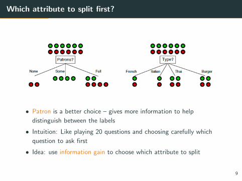
Which attribute to split first?
• Patron is a better choice – gives more information to help
distinguish between the labels
• Intuition: Like playing 20 questions and choosing carefully which
question to ask first
• Idea: use information gain to choose which attribute to split
9

Formalizing the information gain
Definition (Entropy)
If a random variable Y takes K values, a1, a2...aK , its entropy is
H[Y ] = −K∑i=1
Pr(Y = ai ) log Pr(Y = ai )
Definition (Conditional Entropy)
Given two random variables X and Y
H[Y |X ] =∑k
P(X = ak)H[Y |X = ak ]
Definition (Information Gain)
I (X ;Y ) = H[Y ]− H[Y |X ]
Measures the reduction in entropy (i.e., the reduction of uncertainty in
Y ) when we also consider X .10

Splitting on “Patron” or “Type”?
• Information gain from “Patron” is 0.55 bits.
• Information gain from “Type” is 0 bits.
Thus, we should split on “Patron” and not “Type” (higher information
gain). This is consistent with our intuition.
11

What is the optimal Tree Depth?
• What happens if we pick the wrong depth?
• If the tree is too deep, we can overfit
• If the tree is too shallow, we underfit
• Max depth is a hyperparameter that should be tuned by the data
• Alternative strategy is to create a very deep tree, and then to prune
it (see Section 9.2.2 in ESL for details)
12

How to classify with a pruned decision tree?
• If we stop here, not all training samples would be classified correctly
• More importantly, how do we classify a new instance?
• We label the leaves of this smaller tree with the majority of training
sample’s labels.
13
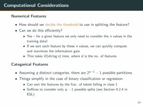
Computational Considerations
Numerical Features
• How should we decide the threshold to use in splitting the feature?
• Can we do this efficiently?
• Yes – for a given feature we only need to consider the n values in the
training data!
• If we sort each feature by these n values, we can quickly compute
and maximize the information gain
• This takes O(dn log n) time, where d is the no. of features
Categorical Features
• Assuming q distinct categories, there are 2q−1 − 1 possible partitions
• Things simplify in the case of binary classification or regression
• Can sort the features by the frac. of labels falling in class 1
• Suffices to consider only q − 1 possible splits (see Section 9.2.4 in
ESL)
14

Avoiding Overfitting in Decision Trees
Overfitting in Decision Trees
• Irrelevant attributes can result in overfitting the training example
data.
• If we have too little training data, even a reasonable hypothesis
space will overfit.
How can we avoid overfitting?
• Acquire more training data.
• Remove irrelevant attributes (manual process — not always
possible).
• Stop growing when data split is not statistically significant.
• Grow full tree, then post-prune
15

Summary of Decision Trees
Advantages of decision trees
• Can be interpreted by humans (as long as the tree is not too big)
• Handles both numerical and categorical data
• Compact representation: unlike Nearest Neighbors we don’t need
training data at test time
• But, like NN, decision trees are nonparametric because the number
of parameters depends on the data
• Building block for various ensemble methods (more on this later)
Disadvantages of decision trees
• Binary decision trees find it hard to learn linear boundaries.
• Decision trees can have high variance.
• We use heuristic training techniques: finding the optimal tree is
NP-hard.16

Ensemble Methods: Motivation

Motivation: Fighting the bias-variance tradeoff
• Simple (a.k.a weak) learners such as Naive Bayes, logistic regression,
decision stumps (shallow decision trees)
• Pros: Low variance, don’t overfit
• Cons: High Bias, can’t fit complex boundaries
Can we improve weak learners?
Idea: Train several weak learners and take an average or majority vote of
their outputs
17
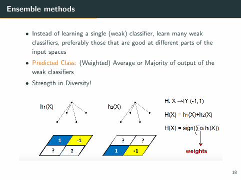
Ensemble methods
• Instead of learning a single (weak) classifier, learn many weak
classifiers, preferably those that are good at different parts of the
input spaces
• Predicted Class: (Weighted) Average or Majority of output of the
weak classifiers
• Strength in Diversity!
18

Ensemble methods
In this lecture, we will cover the following ensemble methods:
• Bagging or Bootstrap Aggregation
• Random Forests
• AdaBoost
19

Bagging and Random Forests

Bagging or Bootstrap Aggregating
To avoid overfitting a decision tree to a given dataset we can average an
ensemble of trees learnt on random subsets of the training data.
Bagging Trees (Training Phase)
• For b = 1, 2, · · · ,B• Choose n training samples (xi , yi ) from D uniformly at random
• Learn a decision tree hb on these n samples
• Store the B decision trees h1, h2, . . . hB
• Optimal B (typically in 1000s) chosen using cross-validation
Bagging Trees (Test Phase)
• For a test unlabeled example x
• Find the decision from each of the B trees
• Assign the majority label as the label for x
20

Bagging: Example
• We get different splits and thresholds for different trees b
• Predict the label assigned by majority of the B trees
• Reduces variance without increasing bias, thus avoiding overfitting21

Random Forests
• Limitation of Bagging: If one or more features are very informative,
they will be selected by almost every tree in the bag, reducing the
diversity (and potentially increasing the bias).
• Key Idea behind Random Forests: Reduces correlation between trees
in the bag without increasing variance too much
• Same as bagging in terms of sampling training data
• Before each split, select m ≤ d features at random as candidates for
splitting m ∼√d
• Take majority vote of B such trees
22

Random Forests
Increasing m, the number of splitting candidates chosen increases the
correlation among the trees in the bag 23

Random Forests
Increasing m decreases the bias but increases variance in the ensemble
24

Random Forests
25

Outline
1. Recap: Decision Trees
2. Ensemble Methods: Motivation
3. Bagging and Random Forests
4. Boosting and AdaBoost
26

Boosting and AdaBoost

Limitations of Bagging and Random Forests
• Bagging: Significant correlation between trees that are learnt on
different training datasets
• Random Forests try to resolve this by doing ”feature bagging” but
some correlation still remains
• All B trees are given the same weight when taking the average
Boosting methods: Force classifiers to learn on different parts of the
feature space, and take their weighted average
27
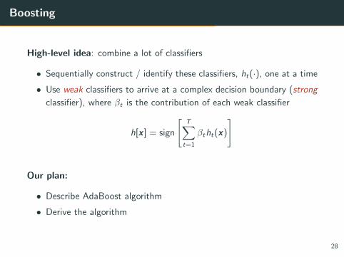
Boosting
High-level idea: combine a lot of classifiers
• Sequentially construct / identify these classifiers, ht(·), one at a time
• Use weak classifiers to arrive at a complex decision boundary (strong
classifier), where βt is the contribution of each weak classifier
h[x ] = sign
[T∑t=1
βtht(x)
]
Our plan:
• Describe AdaBoost algorithm
• Derive the algorithm
28

Adaboost algorithm
• Given: N samples {xn, yn}, where yn ∈ {+1,−1}, and some way of
constructing weak (or base) classifiers
• Initialize weights w1(n) = 1N for every training sample
• For t = 1 to T
1. Train a weak classifier ht(x) using current weights wt(n), by
minimizing
εt =∑n
wt(n)I[yn 6= ht(xn)] (the weighted classification error)
2. Compute contribution for this classifier: βt = 12
log 1−εtεt
3. Update weights on training points
wt+1(n) ∝ wt(n)e−βtynht (xn)
and normalize them such that∑
n wt+1(n) = 1
• Output the final classifier
h[x ] = sign
[T∑t=1
βtht(x)
]29

Example
10 data points and 2 featuresToy ExampleToy ExampleToy ExampleToy ExampleToy Example
D1
weak classifiers = vertical or horizontal half-planes
• The data points are clearly not linearly separable
• In the beginning, all data points have equal weights (the size of the
data markers “+” or “-”)
• Base classifier h(·): horizontal or vertical lines (’decision stumps’)
• Depth-1 decision trees, i.e., classify data based on a single attribute.
30

Round 1: t = 1
Round 1Round 1Round 1Round 1Round 1
h1
!
"11
=0.30=0.42
2D
• 3 misclassified (with circles): ε1 = 0.3→ β1 = 0.42.
• Recompute the weights; the 3 misclassified data points receive larger
weights
31
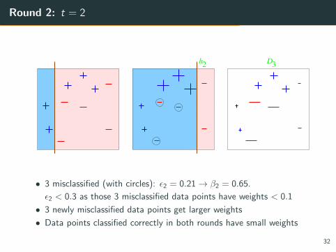
Round 2: t = 2
Round 2Round 2Round 2Round 2Round 2
!
"22
=0.21=0.65
h2 3D
• 3 misclassified (with circles): ε2 = 0.21→ β2 = 0.65.
ε2 < 0.3 as those 3 misclassified data points have weights < 0.1
• 3 newly misclassified data points get larger weights
• Data points classified correctly in both rounds have small weights
32

Round 3: t = 3
Round 3Round 3Round 3Round 3Round 3
h3
!
"33=0.92=0.14
• 3 misclassified (with circles): ε3 = 0.14→ β3 = 0.92.
• Previously correctly classified data points are now misclassified,
hence our error is low. Why?
• Since they have been consistently classified correctly, this round’s
mistake will hopefully not have a huge impact on the overall
prediction 33

Final classifier: Combining 3 classifiersFinal ClassifierFinal ClassifierFinal ClassifierFinal ClassifierFinal Classifier
Hfinal
+ 0.92+ 0.650.42sign=
=
• All data points are now classified correctly!
34

Why does AdaBoost work?
It minimizes a loss function related to classification error.
Classification loss
• Suppose we want to have a classifier
h(x) = sign[f (x)] =
{1 if f (x) > 0
−1 if f (x) < 0
• One seemingly natural loss function is 0-1 loss:
`(h(x), y) =
{0 if yf (x) > 0
1 if yf (x) < 0
Namely, the function f (x) and the target label y should have the
same sign to avoid a loss of 1.
35

Surrogate loss
0− 1 loss function `(h(x), y) is non-convex and difficult to optimize.
We can instead use a surrogate loss – what are examples?
Exponential Loss
`exp(h(x), y) = e−yf (x)
−2 0 2 4 6 8 100
1
2
3
4
5
6
7
8
yf(x)
`(h(x), y)
36

Choosing the t-th classifier
Suppose a classifier ft−1(x), and want to add a weak learner ht(x)
f (x) = ft−1(x) + βtht(x)
Note: ht(·) outputs −1 or 1, as does sign [ft−1(·)]
How can we ‘optimally’ choose ht(x) and combination coefficient βt?
Adaboost greedily minimizes the exponential loss function!
(h∗t (x), β∗t ) = argmin(ht(x),βt)
∑n
e−ynf (xn)
= argmin(ht(x),βt)
∑n
e−yn[ft−1(xn)+βtht(xn)]
= argmin(ht(x),βt)
∑n
wt(n)e−ynβtht(xn)
where we have used wt(n) as a shorthand for e−ynft−1(xn)
37

The new classifier
We can decompose the weighted loss function into two parts∑n
wt(n)e−ynβtht(xn)
=∑n
wt(n)eβt I[yn 6= ht(xn)] +∑n
wt(n)e−βt I[yn = ht(xn)]
=∑n
wt(n)eβt I[yn 6= ht(xn)] +∑n
wt(n)e−βt (1− I[yn 6= ht(xn)])
= (eβt − e−βt )∑n
wt(n)I[yn 6= ht(xn)] + e−βt
∑n
wt(n)
We have used the following properties to derive the above
• ynht(xn) is either 1 or -1 as ht(xn) is the output of a binary classifier
• The indicator function I[yn = ht(xn)] is either 0 or 1, so it equals
1− I[yn 6= ht(xn)]
38

Finding the optimal weak learner
Summary
(h∗t (x), β∗t ) = argmin(ht(x),βt)
∑n
wt(n)e−ynβtht(xn)
= argmin(ht(x),βt)(eβt − e−βt )
∑n
wt(n)I[yn 6= ht(xn)]
+ e−βt
∑n
wt(n)
What term(s) must we optimize to choose ht(xn)?
h∗t (x) = argminht(x) εt =∑n
wt(n)I[yn 6= ht(xn)]
Minimize weighted classification error as noted in step 1 of Adaboost!
39
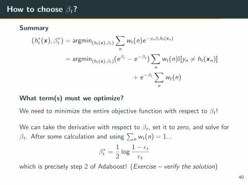
How to choose βt?
Summary
(h∗t (x), β∗t ) = argmin(ht(x),βt)
∑n
wt(n)e−ynβtht(xn)
= argmin(ht(x),βt)(eβt − e−βt )
∑n
wt(n)I[yn 6= ht(xn)]
+ e−βt
∑n
wt(n)
What term(s) must we optimize?
We need to minimize the entire objective function with respect to βt !
We can take the derivative with respect to βt , set it to zero, and solve for
βt . After some calculation and using∑
n wt(n) = 1...
β∗t =
1
2log
1− εtεt
which is precisely step 2 of Adaboost! (Exercise – verify the solution)
40

Updating the weights
Once we find the optimal weak learner we can update our classifier:
f (x) = ft−1(x) + β∗t h
∗t (x)
We then need to compute the weights for the above classifier as:
wt+1(n) ∝ e−ynf (xn) = e−yn[ft−1(x)+β∗t h
∗t (xn)]
= wt(n)e−ynβ∗t h
∗t (xn) =
{wt(n)eβ
∗t if yn 6= h∗t (xn)
wt(n)e−β∗t if yn = h∗t (xn)
Intuition Misclassified data points will get their weights increased, while
correctly classified data points will get their weight decreased
41
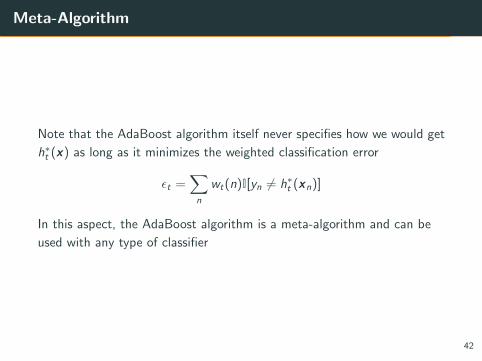
Meta-Algorithm
Note that the AdaBoost algorithm itself never specifies how we would get
h∗t (x) as long as it minimizes the weighted classification error
εt =∑n
wt(n)I[yn 6= h∗t (xn)]
In this aspect, the AdaBoost algorithm is a meta-algorithm and can be
used with any type of classifier
42

We can use decision stumps
How do we choose the decision stump classifier given the weights at the
second round of the following distribution?Round 1Round 1Round 1Round 1Round 1
h1
!
"11
=0.30=0.42
2D
We can simply enumerate all possible ways of putting vertical and
horizontal lines to separate the data points into two classes and find the
one with the smallest weighted classification error! Runtime?
• Presort data by each feature in O(dN logN) time
• Evaluate N + 1 thresholds for each feature at each round in O(dN)
time
• In total O(dN logN + dNT ) time – this efficiency is an attractive
quality of boosting!43

Other boosting algorithms
• AdaBoost is by far the most popular boosting algorithm.
• Gradient boosting generalizes AdaBoost by substituting another
(smooth) loss function for exponential loss.
• Squared loss, logistic loss, ...
• Choose the candidate learner that greedily minimizes the error
(mathematically, it should maximize the gradient of the residuals
calculated with this loss function).
• Reduce overfitting by constraining the candidate learner (e.g.,
computing the residuals only over a sample of points).
• LogitBoost minimizes the logistic loss instead of exponential loss.
• Gentle AdaBoost bounds the step size (β) of each learner update.
44

Ensemble Methods: Summary
Fight the bias-variance tradeoff by combining (by a weighted sum or
majority vote) the outputs of many weak classifiers.
Bagging trains several classifiers on random subsets of the training data.
Random forests train several decision trees that are constrained to split
on random subsets of data features.
• Prevents some correlation between trees due to dominant features.
• All classifiers are weighted equally in making the final decision.
Boosting sequentially adds weak classifiers, increasing the weight of
“hard” data points at each step.
• Greedily minimizes a surrogate classification loss
• Commonly uses decision trees as base classifiers
45