17TH NPSC, DEC 2012 1 Power System Oscillation …gopal/papers/npsc_ambientData_paper… · 17TH NPSC, DEC 2012 1 Power System Oscillation Modes Identiﬁcations: Guidelines for applying

17TH NPSC, DEC 2012 1

Power System Oscillation Modes Identifications:Guidelines for applying TLS-ESPRIT Method

Gopal Gajjar, Student-Member, IEEE, and S A Soman, Member, IEEE

Abstract—Fast measurements of power system quantities avail-able through wide area measurement systems enables directobservations of power system electromechanical oscillations. Butthe raw observations data need to be processed to obtain thequantitative measures required to make any inference regardingthe power system state. Detailed discussion is presented for thetheory behind the general problem of oscillatory mode identi-fication. This paper presents some results on oscillation modeidentification applied to a wide area frequency measurementssystem. Guidelines for selection of parameters for obtaining mostreliable results from the applied method is provided. Finally someresults on real measurements are presented with our inferenceon them.

Index Terms—Power System Oscillations, Ambient Measure-ments, TLS-ESPRIT

I. INTRODUCTION

POWER systems continuously under go changes due tostochastic nature of the loads. Each change in load also

leads to an oscillatory response from the power system. Thisis due to the dynamic nature of the power generation system.The power system oscillations are observed in most of themeasured variables like bus voltage, transmission line currents,branch powers and in the frequency as well.

With development of Wide Area Measurement Systems(WAMS) the availability of data sample at rate suitable forpower system oscillations measurement has improved. More-over the synchronized data from places separated by a distancein terms of hundreds of kilometers is available a single place.This data can be used to monitor the state of power systemby measuring observed oscillation modes.

There are several previous studies that propose methods ofextracting the system oscillation mode information form theambient power system measurements. The research in thisarea goes as far back as thirty years [1], [2]. They useda simple Discrete Fourier Transform (DFT) techniques toperform the spectral analysis and Prony and Auto correlationtechniques for mode identifications. Recent studies [3]–[7]have developed several advances signal processing methods forperforming the task of mode identification. Ref. [8] suggesteda subspace separation based technique called Total LeastSquare - Estimation of Signal Parameters through RotationalInvariant Technique TLS-ESPRIT. This method was originallyproposed for direction of arrival measurement for antennasystems [9], and it has been also applied for analysis of

Authors are with the Department of Electrical Engineering, IIT Bombay,Mumbai e-mail: [email protected], [email protected].

power quality events [10]. The major conclusion of [3], [7]is that most of the methods give comparable results undersimilar conditions. In this paper we are going to use theTLS-ESPRIT method for mode identification from ambientfrequency measurements and discuss some of the interestingfindings.

In the following sections we discuss salient features ofpower system oscillations and the wide area frequency mea-surement system which measured the input data used in thestudy. Finally some details about methodology followed inmode identifications and discuss the results obtained on thereal life data.

II. POWER SYSTEM OSCILLATIONS

In order to study the dynamic response of the power systemsa detailed multi machine analysis has to be performed asdescribed in [11], [12]. Reviewing the details of multi machineanalysis is beyond scope of this paper. But major resultsof the analysis is that any large power system will have afew dominant electromechanical modes of oscillations thatobservable in most of the system measured values. The busvoltage frequency is one of such output variable. The modesof oscillations can be broadly classified as inter area, localand intra plant modes. The inter area modes have frequencyin range of 0.2 to 0.5 Hz. and are observable in severalmeasurement outputs spread over a wide area. The local modeshave frequency range of 0.8 to 1.8 Hz. and are associated witha small group of generators oscillating against a larger system.It is observable in fewer measured values of smaller area. Theintra plant modes have higher frequency in range of 1.5 to 3 Hzand are observable only within and near by a generating plant.Over and above these there are some modes of oscillationsassociated with controls like HVDC, FACTS and turbinegovernors. Their frequency of oscillation is not fixed anddepends on the controller parameters and their observabilityin measured values depend on the power handling capacity ofthe controlled equipment and the parameter that is controlled.The controller mode of large HVDC line may be observable inwide area in active power and frequency of the system, whilea small SVC controller mode may observable in bus voltagemagnitude in its neighbourhood.

We show the method of measuring these modes of oscil-lation through a simple wide area frequency measurementsystem.

2 17TH NPSC, DEC 2012

III. WIDE AREA FREQUENCY MEASUREMENT SYSTEM

Frequency is one parameter that is measurable at every pointin a power system. Frequency measured at a low voltage levelwill also provide the measurements of the electromechanicalmodes that are observable in the high voltage bus of that area[13], [14]. Unlike phase angle measurement that require highlyaccurate clock synchronization, the frequency measurement istolerant to an error of few milli seconds in clock synchroniza-tion.

Wide Area Frequency Measurement System (WAFMS) [15]developed and deployed by Power Systems Laboratory of IITBombay, India uses Network Time Protocol (NTP) for timetagging the measured frequency. The frequency measurementdevices are placed at power outlets of several laboratories inacademic institutes spread over a synchronously connectednetwork in India. The measurements are performed locally byeach device at period of every 20 ms., and the measured datais streamed to a central server. The project is operational sincemid 2009, and at least two years of measurement archive isavailable for this study.

There are several incidents of power system oscillationsmeasured through this system, some of them are reported in[13]. The swings arising out of the large disturbances are ofgreat interest and provide important information regarding thesystem behaviour. However, the focus of this paper is more onthe power system oscillation modes that are measured duringambient conditions when there is no large event like fault,generator tripping or load shedding etc.

IV. RESPONSE OF STOCHASTIC LINEAR TIME INVARIANTSYSTEM

The previous sections discussed the typical oscillatorymodes of a power system networks and their measurements.These forms a part of a vast field of the study of lineartime invariant (LTI) systems. The properties of LTI systemsare well studied. The response of LTI system consists oftwo components. One is dependent on the forcing functionand it forms steady state component. The other componentis independent of the forcing function, but depends on theproperties of the system it self. This paper is repeating allthe well known facts of LTI system but suffice to say that thesystem response is a linear combination of damped exponentialin time. The exponential can be over-damped, without anyoscillations, or under-damped with few cycles of oscillations.These responses can be elicited from they system by giving itknown forcing function like a impulse function or a unit stepfunction.

Consider a simple continuous time single input single output(SISO) system given by

x = Ax+ Bu

y = Cx+ Du (1)(2)

where,

A =[−0.1 2π0.4−2π0.4 −0.1

]B =

[10

]C =

[1 0

]D = [0] (3)

The system has a single oscillatory mode with naturalfrequency ωn equal to 0.40032 Hz and the damping factorζ equal to 3.97 %. The natural frequency and damping factoris calculated from the complex eigen value pairs of the statematrix A as

λ = α+ jω (4)

ωn =√α2 + ω2 (5)

ζ = − α

ωn(6)

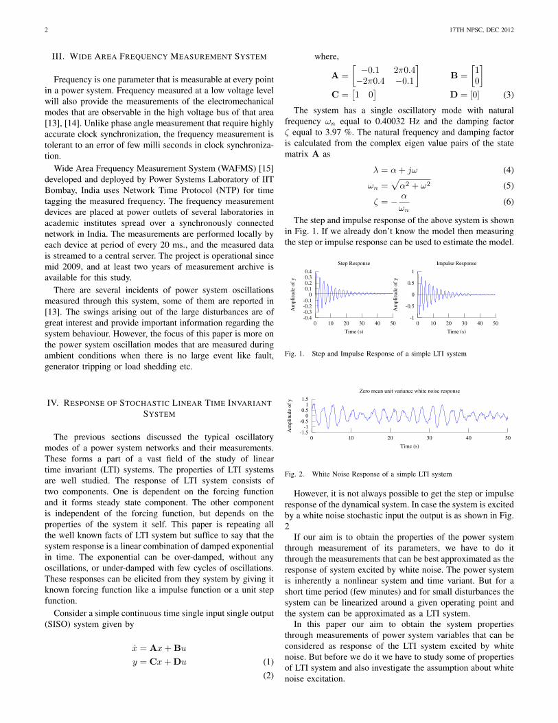
The step and impulse response of the above system is shownin Fig. 1. If we already don’t know the model then measuringthe step or impulse response can be used to estimate the model.

-0.4-0.3-0.2-0.1

00.10.20.30.4

0 10 20 30 40 50

Am

pli

tude

of

y

Time (s)

Step Response

-1

-0.5

0

0.5

1

0 10 20 30 40 50

Am

pli

tude

of

y

Time (s)

Impulse Response

Fig. 1. Step and Impulse Response of a simple LTI system

-1.5-1

-0.50

0.51

1.5

0 10 20 30 40 50

Am

pli

tude

of

y

Time (s)

Zero mean unit variance white noise response

Fig. 2. White Noise Response of a simple LTI system

However, it is not always possible to get the step or impulseresponse of the dynamical system. In case the system is excitedby a white noise stochastic input the output is as shown in Fig.2

If our aim is to obtain the properties of the power systemthrough measurement of its parameters, we have to do itthrough the measurements that can be best approximated as theresponse of system excited by white noise. The power systemis inherently a nonlinear system and time variant. But for ashort time period (few minutes) and for small disturbances thesystem can be linearized around a given operating point andthe system can be approximated as a LTI system.

In this paper our aim to obtain the system propertiesthrough measurements of power system variables that can beconsidered as response of the LTI system excited by whitenoise. But before we do it we have to study some of propertiesof LTI system and also investigate the assumption about whitenoise excitation.

GOPAL GAJJAR : SYSTEM OSCILLATION MODE IDENTIFICATION 3

A. Validity of white noise assumption

White noise is defined as a signal that has uniform powerdistribution along frequency axis in a given band. It statisticsthe white noise signal is mapped to a random variable withzero mean and constant variance [16], [17]. Any independentand identically distributed (iid) random variable satisfies theproperties of white noise. Particularly the so called normallydistributed random variable i.e. with zero mean and constantvariance Gaussian distribution is very common example of awhite noise. In this paper the white noise is always meant as aGaussian white noise. Here is should be noted that if a randomvariable is having non zero mean then the white noise signalis obtained from a Gaussian distributed random variable bysubtracting its mean value from the variable.

Power systems loads can be can be approximated by verylarge numbers of uniform loads connected by binary switches.When a switch is ON, one unit load gets connected while whenthe switch is OFF that load gets disconnected. In statisticsBinomial distribution is probability distribution of number ofsuccess X in n trials [18]. When number of trials n is largeand probability p of success of individual trial is not too near0 or 1, then the discrete Binomial distribution can be approx-imated as a continuous Gaussian distribution, due to CentralLimit Theorem. In fact [18] states that the normal (Gaussian)approximation of Binomial distributed random variable willbe quite good for values of n satisfying np(1− p) ≥ 10. Thiscondition is comfortably met in any practical power systems.The results reported by [7] also supports this assumption.

From above discussion it can be safely assumed that indeedthe LTI system representing a linearized model of powersystem at a given operating point is excited by constantlychanging load that can be approximated as a white noise fora short time. The mean value of load it self and hence theoperating point of the power system changes over period oftime.It is expected that variance of the white noise representingthe stochastic change in load will also change over a periodof time. However that time period could be in terms of tensof minutes. For a short period of few minutes the white noiseassumption can still be valid.

B. Output of LTI system when excited by white noise

We have seen the plot of the time response of the system (1)when excited by a white noise in Fig. 2. The proper analysisof LTI system excited by white noise is presented here.

The analysis becomes easy if the continuous time LTIsystem in (1) is discretized as (7).

x[n+ 1] = Adx[n] + Bdu[n] (7)y[n] = Cdx[n] + Ddu[n] (8)

Where, Ad, Bd, Cd and Dd are discretized state matrixderived from A, B, C and D respectively and the discretiza-tion time T [19].

Ad = eAT Bd =

(∫ T

0

eAτdτ

)B or A−1(Ad − I)B

Cd = C Dd = D (9)

With sampling time T of 0.1 sec, the discrete representationof example in (1) becomes,

Ad =[

0.9589 0.2462−0.2462 0.9589

]Bd =

[0.09846−0.01242

]Cd =

[1 0

]Dd = [0] (10)

And with sampling time T of 0.01 sec, the discrete repre-sentation of example in (1) becomes,

Ad =[

0.9987 0.0251−0.0251 0.9987

]Bd =

[9.994e− 3−1.256e− 4

]Cd =

[1 0

]Dd = [0] (11)

It can be seen from (9)that the values in the discretizedmatrix depends on the sampling time period used.

Using the form of (7), we now show relationship betweenthe white noise input u and the corresponding output y. It canbe shown that if A is stable and input u is zero mean anda constant variance signal than the output signal y will alsohave zero mean and its variance is derives as [20],

Xcov =∞∑k=0

AdkBdUcovBd

T(Ad

T)k

(12)

Ycov = CdXcovCdT + DdUcovDd

T (13)

Where, Ucov, Xcov and Ycov are the covariance matricesdefined as expected values,

Ucov := E{

[u[n]− µu] [u[n]− µu]T}

(14)

here µu is mean value of u, it is equal to zero and can beignored. Similar equations apply for Xcov and Ycov. The autocovariance matrix is also defined for different integer lags l.

Ucov[l] := E{u[n]u[n+ l]T

}(15)

This shows that mean of x and y are zero and their covari-ance matrix are constant hence both x and y are stationaryprocesses. This is of course subject to stability of A, whichimplies that all eigen values of A have a non positive realpart. For Ad this translate into the requirement that absolutevalues of all its eigen values are less than or equal to 1.

Finally, it can be shown that the impulse response of the LTIsystem is directly related to Ycov[l]. h[lT] is discrete valuedimpulse response of LTI system and Ycov[0] is covariance ofy with zero lag as in (13).

h[lT] =Ycov[l]Ycov[0]

(16)


C. Some important aspects of response of stochastic LTIsystems

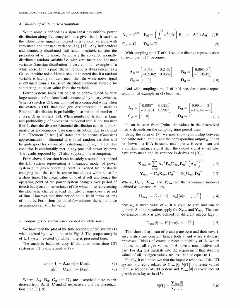
Our aim is to identify the systems or the components of thesignal from the measured signals that are response of stochas-tic LTI system. In general power systems signal the excitationapplied to the system is not in our control. However, there aresome methods that apply artificial excitation called probingsignal [21], [22]. The main aim of that signal is to excitethe system modes with enough energy that their measurementbecomes easier. In terms of our analysis the probing signalscorresponds the white noise input u, and through extra probingsignal effort is made to increase the variance Ucov, in order toget higher variance in y. Important choice for probing signal isits bandwidth. Higher bandwidth probing signal requires fastvarying devises and possibly higher energy. Here we comparethe response of the LTI system of (1) for excitation by unitvariance u with bandwidth of 10π and 100π radians. Theoutput y is shown in Fig. 3, and plot of covariance of yobtained from output of length 150 Sec is shown in Fig. 4.It can be seen that it resembles quite nearly to the impulseresponse of the system shown in Fig. 1, except for the scalingfactor. It can also be seen that the frequency of oscillationis captured quite accurately, while the damping of oscillationshows some error compared to actual impulse response. This isbecause of finite time period used for estimating the covariancematrix as against the infinite time required by for calculatingexpected value as (15). Next, we see the effect of damping on

-1.5

-1

-0.5

0

0.5

1

1.5

0 10 20 30 40 50

Am

pli

tude

of

y

Time (s)

Excitation BW 10π rad

-0.4

-0.3

-0.2

-0.1

0

0.1

0.2

0.3

0.4

0 10 20 30 40 50

Am

pli

tude

of

y

Time (s)

Excitation BW 100π rad

Fig. 3. LTI excited by white noise of different bandwidths

-0.3

-0.2

-0.1

0

0.1

0.2

0.3

0 5 10 15 20

Covar

iance

Time (s)

Output covariance with BW 10π rad

-0.03

-0.02

-0.01

0

0.01

0.02

0.03

0 5 10 15 20

Covar

iance

Time (s)

Output covariance with BW 100π rad

Fig. 4. Covariance for response with different bandwidths

the response of LTI excited by white noise. Here we see thatlower damping translate into higher covariance of y. Hencesystem with low damping will have lower SNR. Also it canbe proved that the covariance of y depends only on the real partof eigen value corresponding to the oscillation frequency. So,only real part α rather than the damping factor ζ is governingthe SNR and success of identification of the system. This resultis important in a way that existing literature and conventional

TABLE IOUTPUT COVARIANCE FOR VARYING λ

Case λ ωn ζ Ycov Ycov

(rad) (%) Calc. Meas.1 -0.1+j2π0.4 2.5153 3.97 0.246 0.243

2 -0.1+j2π0.04 0.2705 36.97 0.247 0.282

3 -0.01+j2π0.4 2.5133 0.40 2.484 2.097

4 -0.01+j2π0.04 0.2515 3.97 2.497 2.049

5 -0.5+j2π0.4 2.5625 19.51 0.047 0.052

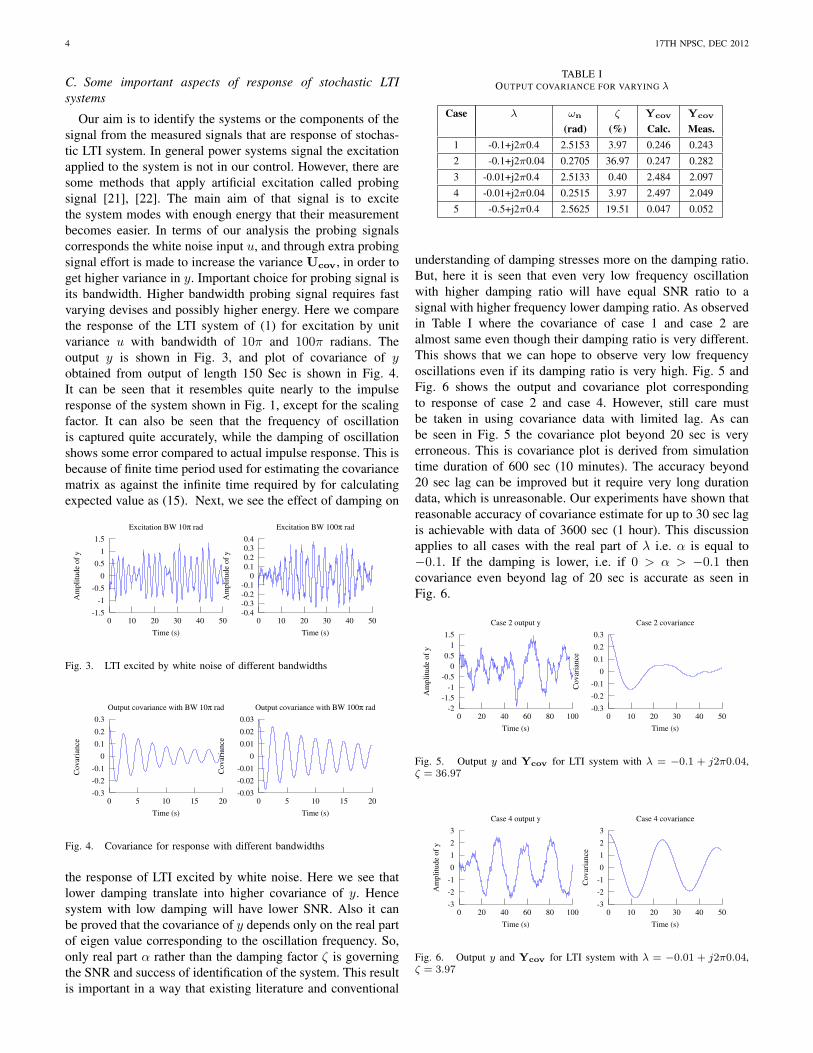
understanding of damping stresses more on the damping ratio.But, here it is seen that even very low frequency oscillationwith higher damping ratio will have equal SNR ratio to asignal with higher frequency lower damping ratio. As observedin Table I where the covariance of case 1 and case 2 arealmost same even though their damping ratio is very different.This shows that we can hope to observe very low frequencyoscillations even if its damping ratio is very high. Fig. 5 andFig. 6 shows the output and covariance plot correspondingto response of case 2 and case 4. However, still care mustbe taken in using covariance data with limited lag. As canbe seen in Fig. 5 the covariance plot beyond 20 sec is veryerroneous. This is covariance plot is derived from simulationtime duration of 600 sec (10 minutes). The accuracy beyond20 sec lag can be improved but it require very long durationdata, which is unreasonable. Our experiments have shown thatreasonable accuracy of covariance estimate for up to 30 sec lagis achievable with data of 3600 sec (1 hour). This discussionapplies to all cases with the real part of λ i.e. α is equal to−0.1. If the damping is lower, i.e. if 0 > α > −0.1 thencovariance even beyond lag of 20 sec is accurate as seen inFig. 6.

-2

-1.5

-1

-0.5

0

0.5

1

1.5

0 20 40 60 80 100

Am

pli

tude

of

y

Time (s)

Case 2 output y

-0.3

-0.2

-0.1

0

0.1

0.2

0.3

0 10 20 30 40 50

Covar

iance

Time (s)

Case 2 covariance

Fig. 5. Output y and Ycov for LTI system with λ = −0.1 + j2π0.04,ζ = 36.97

-3

-2

-1

0

1

2

3

0 20 40 60 80 100

Am

pli

tude

of

y

Time (s)

Case 4 output y

-3

-2

-1

0

1

2

3

0 10 20 30 40 50

Covar

iance

Time (s)

Case 4 covariance

Fig. 6. Output y and Ycov for LTI system with λ = −0.01 + j2π0.04,ζ = 3.97


V. METHODOLOGY

It is reasonable to assume that in ambient conditions thepower system behaves as linear time invariant system. Thesystem response can be expressed as sum of finite numbers ofdamped sinusoidal signals. Expressed as function of time

y(t) =d∑l=1

aleαlt cos(ωlt+ φl) (17)

The main aim is to identify or estimate all a, α, ω andφ from discrete measurement samples of the signal y(t). Theusual methods take the cue from the results shown in previoussection that covariance of the measured signal with sufficientlags is proportional to the impulse response of the system. Theeffect of additive measurement noise and the inherent noisedue to finite period of measurements can be mitigated fromincreasing the measurement period.

Once the auto covariance matrix is obtained with enoughaccuracy then one of the numerous methods for parametriccurve fitting can be applied to estimate the parameters of thesystem [16]. There are several methods used till now withalmost similar results, here we will use the TLS-ESPRITmethod which is shown to be one of the most accurate methodsfor spectrum estimation in [16].

Estimation of Signal Parameters Through Rotational In-variant Techniques (TLS-ESPRIT) [9] algorithm is used toestimate all a, α, ω and φ, from discrete measurement samplesof the signal y(t).

The mathematical details of TLS-ESPRIT method is pro-vided in [9], [16]. Here we discuss the application of themethod to real power system frequency signal. There areseveral parameters in the method that require proper tuning toget the reliable results. The major parameters include, ensuringthe adherence to basic assumption regarding stationarity andzero mean nature of the input signal. Next, is selection ofnumber of dominant modes, the duration of input data andthe sampling time.

A. Preprocessing

As discussed in the [13], we have a simple frequencymeter working of a zero crossing detector principle. Moreoverthe frequency meter is connected to academic laboratoriesmeasuring frequencies at 230 V power outlets.

The input data sometimes have some missing sample andalso some samples that are outliers. In the preprocessing stagewe eliminate such data points and concatenate the remainingdata. Ref. [3], as well as our own studies have confirmed thatdiscarding some small percentage of bad data does not effectthe final result.

The frequency in India varies by a large margin due toabsence of automatic secondary frequency system. This vari-ation in frequency is not due to any power system oscillationsbut a very slow (compared to usual oscillation frequencies)random drift. To ensure the stationarity and zero mean natureof the input signal this drift have to filtered out. Moreover themeasurement itself contains a high frequency measurementnoise, which is also filtered out so that it does not mask thereal oscillation frequencies.

Initially a fourth order Butterworth filter was considered forpreprocessing. The fourth order IIR Butterworth filter is veryefficient filter, but its phase response is non linear and hencedifferent frequencies in the pass bands are phase shifted bydifferent angles. Also its transition band from pass band tostop band is not very sharp. Hence another FIR filter is alsoimplemented as a substitute for Butterworth filter. This FIRfilter has linear phase response and sharper transition band.As the actual signal is measured at 50 Hz while the pass bandrequired is from 0.1 Hz to 1.5 Hz the default FIR filter isof more than 2000 order. Here we applied multistage filteringand resampling techniques [16] to overcome this high orderfiltering. The actual high pass filter to remove frequency below0.1 Hz was implemented as four stages of 5 Hz, 1 Hz, 0.2 Hzand 0.1 Hz, with first three stages of order 40 and the laststage with order 80.

B. Mode Identification

A major decision is the selection of the parameter forlength of the covariance lag and number of dominant modes.The TLS-ESPRIT algorithm decomposes the signal as linearcombination of d vectors in M dimensional subspace, whereM is length of lag of covariance. Hence, it is required thatM > d. Moreover in presence of noise, it is observed that thefrequency estimation is reliable when there is at least half acycle of the signal covered by the vector of length M . Thelowest frequency component in the input signal is 0.1 Hz,due to the lower cut off frequency of the preprocessing filter.Combined with the knowledge of sampling time of 200 msec.we get the limit of M equal to 25. Here we selected M = 100corresponding to frequency limit of 0.025 Hz. Larger valueof M is not desirable as it increases the dimension of thecovariance matrix Ycov, whose dimension is 2M × 2M . Thefirst step of the TLS-ESPRIT algorithm is to calculate 2ddominant eigen values of Ycov.

Choice of d depends on the expected number of the indepen-dent frequency components in the signal. Usually large d willbetter fit of the signal, but also give rise to spurious signals thatare mere numerical artifacts. TLS-ESPRIT method provides aneasy way to identify the spurious signals and discard themat the very beginning. The idea of subspace separation isthat the signal subspace is dominant over the noise subspace.There are only few singular values of Y corresponding thesignal subspace with dimension 2d. The rest of the singularvalues corresponds to the noise subspace. We use the fact thatvector norm of set of all eigen values of a matrix is equal tothe Frobenious norm of that matrix. The dimension of signalsubspace can be identified by a criteria such that.

min p p = 1, · · · , Ns.t.√√√√ p∑k=1

σ2k ≥ κ||Y||F (18)

Where σk are singular values of Y. κ is parameter for con-trolling how many signal components are considered. Usuallyvalue of κ is kept larger than 0.9. p separates out the dominant


signal subspace created by the range of the first p vectors of V.The subspace spanned by rest of the vectors of V correspondsto the noise subspace. In practice we do not calculate the SVDof Y as it is numerically very costly. Instead we use limitedeigen value calculation of Ycov. Using the knowledge thateigen values of Ycov are equal to square of the singular valuesof Y, and applying (18) we can find p.

Then the usual TLS-ESPRIT algorithm is followed forcalculating the selected signals frequency ω and amplitude aare calculated. The phase angle term φ, do not make muchsense for frequency estimation from ambient signals.

C. Calculation Window

We use the time block of 600 sec, at a sample time on200 msec. for calculating the oscillatory modes through TLS-ESPRIT. The available data sampled at 20 msec, is downsampled for this purpose. Use of down sampled data does notlead to any big loss of accuracy, but provides a very significantsaving in the computation time. These choices correspond toparameter h = 0.2 and M ×N ≈ 3000.

A sliding window frequency estimation is performed withthe shift of 100 seconds for each window. Hence we obtainnew frequency parameters of oscillatory modes every 100seconds using the preprocessed data of previous 600 seconds.One could select a shift of smaller value like 20 seconds ora larger value like 300 seconds, with corresponding increaseor decrease in the computation effort respectively. The choiceof shift of 100 seconds is just for convenience. The amplitudeof each mode is calculated in a batch five vectors each oflength M , corresponding the frequency data of 20 seconds. Sofive such vectors taken at consecutive time cover the slidingwindow shift of 100 seconds.

D. Mode Identification

The analysis is performed on the measured frequency sig-nals using the methodology described in the previous sec-tions. As we are interested in identification of the dominantoscillating modes from ambient frequency measurements, thesequential analysis is performed on a continuous basis. Thefrequency and the amplitudes of oscillations are compared overdifferent periods and over different locations. Some inferencesabout the state of the network is drawn through the evolutionof modes over a period of time, absence or presence ofsome modes and their magnitude. The next sections givespreliminary results and discusses their significance.

VI. RESULTS AND DISCUSSIONS

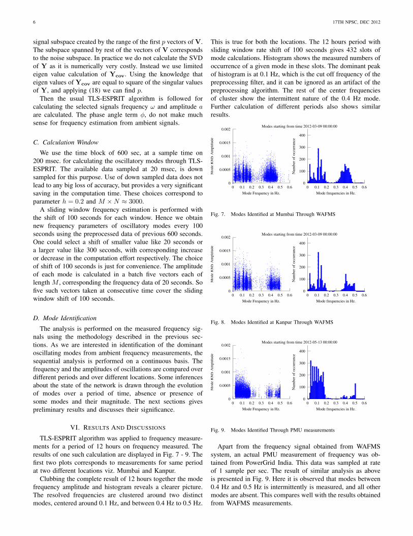
TLS-ESPRIT algorithm was applied to frequency measure-ments for a period of 12 hours on frequency measured. Theresults of one such calculation are displayed in Fig. 7 - 9. Thefirst two plots corresponds to measurements for same periodat two different locations viz. Mumbai and Kanpur.

Clubbing the complete result of 12 hours together the modefrequency amplitude and histogram reveals a clearer picture.The resolved frequencies are clustered around two distinctmodes, centered around 0.1 Hz, and between 0.4 Hz to 0.5 Hz.

This is true for both the locations. The 12 hours period withsliding window rate shift of 100 seconds gives 432 slots ofmode calculations. Histogram shows the measured numbers ofoccurrence of a given mode in these slots. The dominant peakof histogram is at 0.1 Hz, which is the cut off frequency of thepreprocessing filter, and it can be ignored as an artifact of thepreprocessing algorithm. The rest of the center frequenciesof cluster show the intermittent nature of the 0.4 Hz mode.Further calculation of different periods also shows similarresults.

0

0.0005

0.001

0.0015

0.002

0 0.1 0.2 0.3 0.4 0.5 0.6

Mode

RM

S A

mpli

tude

Mode Frequency in Hz.

0

100

200

300

400

0 0.1 0.2 0.3 0.4 0.5 0.6

Num

ber

of

occ

urr

ance

Mode frequencies in Hz.

Modes starting from time 2012-03-09 00:00:00

Fig. 7. Modes Identified at Mumbai Through WAFMS

0

0.0005

0.001

0.0015

0.002

0 0.1 0.2 0.3 0.4 0.5 0.6

Mode

RM

S A

mpli

tude


0

100

200

300

400

0 0.1 0.2 0.3 0.4 0.5 0.6N

um

ber

of

occ

urr

ance



Fig. 8. Modes Identified at Kanpur Through WAFMS

0

0.0005

0.001

0.0015

0.002

0 0.1 0.2 0.3 0.4 0.5 0.6

Mode

RM

S A

mpli

tude


0

100

200

300

400

0 0.1 0.2 0.3 0.4 0.5 0.6

Num

ber

of

occ

urr

ance



Fig. 9. Modes Identified Through PMU measurements

Apart from the frequency signal obtained from WAFMSsystem, an actual PMU measurement of frequency was ob-tained from PowerGrid India. This data was sampled at rateof 1 sample per sec. The result of similar analysis as aboveis presented in Fig. 9. Here it is observed that modes between0.4 Hz and 0.5 Hz is intermittently is measured, and all othermodes are absent. This compares well with the results obtainedfrom WAFMS measurements.


Voltage magnitude data measured from PMU is also avail-able. However it is very noisy and the analysis through TLS-ESPRIT fails to identify any dominant frequencies from thatdata. This could be the case of errors introduced due to feed-forward coupling that is locally possible in voltage data.

Out of the identified mode frequencies, the 0.4 Hz frequencyseems to be in agreement with the established theory of theinter area oscillations, which states the range of their frequencybetween 0.2 to 0.5 Hz.

A recent report [23] published by PowerGrid India, havehighlighted the observations of 0.4 Hz mode for a long timeof about 5 minutes. This was attributed to a faulty controlsystem of two 500 MW thermal generators. Power generationof the units varied from 30 MW to 250 MW and caused thismode to be excited at high amplitude. Indirectly this shows thevalidity of using probing signal to elicit the modes of system.But, the report overlooks the fact that similar oscillations of0.4 Hz but of lower magnitude were observed throughout theperiod of 12 before the said observation. Such incidents alsorequire further investigations.

VII. CONCLUSION

Identification of oscillations modes in power system throughobservation of the ambient disturbance in frequency can beachieved with a reasonable accuracy. The analysis throughLTI system response to white noise gives valuable insightsregarding the methods and expected outcome of the identifi-cation techniques. The paper demonstrates the use of TLS-ESPRIT algorithm for power system oscillation mode iden-tifications. With applications to real life data, and throughtesting with tuning of different parameters of the algorithmthe characteristics of the algorithm is judged. The TLS-ESPRIT algorithm, combined with proper preprocessing, wasfound reliable in identifying the modes of oscillations evenunder noisy measurement environment. This paper also showseffectiveness of using simple NTP based wide area frequencymeasurement system in performing quite useful analysis. Themodes revealed by the analysis of this paper give motivationfor further research in characterization of very low frequencyoscillations observed in Indian power network.

ACKNOWLEDGMENT

The authors would like to thank Prof. A M Kulkarni andhis students for WAFMS and PowerGrid India for providingan actual PMU data.

REFERENCES

[1] J. Hauer and R. Cresap, “Measurement and modeling of pacific ACintertie response to random load switching,” IEEE Transactions onPower Apparatus and Systems, vol. PAS-100, no. 1, pp. 353–359, Jan.1981.

[2] J. Pierre, D. Trudnowski, and M. Donnelly, “Initial results in electrome-chanical mode identification from ambient data,” IEEE Transactions onPower Systems, vol. 12, no. 3, pp. 1245–1251, Aug. 1997.

[3] D. Trudnowski, J. Pierre, N. Zhou, J. Hauer, and M. Parashar, “Perfor-mance of three Mode-Meter Block-Processing algorithms for automateddynamic stability assessment,” IEEE Transactions on Power Systems,vol. 23, no. 2, pp. 680–690, May 2008.

[4] G. Liu and V. Venkatasubramanian, “Oscillation monitoring from am-bient PMU measurements by frequency domain decomposition,” inCircuits and Systems, 2008. ISCAS 2008. IEEE International Symposiumon. IEEE, May 2008, pp. 2821–2824.

[5] N. Zhou, D. Trudnowski, J. Pierre, and W. Mittelstadt, “Electromechan-ical mode online estimation using regularized robust RLS methods,”IEEE Transactions on Power Systems, vol. 23, no. 4, pp. 1670–1680,Nov. 2008.

[6] D. J. Trudnowski and J. W. Pierre, “Overview of algorithms forestimating swing modes from measured responses,” in Power & EnergySociety General Meeting, 2009. PES ’09. IEEE. IEEE, Jul. 2009, pp.1–8.

[7] J. Turunen, J. Thambirajah, M. Larsson, B. C. Pal, N. F. Thornhill, L. C.Haarla, W. W. Hung, A. M. Carter, and T. Rauhala, “Comparison ofthree electromechanical oscillation damping estimation methods,” IEEETransactions on Power Systems, vol. 26, no. 4, pp. 2398–2407, Nov.2011.

[8] P. Tripathy, S. C. Srivastava, and S. N. Singh, “A modified TLS-ESPRIT-Based method for Low-Frequency mode identification in power systemsutilizing synchrophasor measurements,” IEEE Transactions on PowerSystems, vol. 26, no. 2, pp. 719–727, May 2011.

[9] R. Roy and T. Kailath, “ESPRIT-estimation of signal parameters via ro-tational invariance techniques,” IEEE Transactions on Acoustics, Speech,and Signal Processing, vol. 37, no. 7, pp. 984–995, Jul. 1989.

[10] I. Y. Gu and M. H. J. Bollen, “Estimating interharmonics by us-ing Sliding-Window ESPRIT,” IEEE Transactions on Power Delivery,vol. 23, no. 1, pp. 13–23, Jan. 2008.

[11] P. Kundur, Power System Stability And Control. New York, NY, USA:McGraw-Hill, Inc., 1994.

[12] K. R. Padyar, Power System Dynamics Stability And Control, 2nd ed.Hyderabad, AP, India: BS Publications, 2002.

[13] K. A. Salunkhe and A. M. Kulkarni, “A wide area synchronizedfrequency measurement system using network time protocol,” in16th National Power System Conference, Hyderabad, Dec. 2010, pp.266–271. [Online]. Available: npsc2010.uceou.edu/papers/6080.pdf

[14] Z. Zhong, C. Xu, B. Billian, L. Zhang, S. Tsai, R. Conners, V. Centeno,A. Phadke, and Y. Liu, “Power system frequency monitoring network(FNET) implementation,” IEEE Transactions on Power Systems, vol. 20,no. 4, pp. 1914–1921, Nov. 2005.

[15] Wide area frequency measurements system. [Online]. Available:http://www.wafms.co.cc/

[16] J. G. Proakis and D. G. Manolakis, Digital signal processing : principles,algorithms, and applications. Englewood Cliffs, N.J: Prentice Hall,1996.

[17] R. H. Williams, Probability, statistics, and random processes for engi-neers. Pacific Grove, CA: Thomson, Brooks/Cole, 2003.

[18] S. M. Ross, Introduction to probability models. San Diego, CA:Academic Press, 1997.

[19] T. Kailath, Linear systems. Englewood Cliffs, N.J.: Prentice-Hall, 1980.[20] T. Katayama, Subspace methods for system identification. London:

Springer, 2005. [Online]. Available: http://site.ebrary.com/id/10140812[21] N. Zhou, J. Pierre, and J. Hauer, “Initial results in power system

identification from injected probing signals using a subspace method,”IEEE Transactions on Power Systems, vol. 21, pp. 1296–1302, Aug.2006.

[22] J. W. Pierre, N. Zhou, F. K. Tuffner, J. F. Hauer, D. J. Trudnowski, andW. A. Mittelstadt, “Probing signal design for power system identifica-tion,” IEEE Transactions on Power Systems, vol. 25, pp. 835–843, May2010.

[23] “Synchrophasors initiative in india,” Power System Sys-tem Operation Corporation Limited, June 2012. [On-line]. Available: www.nrldc.org/docs/Documents/Other%20Documents/Synchrophasors%20Initiat%ive%20in%20India June%202012.pdf