17.874 Lecture NotesPart 3: Regression Model

3. Regression Model

Regression is central to the social sciences because social scientists usually want to know

the e®ect of one variable or set of variables of interest on an outcome variable, holding all

else equal. Here are some classic, important problems:

What is the e®ect of knowledge of a subject on preferences about that subject? Do unin-

formed people have any preferences? Are those preferences short-sighted? Do people

develop \enlightened" interests, seeing how they bene¯t from collective bene¯t?

What is the e®ect of increasing enforcement and punishment on deviant behavior? For

example, how much does an increase in the number of police on the streets on the

crime rate? Does the death penalty deter crime?

How are markets structure? How does the supply of a good change with the price people

are willing to pay? How does people's willingness to pay for a good change as a good

becomes scarce?

To whom are elected representatives responsible? Do parties and candidates converge to

the preferred policy of the median voter, as predicted by many analytical models of

electoral competition? Or do parties and interest groups strongly in°uence legislators'

behavior?

In each of these problems we are interested in measuring how changes in an input or inde-

pendent variable produce changes in an output or dependent variable.

For example, my colleagues interested in the study of energy wish to know if increasing

public understanding of the issue would change attitudes about global warming. In par-

ticular, would people become more likely to support remediation. I have done a couple of

surveys for this initiative. Part of the design of these surveys involves capturing the attitude

toward global warming, the dependent variable. One simple variable is the willingness to

pay.

1

If it solved global warming, would you be willing to pay $5 more a month on

your electricity bill? [of those who answered yes] $10 more a month? $25 more a

month? $50 more a month? $100 more a month?

We also wanted to distinguish the attitudes of those who know a lot about global warming

and carbon emissions and those who do not. We asked a battery of questions. People could

have gotten up to 10 factual questions right. The average was 5. Finally, we controlled

many other factors, such as income, religiosity, attitude toward business regulation, size of

electricity bill and so forth.

The results of the analysis are provided on the handout. The dependent variable is coded

0 for those unwilling to pay $5, 1 for those willing to pay no more than $5, 2 for those willing

to pay no more than $10, 3 for those willing to pay more than $25, 4 for those willing to

pay no more than $50, and 5 for those who said they would be willing to pay $100 (roughly

double the typical electricity bill).

What is estimated by the coe±cient on information (gotit) is the e®ect of knowing more

about carbon dioxide on willingness to pay for a solution to global warming. Moving from

no information to complete information (from 0 to 10) increases willingness to pay by .65

units along the willingness to pay scale, which ranges from 0 to 5 and has a mean of 1.7 and

standard deviation of 1.3

0 1More generally, we seek to measure the e®ect on Y of increasing X1 from x1 to x1. The

expected change in the random variable Y is:

1 0E [yjx1; x2; :::xk ] ¡ E[y jx1; x2; :::xk ];

where the values of all independent variables other than x1 are held constant.

Unfortunately, the world is a mess. We usually deal with observational data rather than

carefully constructed experiments. It is exceedingly di±cult to hold all else constant in

order to isolate the partial e®ect of a variable of interest on the outcome variable. In stead

of trying to isolate and control the independent variable of interest in the design of a study;

we attempt to measure its independent e®ect in the analysis of the data collected.

2

Multivariate regression is the primary data analytic tool with which we attempt to hold

other things constant.

3.1. Basic Model

In general, we can treat y and X as random variables. At times we will switch into a

simpler problem { X ¯xed. What is meant by this distinction? Fixed values of X would

arise if the researcher chose the speci¯c values of X and assigned them to the units. Random

or stochastic X arises when the researcher does not control the assignment { this is true in

the lab as well as the ¯eld.

Fixed X will be easier to deal with analytically. If X is ¯xed then it is guaranteed to

be have no correlation with ² because the vectors of the matrix of X consist of ¯xed values

of the variables, not random draws from the set of possible values of the variables. More

generally, X is random, and we must analyze the conditional distributions of ²jX carefully.

The basic regression model consists of several sets of assumptions.

1. Linearity

y = X¯ + ²

2. 0 mean of the errors.

E [²jX] = 0

3. No correlation between X and ²:

E[²XjX] = 0

4. Spherical Errors (constant error variance and no autocorrelation):

E[²²0jX] = ¾2 ² I

5. Normally distributed errors:

²jX » N(0; ¾² 2I)

3

Indeed, these properties are implied by (su±cient but not necessary), the assumption that

y; X are jointly normally distributed. See the properties of the conditional distributions in

section 2.6.

It is easy to see that this model implements the de¯nition of an e®ect above. Indeed, if

all of the assumptions hold we might even say the e®ect captured by the regression model is

causal.

Two failures of causality might emerge.

First, there may be omitted variables. Any variable Xj that is not measured and included

in a model is captured in the error term ². An included variable might appear to

cause (or not cause) y, but we have in fact missed the true relationship because we did

not hold Xj constant. Of course, there are a very large number of potential omitted

variables, and the struggle in any ¯eld of inquiry is to speculate what those might be

and come up with explicit measures to capture those e®ects or designs to remove them.

Second, there may be simultaneous causation. X1 might cause y, but y might also cause

X1. This is a common problem in economics where prices at which goods are bought

and the quantities purchased are determined through bargaining or through markets.

Prices and quantities are simultaneously determined. This shows up, in complicated

ways, in the error term. Speci¯cally, the error term becomes recursive ²jX1 necessarily

depends on ujy , the error term from the regression of X on y.

Social scientists have found ways to solve these problems, involving \quasi-experiments"

and sometimes real experiments. Within areas of research there is a lot of back and forth

about what speci¯c designs and tools really solve the problems of omitted variables and

simultaneity. The last third of the course will be devoted to these ideas.

Now we focus on the tools for holding constant other factors directly.

4

3.2. Estimation

The regression model has K + 1 parameters { the regression coe±cients and the error

variance. But, there are n equations. The parameters are overdetermined, assumning n >

K + 1. We must some how reduce the data at hand to devise estimates of the unknown

parameters in terms of data we know.

Overdetermination might seem like a nuisance, but if n were smaller than k+1 we could

not hope to estimate the parameters. Here lies a more general lesson about social inquiry.

Be wary of generalizations from a single or even a small set of observations.

3.2.1. The Usual Suspects

There are, as mentioned before, three general ideas about how use data to estimate

parameters.

1. The Method of Moments. (a) Express the theoretical moments of the random variables

as functions of the unknown parameters. The theoretical moments are the means, variances,

covariances, and higher powers of the random variables. (b) Use the empirical moments as

estimators of the theoretical moments { these will be unbiased estimates of the theoretical

moments. (c) Solve the system of equations for the values of the parameters in terms of the

empirical moments.

22. Minimum Variance/Minimum Mean Squared Error (Minimum  ). (a) Express the

objective function of the sum squared errors as a function of the unknown parameters. (b)

Find values of the parameters that minimize that function.

3. Maximum Likelihood. (a) Assume that the random variables follw a particular density

function (usually normal). (b) Find values of the parameters that maximize the density

function.

5

We have shown that for the regression model, all three approaches lead to the same

estimate of the vector of coe±cients:

b = (X0X)¡1X0 y

An unbiased estimate of the variance of the error term is

0 2 e e s = e n ¡ K

The maximum likelihood estimate is 0

¾2 ²

e e ^ =

n

We may also estimate the variance decomposition. We wish to account for the total sum

of squared deviations in y: 0 y y

, which has mean square y 0 y=(n ¡ 1) (the est. variance of y).

The residual or error sum of squares is

0 e e

e0 e, which has mean square s2 = n¡K :e

The model or explained sum of squares is the di®erence between these:

0 0 0 y y ¡ e e = y y ¡ (y 0 ¡ b0X0)(y ¡ Xb) = b0X0Xb:

which has mean square b0X0Xb=(K ¡ 1). R2 = b0 X0Xb .y0 y

3.2.2. Interpretation of the Ordinary Least Squares Regression

An important interpretation of the regression estimates is that they estimate the partial

derivative, ¯j . The coe±cient from a simple bivariate regression of y on Xj measures the

TOTAL e®ect of a Xj on y. This is akin to the total derivative. Let us break this down into

component parts and see where we end up.

6

The total derivative, you may recall, is the partial derivative of y with respect to Xj plus

the sum of partial derivatives of y with respect to all other variables, Xk , times the partial

derivative of Xk with respect to Xj . If y depends on two X variables, then:

dy @y @y dX2 = +

dX1 @X1 @X2 dX1

dy @y @y dX1 = +

dX2 @X2 @X1 dX2

Using the idea that the bivariate regression coe±cients measure the total e®ect of one

variable on another, we can write the bivariate regression estimates in terms of the partial

regression coe±cient (from a multivariate regression) plus other partial regression coe±cients

and bivariate regression coe±cients. For simplicity consider a case with 2 X variables. Let

a1 and a2 be the slope coe±cients from the regressions of y on X1 and y on X2. Let b1 and

b2 be the partial regression coe±cients from the multivariate regression of y on X1 and X2 .

And let c1 be the slope coe±cient from the regression of X1 on X2 and c2 be the slope from

the regression of X2 on X1.

We can express our estimates of the regression parameters in terms of the other coe±-

cients. Let r be the correlation between X1 and X2.

0 1 0 1 0 )y2

0 )y1

0 )(x x2120 )x21

0 )(x x2120 )x21

0 ) (y x¡10 ) (x x2 ¡2

0 ) (y x¡20 ) (x x2 ¡2

0 )(x x11

0 )(x x11

0 )(x x22

0 )(x x11

(x(x

(x(x

µ ¶ Bb1 = b2

a1¡a2 c1 1¡r2

C B C B =

C CB B C B C @ A @ A a2¡a1 c2 1¡r2

We can solve these two equations to express a1 and a2 in terms of b1 and b2 .

a1 = b1 + b2 c1

a2 = b2 + b1 c2 :

This is estimated total e®ect (bivariate regression) equals the estimated direct e®ect of Xj

(partial coe±cient) on y plus the indirect e®ect of Xj through Xk .

Another way to express these results is that multivariate regression can be simpli¯ed to

bivariate regression, once we partial out the e®ects of the other variables on y and on Xj .

7

Suppose we wish to measure and display the e®ect of X1 on y. Regress X1 on X2; :::Xk .

Regress y on X2; :::Xk . Take the residuals from each of these regressions, e(x1jx2; :::xk) and

e(yjx2; :::xk). The ¯rst vector of residuals equals the part of X1 remaining after subtracting

out the other variables. Importantly, this vector of residuals is independent of X2; :::Xk. The

second vector equals the part of y remaining after subtratcting the e®ects of X2 ; :::Xk { that

is the direct e®ect of X1 and the error term ².

Regress e(yjx2; :::xk) on e(x1jx2; :::xk). This bivariate regression estimates the partial

regression coe±cient from the multivariate regression, ¯1.

Partial regression is very useful for displaying a particular relationship. Plotting the ¯rst

vector of residuals against the second vector displays the partial e®ect of X1 on y , holding

all other variables constant. In STATA partial regression plots are implmented through the

command avplot. After performing a regression type the command avplot x1, where x1

is the variable of interest.

A ¯nal way to interpret regression is using prediction. The predicted values of a regression

are the values of the regression plane, y . These are estimates of E[yjX]. We may vary values

of any Xj to generate predicted values. Typically, we consider the e®ect on y of a one-

standard deviation change in Xj , say from 1/2 standard deviation below the mean of X to

1/2 standard deviation above the mean.

1Denote y1 as the predicted value at xj = ¹xj + :5sj and y0 as the predicted value at

0xj = ¹xj ¡ :5sj . The matrix of all variables except xj is X(j ) and b(j) is the vector of

coe±cients except bj . Choose any vector x(j). A standard deviation change in the predicted

values is:

1 0 1 0 y1 ¡ y0 = (b0 + bj xj + x(0 j)b(j)) ¡ (b0 + bjx 0 + x(j)b(j)) = bj(xj ¡ xj ) = bjsj:j

For non-linear fucntions such variations are harder to analyze, because the e®ect of any

one variable depends on the values of the other variables. We typically set other variables

equal to their means.

3.2.3. An Alternative Estimation Concept: Instrumental Variables.

8

There are many other ways we may estimate the regression parameters. For example, we

could minimize the Mean Absolute Deviation of the errors.

One important alternative to ordinary least squares estimation is instrumental variables

estimation. Assume that there is a variable or matrix of variables, Z, such that Z does not

directly a®ect y, i.e., it is uncorrelated with ², but it does correlate strongly with X.

The instrumental variables estimator is:

bIV = (X0Z)¡1Z 0y:

This is a linear estimator. It is a weighted average of the y's, where the weights are of the

form zi x) , in stead of (xi¡¹

xi x) .

In the bivariate case, this esimator is the ratio of the slope coe±cient from the regression

of y on z to the slope coe±cient from the regression of x on z.

This estimator is quite important in quasi-experiments, because, if we can ¯nd valid

instruments, the estimator will be unbiased because it will be independent of omitted factors

in the least squares regression. It will, however, come at some cost. It is a noisier estimator

than least squres.

(zi¡z¹)(xi¡ ¹ x)(xi ¡¹

9

3.3. Properties of Estimates

Parameter estimates themselves are random variables. They are functions of random

variables that we use to make guesses about unknown constants (parameters). Therefore,

from one study to the next, parameter estimates will vary. It is our hope that a given study

has no bias, so if the study were repeated under identical conditions the results would vary

around the true parameter value. It is also hoped that estimation uses all available data as

e±ciently as possible.

We wish to know the sample properties of estimates in order to understand when we

might face problems that might lead us to draw the wrong conclusions from our estimates,

such as spurious correlations.

We also wish to know the sample properties of estimates in order to perform inferences.

At times those inferences are about testing particular theories, but often our inferences

concern whether we've built the best possible model using the data at hand. In this regard,

we are concerned about potential bias, and will try to error on the side of getting unbiased

estimates.

Erring on the side of safety, though, can cost us e±ciency. Test for the appropriateness

of one model versus another, then, depend on the tradeo® between bias and e±ciency.

3.3.1. Sampling Distributions of Estimates

We will characterize the random vector b with its mean, the variance, and the frequency

function. The mean is ¯, which means that it is unbiased. The variance is ¾² 2(X0X)¡1, which

is the matrix describing the variances and covariances of the estimated coe±cients. And the

density function f(b) is approximated by the Normal distribution as n becomes large.

The results about the mean and the variance stem from the regression assumptions.

First, consider the mean of the parameter estimate. Under the assumption that ²0X = 0,

10

the regression estimates are unbiased. That is, E[b] =

E [bjX] = E[(X0X)¡1X0 y] = E[(X0X)¡1X0(X¯ + ²)] = (X0X)¡1X0X¯ + E(X0X)¡1X0² = ¯

This means that before we do a study we expect the data to yield a b of ¯. Of course, the

density of any one point is zero. So another way to think about this is if we do repeated

sampling under identical circumstances, then the coe±cients will vary from sample to sample.

The mean of those coe±cients, though, will be ¯.

Second, consider the variance.

V [b] = E[(b ¡ ¯)(b ¡ ¯)0] = E[(¯ + (X0X)¡1X0² ¡ ¯)(¯ + (X0X)¡1X0² ¡ ¯)0]

= E [(X0X¡1X0²)((X0 X)¡1X0 ²)0] = E[X0X¡1X0²²0X(X0X)¡1]

= ¾2 (X0X¡1X0X(X0X)¡1) = ¾2X0X¡1

Here we have assumed the sphericality of the errors and the exogeneity of the independent

variables.

The sampling distribution function can be shown to follow the joint normal. This follows

from the multivariate version of the central limit theorem, which I will not present because

of the complexity of the mathematics. The result emerges, however, from the fact that the

regression coe±cients are weighted averages of the values of the random variable y, where the

xiweights are of the form (xi ¡¹x)2 . More formally, let bn be the vector of regression coe±cients

estimated from a sample of size n.

bn !d N(¯; ¾² 2(X0X¡1))

Of course, as n ! 1, (X0X¡1) ! 0. We can see this in the following way. The elements x0 jxk

of (X0 X¡1) are, up to a signed term, jX0 Xj. The elements of the determinant are multiples

of the cross products, and as observations are added the determinant grows faster than any

single cross product. Hence, each element approaches 0.

Consider the 2x2 case. µ ¶x2x2; ¡x1

0 x2 0 0 0 0(X0X¡1) = x1x1x2x2

1 ¡ (x1x2)2 ¡

0

x2x1; x10 x1

:

11

This may be rewritten as à 1 x x (x

¡1 (x x

0 x x110 x22

0 ) (x x2 ¡1

20 )x2 =1

0 x x2=2

0 (x x1¡1

0 x x11

! ; 0 )x21

;0 )x21

¡1

1 0 x22

20 )x x2 =1

0 ) (x x2 ¡1

0 (x x1¡1

0 x x2=2

Taking the limit of this matrix as n !1 amounts to taking the limit of each element of the

matrix. Considering each term, we see that the sum of squares in the denominators grow

with the addition of each observation, while the numerators remain constant. Hence, each

element approaches 0.

Combined with unbiasedness, this last result proves consistency. Consistency means

that the limit as n grows of the probability that an estimator deviates from the parameter

of interest approaches 0. That is,

limn!1P r(jµ n ¡ µj) = 0

A su±cient condition for this is that the estimator be unbiased and that the variance of the

estimator shrink to 0. This condition is called convergence in mean squared error, and is an

immediate application of Chebychev's Inequality.

Of course, this means that the limiting distribution of f(b) shrinks to a single point,

which is not so good. So the normality of the distribution of b is sometimes written as

follows: pn(bn ¡ ¯) » N(0; ¾² 2Q¡1);

1where Q = n(X0X), the asymptotic variance covariance matrix of X's.

We may consider in this the distribution of a single element of b.

bj » N(¯j ; ¾² 2 ajj );

where ajj is the jth diagonal element of (X0 X)¡1 .

Hence, we can construct a 95 percent con¯dence interval for any parameter ¯j using the

normal distribution and the above formula for the variance of bj . The standard error is q¾2 ² ajj . So, a 95 percent con¯dence interval for a single parameter is:

bj § 1:96q¾2 ² ajj

12

.

The instrumental variables estimator provides an interesting contrast to the least squares

estimator. Let us consider the sampling properties of the Instrumental Variables estimator.

E[bIV] = E[(X0Z)¡1(Z0 y)] = E[(X0Z)¡1(Z0(X¯ + ²)]

= E[(X0Z)¡1(Z0X)¯ + (X0Z)¡1(Z0²))] = E[¯ + (X0Z)¡1(Z0²))] = ¯

The instrumental variables estimator is an unbiased estimator of ¯.

The variance of the instrumental variables estimator is:

0V [bIV] = E[(bIV ¡ ¯)(bIV ¡ ¯)0] = E[(XZ)¡1(Z0²))((X0Z)¡1(Z0²))0]

2 = E[(X0Z)¡1(Z0 ²²Z((X0Z)¡1] = (X0Z)¡1(Z0¾² IZ((X0Z)¡1

= ¾² 2 (X0Z)¡1(Z0Z((X0Z)¡1:

As with the least squares estimator the instrumental variables estimator will follow a

normal distribution because the IV estimator is a (weighted) sum of the random variables,

y.

3.3.2. Bias versus E±ciency

3.3.2.1. General E±ciency of Least Squares

An important property of the Ordinary Least Squares estimates is that they have the

lowest variance of all linear, unbiased estimators. That is, they are the most e±cient unbiased

estimators. This result is the Gauss-Markov Theorem. Another version arises as a property

of the maximum likelihood estimator, where the lower bound for the variances of all possible

consistent estimators is ¾² 2 (X0X)¡1 .

This implies that the Instrumental Variables estimator is less e±cient than the Ordinary

Least Squares estimator. To see this, consider the bivariate regression case.

¾² 2

V [b] = P x)2(xi ¡ ¹

13

P (zi ¡ z¹)2¾²

2

V [bIV ] = P x)(zi ¡ z¹)(xi ¡ ¹P P

x)2 PComparing these two formulas: V [bIV ]=V [b] = ( (zi ¡z¹)2 (xi¡¹ . This ratio is the inverse x)(zi ¡z¹)(xi¡ ¹

of the square of the correlation between X and Z. Since the correlation never exceeds 1, we

know the numerator must be larger than the denominator. (The square of the correlation is

known to be less than 1 because of the Cauchy-Schwartz inequality.)

3.3.2.2. Sources of Bias and Ine±ciency in Least Squares

There are four primary sources of bias and inconsistency in least squares estimates: mea-

surement error in the independent variables, omitted variables, non-linearities, and simul-

taneity. We'll discuss two of these cases here { speci¯cation of regressors (omitted variables)

and measurement error.

Measurement Error.

Assume that X ¤ is the true variable of interest but we can only measure X = X¤ + u;

where u is a random error term. For example, suppose we regress the actual share of the

vote for the incumbent president in an election on the job approval rating of the incumbency

president, measured in a 500 person preelection poll the week before the election. Gallup

has measured this since 1948. Each election is an observation. The polling data will have

measurement error based on random sampling inherent in surveys. Speci¯cally, the variance

of the measurement error is p(1n¡p) , where p is the percent approving of the president.

Another common source of measurement error arises from typographical errors in datasets.

Keypunching errors are very common, even in data sets distributed publicly through rep-

utable sources such as the Interuniversity Consortium for Political and Social Research. For

example, Gary King, Jim Snyder, and others who have worked with election data estimate

that about 10 percent of the party identi¯cation codes of candidates are incorrect in some

of the older ICPSR datasets on elections.

Finally, some data sources are not very reliable, or estimates must be made. This is

14

common in social and economic data in developing economies and in data on wars.

If we regress y on X, the coe±cient is a function of both the true variable X¤ and the

error term. That is

Pn P¹

b = Px)(yi ¡ y¹) i=1(xi

¤ ¡ x¤ + ui ¡ ¹i=1(xi ¡ ¹ n u)(yi ¡ y¹) ¹ u)2n x)2 = P

in =1(x

¤i ¡ x¤ + ui ¡ ¹i=1(xi ¡ ¹

Pn Pn¹ i=1(xi

¤ ¡ x¤ )(yi ¡ y¹) + i=1(ui ¡ ¹u)(yi ¡ y¹) = Pn Pn Pn¹

i=1(xi¤ ¡ x¤)2 + i=1(ui ¡ ¹ x¤)(ui ¡ ¹u)u)2 + i=1(xi

¤ ¡ ¹

This looks like quite a mess.

A few assumptions are made to get some traction. First, it is usually assumed that u and

² and that u and X ¤ are uncorrelated. If they are correlated, things are even worse. Second,

the ui's is assumed to be uncorrelated with one another and to have constant variance.

Taking expected values of b will be very di±cult, because b is a function of the ratio

of random variables. Here is a situation where Probability Limits (plim's) make life easier.

Because plims are limits, they obey the basic rules of limits. The limit of a sum is the sum

of the limit and the limit of a ratio is the ratio of the limits. Divide the top and bottom of

b by n. Now consider the probability limit of each element of b:

X1 n

plim (x¤ ¡ x¹¤)2 = ¾2 i x n i=1

n n1 X 1 X plim (x¤ ¡ x¤)(yi ¡ y¹) = plim (xi

¤ ¡ x¤)(¯x¤ ¡ x¤) = ¾2¹ ¹ ¹ i i x n ni=1 i=1

X1 n

plim (xi¤ ¡ x¹¤ )(ui ¡ ¹u) = 0

n i=1

n X1 u)2 = ¾2plim (ui ¡ ¹ u n i=1

We can pull these limits together as follows:

¯¾2 ¾2

plimb = x = ¯ x < ¯ ¾2 + ¾2 ¾2 + ¾2 x u x u

Thus, in a bivariate regression, measurement error in the X variable biases the estimate

toward 0. In a multivariate setting, the bias cannot generally be signed. Attentuation is

15

typical, but it is possible also to reverse signs or in°ate the coe±cients. In non-linear models,

such as those using the square of X, the bias terms become quite substantial and even more

troublesome.

The best approach for eliminating measurement error is cleaning the dataset. However,

it is possible to ¯x some measurement error using instrumental variables. One approach is

to use the quantiles or the ranks of the observed X to predict the observed X and then use

the predicted values in the regression predicting y. The idea behind this is that the ranks of

X are correlated with the underlying true values of X, i.e., X¤ but not with u or ².

These examples of measurement error assume that the error is purely random. It may not

be. Sometimes measurement error is systematic. For example, people underreport socially

undesirable attitudes or behavior. This is an interesting subject that is extensively studied

in public opinion research, but often understudied in other ¯elds. A good survey researcher,

for example, will tap into archives of questions and even do question wording experiments

to test the validity and reliability of instruments.

Choice of Regressors: omitted and Included Variables.

The struggle in most statistical modeling is to specify the most appropriate regression

model using the data at hand. The di±culty is deciding which variables to include and which

to exclude. In rare cases we can be guided by a speci¯c theory. Most often, though, we have

gathered data or will gather data to test speci¯c ideas and arguments. From the data at

hand what is the best model?

There are three important rules to keep in mind.

1. Omitted Variables That Directly A®ect Y And Are Correlated With X Produce Bias.

The most common threat to the validity of estimates from a multivariate statistical

analysis is omitted variables. omitted variables a®ect both the consistency and e±ciency of

our estimates. First and foremost, they create bias. Even if they do not bias our results, we

16

often want to control for other factors to improve e±ciency.

To see the bias due to omitted variables assume that X is a matrix of included variables

and Z is a matrix of variables not included in the analysis. The full model is

y = X¯X + Z¯z + ²:

Suppose that Z is omitted. Obviously we can't estimate the coe±cient ¯ . Will the other z

coe±cients be biased? Is there a loss of e±ciency?

Let bx be the parameter vector estimated when only the variables in the matrix X are

included. Let ¯X bet the subset of coe±cients from the true model on the included variables,

X. The model estimated is

y = X¯X + u;

where u = Z¯ z + ².

0 0X)¡1 0 0E[bX] = E[(X0X)¡1X y] = E[(X XX¯X + (X0X)¡1Xu]

= ¯ + E[(X0X)¡1X0Z¯ z] + E[(X0X)¡1X0²] = X + ¦0 ¯ z;X zx

where ¦zx is a matrix of coe±cients from the regression of the columns of Z on the variables

in X.

This is an extremely useful formula. There are two important lessons to take away.

First, omitted variables will bias regression estimates of the included variables (and lead

to inconsistency) if (1) those variables directly a®ect Y and (2) those variables are correlated

with the included variables (X). It is not enough, then, to object to an analysis that there

are variables that have not been included. That is always true. Rather, science advances

by conjecturing (and then gathering the data on) variables that a®ect y directly and are

correlated with X . I think the latter is usually hard to ¯nd.

Second, we can generally sign the bias of omitted variables. When we think about the

potential problem of an omitted variable we usually have in mind the direct e®ect that it

17

likely has on the dependent variable and we might also know or can make a reasonable guess

about the correlation with the included variables of interest. The bias in an included variable

will be the direct e®ect of the omitted variable on y times the e®ect of the included variable

on the excluded variable. If both of those e®ects are positive or both are negative then the

estimated e®ect of X on Y will be biased up { it will be too large. If one of these e®ects is

negative and the other positve then the estimate e®ect of X on Y will be biased downward.

2. E±ciency Can Be Gained By Including Variables That Predict Y But Are Uncorrelated

With X .

2A straightforward analysis reveals that the estimated V [bX] = se(X0X)¡1. So far so

1 0good. But the variance of the error term is in°ated. Speci¯cally, s2 = n¡K u u. Because e

0 2 u = Z¯Z + ², E [u 0 u=(n ¡ K)] = ¯ZZ0Z¯Z=(n ¡ K) + ¾2 > ¾² . In fact, the estimated

residual variance is too large by the explained or model sums of squared errors for the

omitted variables.

This has an interesting implication for experiments. Randomization in exp eriments guar-

antees unbiasedness. But, we still want to control for other factors to reduce noise. In fact,

combining regression models in the data analysis is a powerful way to gain e±ciency (and

reduce the necessary sample sizes) in randomized experiments.

Even in observational studies we may want to keep in a model a variable whose inclusion

does not a®ect the estimated value of the parameter of a variable of interest if the included

variable strongly a®ects the dependent variable. Keeping such a variable captures some of

the otherwise unexplained error variance, thereby reducing the estimated variance of the

residuals. As a result, the size of con¯dence intervals will narrow.

²

3. Including Variables That Are Unrelated To Y and X Loses E±ciency (Precision), And

There Is No Bias From Their Exclusion

That there is no bias can be seen readily from the argument we have just made.

18

The loss of e±ciency occurs because we use up degrees of freedom. Hence, all variance

estimates will be too large.

Simply put, parsimonious models are better.

COMMENTS:

a.Thinking through the potential consequences of omitted variables in this manner is very

useful. It helps you identify what other variables will matter in your analysis and why,

and it helps you identify additional information to see if this could be a problem. It

turns out that the ideological ¯t with the district has some correlation with the vote,

but it is not that strong. The reason is there is relatively little variation in ideological

¯t that is not explained by simple knowledge of party. So this additional information

allows us to conjecture (reasonably safely) that, although ideological ¯t could be a

problem, it likely does not explain the substantial bias in the coe±cients on spending.

b.The general challenge in statistical modeling and inference is deciding how to balance pos-

sible biases against possible ine±ciencies in choosing a particular speci¯cation. Nat-

urally, we usually wish to err on the side of ine±ciency. But, these are choices we

make on the margin. As we will see statistical tests measure whether the possible im-

provement in bias from one model outweighs the loss of e±ciency compared to another

model. This should not distract from the main objective of your research, which is to

¯nd phenomena and relationships of large magnitude and of substantive importance.

Concern about omitted Variable Bias should be a seed of doubt that drives you to

make the estimates that you make as good as possible.

3.3.3. Examples

Model building in Statistics is really a progressive activity. We usually begin with inter-

esting or important observations. Sometimes those originate in a theory of social behavior,

19

and sometimes they come from observation of the world. Statistical analyses allow us to

re¯ne those observations. And sometimes they lead to a more re¯ned view of how social

behavior works. Obvious problems of measurement error or omitted variables exist when

the implications of an analysis are absurd. Equally valid, though, are arguments that suggest

a problem with a plausible result. Here we'll consider four examples.

1. Incumbency Advantages

The observation of the incumbency advantage stems from a simple di®erence of means.

From 1978 to 2002, the average Demcoratic vote share of a typical U.S. House Democratic

incumbent is 68%; the average Democratic vote share a typical U.S. House Republican

incumbent is 34

The incumbency advantage model is speci¯ed as follows. The vote for the Democratic

candidate in district i in election t equals the normal party vote, Ni, plus a national party

tide, ®t, plus the e®ect of incumbency. Incumbency is coded Iit = +1 for Democratic

Incumbents, Iit = ¡1 for Republican Incumbents, and Iit = 0 for Open Seats.

Vit = ®t + Ni + ¯Iit + ²it

Controlling for the normal vote and year tides reduces the estimated incumbency e®ect

to about 7 to 9 percentage oints.

2. Strategic Retirement and the Incumbency Advantage

An objection to models of the incumbency advantage is that incumbents choose to step

down only when they are threatened, either by changing times, personal problems, or an

unusually good challenger. The reasons that someone retires, then, might depend on factors

that the researcher cannot measure but that predict the vote { omitted variables. This would

cause I to be correlated to the regression error u. The factors that are thought to a®ect the

retirement decisions and the vote are negatively correlated with V and negatively correlated

with I (making it less likely to run). Hence, the incumbency advantage may be in°ated.

20

3. Police/Prisons and Crime

The theory of crime and punishment begins with simple assumptions about rational

behavior. People will comit crimes if the likelihood of being caught and the severity of the

punishment are lower than the bene¯t to the crime. A very common observation in the

sociology of crime is that areas that have larger numbers of police or more people in prison

have higher crime rates.

4. Campaign Spending and Votes

Researchers measuring the factors that explain House election outcomes include various

measures of electoral competition in explaining the vote. Campaign Expenditures, and the

advertising they buy, are thought to be one of the main forces a®ecting election outcomes.

A commonly used model treats the incumbent party's share of the votes as a function

of the normal party division in the congressional district, candidate characteristics (such as

experience or scandals), and campaign expenditures of the incumbent and the challenger.

Most of the results from such regressions make sense: the coe±cient on challenger spending

and on incumbent party strength make sense. But the coe±cient on incumbent spending

has the wrong (negative) sign. The naive interpretation is that the more incumbents spend

the worse they do.

One possibile explanation is that incumbents who are unpopular and out of step with

their districts have to spend more in order to remain in place. Could this explain the incorrect

sign? In this account of the bias in the spending coe±cients there is a positive correlation

between the omitted variable, \incumbent's ¯t with the district," and the included variable,

\incumbent spending." Also, the incumbent's ¯t with the district likely has a negative direct

e®ect on the vote. The more out-of-step an incumbent is the worse he will do on election

day. Hence, lacking a measure of \¯t with the district" might cause a downward bias.

3.3.3. General strategies for Correcting for Omitted Variables and Measurement Error

Biases

21

1. More Data, More Variables. Identify relevant omitted variables and then try to collect

them. This is why many regression analyses will include a large number of variables that

do not seem relevant to the immediate question. They are included to hold other things

constant, and also to improve e±ciency.

2. Multiple Measurement.

Two sorts of use of multiple measurement are common.

First, to reduce measurement error researchers often average repeated measures of a

variable or construct an index to capture a \latent" variable. Although not properly a topic

for this course, factor analysis and muti-dimensional scaling techniques are very handy for

this sort of data reduction.

Second, to eliminate bias we may observe the \same observation" many times. For

example, we could observe the crime rate in a set of cities over a long period of time. If the

omitted factor is one that due to factors that are constant within Panel models. omitted

Variables as Nuisance Factors. Using the idea of "control in the design."

3. Instrumental Variables.

Instrumental variables estimates allow researchers to purge the independent variable of

interest with its correlation with the omitted variables, which cause bias. What is di±cult is

¯nding suitable variables with which to construct instruments. We will deal with this matter

at length later in the course.

22

3.4. Prediction

3.4.1. Prediction and Interpretation

We have given one interpretation to the regression model as an estimate of the partial

derivatives of a function, i.e., the e®ects of a set of independent variables holding constant

the values of the other independent variables. In constructing this de¯nition we began with

the de¯nition of an e®ect as the di®erence in the conditional mean of Y across two distinct

values of X. And, a causal e®ect assumes that we hold all else constant.

Another important way to interpret conditional means and regressions is as predicted

values. Indeed, sometimes the goal of an analysis is not to estimate e®ects but to generate

predictions. For example, one might be asked to formulate a prediction about the coming

presidential election. A common sort of election forecasting model regresses the incumbent

president's vote share on the rate of growth in the economy plus a measure of presidential

popularity plus a measure of party identi¯cation in the public. Based on elections since 1948,

that regression has the following coe±cients:

V ote = xxx + xxxGrowth + xxxP opularity + xxxxP arty:

We then consider plausible values for Growth, Popularity, and Partisanship to generate

predictions about the Vote.

For any set of values of X, say x0, the most likely value or expected value of Y is

y0 = E [Y jx = x0]. This value is calculated in a straightforward manner from the esti-

mated regression. Let x0 be a row vector of values of the independent variables for which a

0 0 0prediction is made. I.e., x0 = (x1; x2; :::xk). The predicted value is calculated as K X

0 0 y = x0b = b0 + bjxj : j=1

It is standard practice to set variables equal to their mean value if no speci¯c value is of

interest in a prediction. One should be somewhat careful in the choice of predicted values

so that the value does not lie too far out of the set of values on which the regression was

originally estimated.

23

Consider the presidential election example. Assume a growth rate of 2 percent, a Pop-

ularity rating of 50 percent, and a Republican Party Identi¯cation of 50 Percent (equal

split between the parties), then Bush is predicted to receive xxx percent of the two-party

presidential vote in 2004.

The predicted value or forecast is itself subject to error. To measure the forecast error

we construct the deviation of the observed value from the \true" value, which we wish to

predict. The true value is itself a random variable: y0 = x0¯ + ²0 . The prediction or forecast

error is the deviation of the predicted value from the true value:

0 0 e = y ¡ y0 = x0(¯ ¡ b) + ²0

The varince of the prediction error is

0 0 0V [e ] = ¾2 + V [(x0(¯ ¡ b)] = ¾2 + (x0E[(¯ ¡ b)(¯ ¡ b)0]x0 ) = ¾2 + ¾² 2(x0(X

0X)¡1 x0 )² ² ²

We can use this last result to construct the 95 percent con¯dence interval for the predicted

value: 0 y § 1:96

qV [e0 ]

As a practical matter this might become somewhat cumbersome to do. A quick way

to generate prediction con¯dence intervals is with an \augmented" regression. Suppose we

have estimated a regression using n observations, and we wish to construct several di®erent

predicted values based on di®erent sets of values for X, say X0. A handy trick is to add

the matrix of values X0 to the bottom of the X matrix. That is add n0 observations to

your data set for which the values of the indepedent variables are the appropriate values of

X0. Let the dependent variable equal 0 for all of these values. Finally, add n0 columns to

your dataset that equal -1 for each new observation. Now regress y on X and the new set of

dummy variables.

The resulting estimates will reproduce the original regression and will have coe±cient es-

timates for each of the independent variables. The coe±cients on the dummy variables equal

24

the predicted values and the standard errors of these estimates are the correct prediction

standard errors.

As an example, consider the analysis of the relationship between voting weights and

posts in parliamentary governments. Let's let regression calculate the predicted values and

standard errors for 6 distinct cases: Voting Weight = .25 and Formateur, Voting Weight

= .25 and Not Formateur, Voting Weight = .35 and Formateur, Voting Weight = .35 and

Not Formateur, Voting Weight = .45 and Formateur, and Voting Weight = .45 and Not

Formateur. First, I ran the regression of Share of Posts on Share of Voting Weight plus an

Indicator variable of The Party that formed the government (Formateur). I then ran the

regression with 6 additional observations, constructed as described above. Below are the

estimated coe±cients and standard errors (constants not reported).

Using Augmented Regression To Calculate Predicted Values Variable Coe®. (SE) Coe®. (SE)

Voting Weight Formateur D1 (.25, 1) D2 (.25, 0) D3 (.35, 1) D4 (.35, 0) D5 (.45, 1) D6 (.45, 0)

.9812 (.0403)

.2300 (.0094) { { { { { {

.9812 (.0403)

.2300 (.0094)

.5572 (.0952)

.3272 (.0952)

.6554 (.0953)

.4253 (.0955)

.7535 (.0955)

.5235 (.0960)

3.4.2. Model Checking

Predicted values allow us to detect deviations from most of the assumptions of the re-

gression model. The one assumption we cannot validate is the assumption that X and ²

are uncorrelated. The residual vector, e, is de¯ned to be orthogonal to the independent

variables, X: e0X = 0. This implies that e0y = e0Xb = 0. This is a restriction, so we

cannot test how well the data approximate or agree with this assumption.

The other assumptions { linearity, homoskedasticity, no autocorrelation, and normality

{ are readily veri¯ed, and ¯xed. A useful diagnostic tool is a residual plot. Graph the

25

residuals from a regression against the predicted values. This plot will immediately show

many problems, if they exist. We expect an elliptical cloud centered around e = 0.

If the underlying model is non-linear, the residual plot will re°ect the deviations of the

data from a straightline ¯t through the data. Data generated from a quadratic concave

function will have negative residuals for low values of y, then positive for intermediate values

of ^ y.y, then negative for large values of ^

If there is heteroskedasticity, the residual plot will show deviations non-constant devia-

tions around e = 0. A common case arises when the residual plot looks like a funnel. This

¯situation means that the e®ects are multiplicative. That is the model is y = ®X ² (where

² takes only positive values), not y = ® + ¯X + epsilon. This is readily ¯xed by taking

logarithms, so that the model becomes: y = log(®) + log(X ) + log(²).

A further plot for measuring heteroskedasticity is of e2 against y, against a particular X

variable, or against some other factor, such as the \size" of the unit. In this plot e2 serves

as the estimate of the variance. This is an enlightening plot when the variance is a function

of a particular X or when we are dealing with aggregated data, where the aggregates consist

of averages of variables across places of di®erent populations.

To detect autocorrelation we use a slightly di®erent plot. Suppose the units are indexed by

time, say years, t. We may examine the extent of autocorrelation by taking the correlations

between observations that are s units apart: PT t=1 etet¡s rs = PT 2 t=1 et

The correlation between an observation and the previous observation is r1. This is called

¯rst-order autocorrelation. Another form of autocorrelation, especially in monthly economic

data, is seasonal variation, which is captured with s = 12.

It is instructive to plot the estimated autocorrelation against s, where s runs from 0 to

a relatively large number, say 1/10th of T.

What should this plot look like? At s = 0, the autocorrelation parameter is just ¾2 = ²

¾2u

1¡½2 . The values of rs for s > 0 depends on the nature of the autocorrelation structure.

26

Let's take a closer look.

The most basic and commonly analyzed autocorrelation structure involves an autoregres-

sion of order 1 (or AR-1). Let ut be an error term that is independent of ² t. First-order

autocorrelation in ² is of the form:

² = ½²t¡1 + utt

The variance of ² t follows immediately from the de¯nition of the variance:

¾2 = E [(½²t¡1 + ut)(½²t¡1 + ut)] = ½2¾2 ² epsison + ¾2

u

Solving for ¾2 epsilon:

¾2 u= :¾2

² (1 ¡ ½2)

To derive, the correlation between t and t ¡ s, we must derive the covariance ¯rst. For s = 1,

the covariance between two observations is

E[² t ² t¡1] = E [(½²t¡1 + ut)² t¡1] = ½¾2 ²

Using repeated substitutions for ² we ¯nd that for an AR-1: t

E [² t ² t¡s] = ½s¾2 ²

Now, we can state what we expect to observe in the rs when the residuals contain ¯rst-

order autocorrelation: Cov(² t; ²t¡s) ½s¾²

2

½s = = = ½s ¾2

qV (² t)V (² t¡1 ) ²

There are two patterns that may appear in the autocorrelation plot, depending on the sign

of ½. If ½ > 0, the plot should decline exponentially toward 0. For examle, suppose ½ = :5,

then we expect r0 = 1, r1 = :5, r2 = :25, r3 = :125, r4 = :0625, r5 = :03125. If ½ < 0, the

plot will seesaw, converging on 0. For example, suppose ½ = ¡:5, then we expect r0 = 1,

r1 = ¡:5, r2 = :25, r3 = ¡:125, r4 = :0625, r5 = ¡:03125. Higher order auto-correlation structures { such as ² t = ½1² t¡1 + ½2 ² t¡2 + ut { lead to

more complicated patterns. We may test for the appropriateness of a particular structure

27

by comparing the estimated autocorrelations, rs, with the values implied by a structure. For

example, we may test for ¯rst order autocorrelation by comparing the observed r 's with s

those implied by the AR-1 model when ^ = r1.½

A simple rule of thumb applies for all autocorrelation structures. If rs < :2 for all s, then

there is no signi¯cant degree of autocorrelation.

28

3.5. Inference

3.5.1. General Framework.

Hypotheses.

What is an hypothesis? An hypothesis is a statement about the data derived from an

argument, model, or theory. It usually takes the form of a claim about the behavior of

parameters of the distribution function or about the e®ect of one variable on another.

For example, a simple argument about voting holds that in the absence of other factors,

such as incumbency, voters use party to determine their candidate of choice. Therefore,

when no incumbent is on the ticket, an additional one-percent Democratic in an electoral

district should translate into one-percent higher Democratic vote for a particular o±ce. In

a regression model, controlling for incumbency, the slope on the normal vote ought to equal

one. Of course there are a number of reasons why this hypothesis might fail to hold. The

argument itself might be incorrect; there may be other factors beside incumbency that must

be included in the model; the normal vote is hard to measure and we must use proxies, which

introduce measurement error.

In classical statistics, an hypothesis test is a probability statement. We reject an hypoth-

esis if the probability of observing the data given that the hypothesis is true is su±ciently

small, say below .05. Let T be the vector of estimated parameters and µ be the true param-

eters of the distribution. Let µ0 be the values of the distribution posited by the hypothesis.

Finally, let § be the variance of T. If the hypothesis is true, then µ = µ0. If the hypothesis

is true, then the deviation of T from µ0 should look like a random draw from the underlying

distribution, and thus be unlikely to have occured by chance.

What we have just described is the size of a test. We also care about the power of a test.

If µ0 is not true, what is the probability of observing a su±ciently small deviation that we

do not reject the hypothesis? This depends on sample size and variance of X.

29

Tests of a Single Parameter.

We may extend the framework for statistical tests about means and di®erences of means

to the case of tests about a single regression coe±cient. Recall that the classical hypothesis

test for a single mean was:

s Pr(j¹x ¡ ¹0j > t®=2;n¡1 p

n ) < ®

Because ¹x is the sum of random variables, its distribution is approximately normal. However,

because we must estimate the standard deviation of X, s, the t-distribution is used as the

reference distribution for the hypothesis test. The test criterion can be rewritten as follows. x¡¹ 0jWe reject the hypothesis if j¹ > t®=2;n¡1. s=pn

There is an important duality between the test criterion above and the con¯dence interval.

The test criterion for size .05 may be rewritten as:

¾ ¾ x¡ t:025;n¡1 p

n< ¹0 < ¹Pr(¹ x + t:025;n¡1 p

n ) > :95

So, we can test the hypothesis by ascertaining whether the hypothesized value falls inside

the 95 percent con¯dence interval.

Now consider the regression coe±cient, ¯. Suppose our hypothesis is H : ¯ = ¯ 0. A

common value is ¯ 0 = 0 { i.e., no e®ect of X on Y. Like the sample average, a single

regression parameter follows the normal distribution, because the regression parameter is

P ¾² 2

the sum of random variables. The mean of this distribution is ¯ and the variance x)2 ,(xi¡¹

in the case of a bivariate regression, or, more generally, ¾² 2ajj, where ajj is the jth diagonal

element of the matrix (X0X)¡1 .

The test criterion for the hypothesis states the following. If the null hypothesis is true,

then we expect that the probability of a large standardized deviation b from ¯0 will be

unlikely to have occurred by chance:

Pr(jb ¡ 0 j > t®=2;n¡K spajj ) < ®

As with the sample mean, this test criterion can be expressed as follows. We reject the jb¡¯ 0jhypothesized value if spajj

> t®=2;n¡K .

30

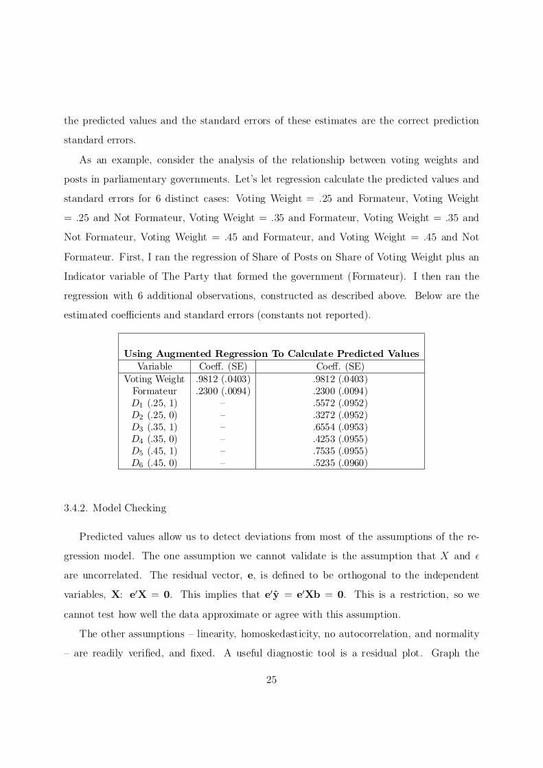
The Wald Criterion.

The general framework for testing in the multivariate context is a Wald Test. Construct

a vector of estimated parameters and a vector of hypothesized parameters. Generically, we

will write these as T and µ0, because they may be functions of regression coe±cients, not

just the coe±cients themselves. De¯ne the vector of deviations of the observed data from

the hypothesized data as d = bfT ¡ µ0. This is a vector of length J .

What is the distribution of d? Under the null hypothesis, E [d] = 0 and V [d] = V[T] =

§. The Wald statistic is:

W = d0§¡1d:

Assuming d is normally distributed, the Wald Statistic follows the Â2 distribution with J

degrees of freedom.

Usually, we do not know §, and must estimate it. Substituting the estimated value of

§ and making an appropriate adjustment for the degrees of freedom, we arrive at a new

statistic that follows the F distribution. The degrees of freedom are J and n ¡ K, which are

the number of restrictions in d and the number of free pieces of information available after

estimation of the model.

In the regression framework, we may implement a test of a set of linear restrictions on

the parameters as follows. Suppose the hypotheses take the form that linear combinations

of various parameters must equal speci¯c constants. For example,

¯ 1 = 0

¯ 2 = 3

and

¯ 4 + 3 = 1

. We can specify the hypothesis as

R¯ = q

31

Where R is a matrix of numbers that correspond to the parameters in the set of linear

equations found in the hypothesis; ¯ is the vector of coe±cients in the full model (length

K), and q is an appropriate set of numbers. In the example, suppose there are 5 coe±cints

in the full model: 0 ¯1

1 0 1 0 1 B C 01 0 0 0 0 ¯ 2B C B CB CB CR¯ = @ 0 1 0 0 0 AB 3 C@ 3 A B C @ A 10 0 1 1 0 ¯4

¯5

The deviation of the estimated value from the true value assuming the hypothesis is true

is

d = Rb ¡ R¯ = Rb ¡ q

If the hypothesis is correct: E [d] = E[Rb ¡ q] = 0.

0 0V [d] = E[dd ] = E[(Rb ¡ R¯)(Rb ¡ R¯)0] = E[R(b ¡ ¯)(b ¡ ¯)0R ]

Because R is a matrix of constants:

0 2 0V [d] = RE[(b ¡ ¯)(b ¡ ¯)0]R = R¾² X0X)¡1R

Because we usually have to estimate the variance of ² the Wald statistic is

(Rb ¡ q)0[R(X0X)¡1R0](Rb ¡ q)=J F =

e0e=(n ¡ K)

Another way to write the F-statistic for the Wald test is as the percentage loss of ¯t.

Suppose we estimate two models. In one model, the Restricted Model, we impose the

hypothesis, and on the other model, the Unrestricted Model, we impose no restrictions. The

F-test for the Wald criterion can be written as

0 0eReR ¡ eueu =J F = 0eueu=(n ¡ K)

Denote the residuals from these models as eR and eU. We can write the residuals from the

restricted model in terms of the residuals from the unrestricted model: eR = y ¡ XbR =

32

y ¡ XbU ¡ X(bR ¡ bU) = eU ¡ X(bR ¡ bU). The sum of squares residuals from the re-

0stricted model is eReR = (eU ¡ X(bR ¡ bU))0 (eU ¡ X(bR ¡ bU))

0 0= eUeU ¡ (bR ¡ bU)0X0X(bR ¡ bU) = eUeU ¡ (RbU ¡ q)0(R(X0X)¡1R0)(RbU ¡ q) So,

the di®erence in the sum of squares between the restricted and the unrestricted model equals

the numerator of the Wald test.

There are two other important testing criteria { likelihood ratio statistics and lagrange

multiplier tests. These three are asymptotically the same. The Wald criterion has better

small sample properties, and it is easy to implement for the regression model. We will discuss

likelihood ratio statistics as part of maximum likelihood estimation.

33

3.5.2. Applications

Three important applications of the Wald Test are (1) tests of speci¯c hypotheses, (2)

veri¯cation of choice of a speci¯cation, and (3) tests of bias reduction in causal estimates,

speci¯cally OLS versus IV. All three amount to comparing the bias due to the more parsi-

monious hypothesized model against the e±ciency gain with that model.

i. Hypothesis Tests: Seats and Votes in England, 1922-2002.

The Cube Law provides an excellent example of the sort of calculation made to test a

concrete hypothesis. The Cube Law states that the proportion of seats won varies as the

cube of the proportion of votes won:

µ ¶3S V = :

(1 ¡ S) 1 ¡ V

We may implement this in a regression model as follows. This is a multiplicative model

which we will linearize using logarithms. There are really two free parameters { the constant

term ® and the exponent ¯.

µ ¶S V

log( ) = ® + log (1 ¡ S) 1 ¡ V

For English Parliamentary elections from 1922 to 2002, the graph of the log of the odds

of the Conservatives winning a seat (labelled LCS) versus the log of the odds of the Conser-

vatives winning a vote (labelled LCV) is shown in the graph. The relationship looks fairly

linear.

Results of the least squares regression of LCS on LCV are shown in the table. The slope

is 2.75 and the intercept is -.07. Tests of each coe±cient separately show that there we would

safely accept the hypothesis that ¯ 0 = 0 and 1 = 3, separately. Speci¯cally, the t-test of

whether the slope equals 3 is 2:75¡3 = 1:25, which has a p-value of .25. The t-test of whether :20

the constant equals 0 is ¡:07¡0 = ¡1:4, which has a p-value of .18. :05

34

Regression Example: Cube Law in England, 1922-2002

Y = Log of the Odds Ratio of Conservative Seats X = Log of the Odds Ratio of Conservative Votes Variable Coe®. (SE) t-test

LCV 2.75 (.20) .25/.2 = 1.25(p = .24)

Constant -0.07 (.05) -.07/.05 = -1.4 (p = .18)

N 21 R2 .91MSE .221

F-test for 2.54 H : ¯ 0 = 0; (p=.10)

¯ 1 = 3

However, this is the wrong approach to testing hypotheses about multiple coe±cients.

The hypothesis has implications for both coe±cients at the same time. An appropriate test

measures how much the vector b0 = (2:75; ¡:07) deviates from the hypothesized vector

¯0 = (3; 0).

After estimating the regression, we can extract the variance-covariance matrix for b,

using the command matrixliste(V). If the null hypothesis is true, then E[b] = 0. The

Wald criterion is d0V[d]¡1d. Because the matrix R is the identity matrix in this example,

i.e., each of the hypotheses pertains to a di®erent coe±cient, V (d) equals V (b). So, the

F-statistic for the Wald criterion is: ¶

1 27:6405 38:2184 F = (:246; ¡:070)

µ38:2184 427:3381

¶ µ :246

2 ¡:070 = :5((¡:246)227:6405 + 2(¡:070)(¡:246)38:2184 + (¡:070)2 427:3381) = 2:54

The probability of observing a deviation this large for a random variable distributed F with 2

and 19 degrees of freedom is .10 (i.e., p-value = .10). This suggests that the data do deviate

somewhat from the Cube Law.

We can implement such tests using the test command in STATA. Following a regression,

you can use test variable names = q to test a single restriction | f(b1; b2; :::) = q1 , such

as test LCV = 3. To test multiple restrictions, you must accumulate successive tests using

35

the option accum. In our example, ¯rst type test LCV = 3, then type test cons = 0,

accum. This returns F = 2:54; p ¡ value = :10.

ii. Choice of Speci¯cation: Energy Survey.

By a speci cation, we mean a speci¯c set of independent variables included in a regression

model. Because there is a tradeo® between e±ciency when irrelevant variables are included

and bias when relevant variables are excluded, researchers usually want to ¯nd the smallest

possible model. In doing so, we often jettison variables that appear insigni¯cant according

to the rule of thumb that they have low values of the t-statistic. After running numerous

regressions we may arrive at what we think is a good ¯tting model.

The example of the Cube Law should reveal an important lesson. The t-statistic on a

single variable is only a good guide about that variable. If you've made decisions about

many variables, you might have made a mistake in choosing the appropriate set.

The F-test for the Wald criterion allows us to test whether an entire set of variables in

fact ought to be omitted from a model. The decision to omit a set of variables amounts to

a speci¯c hypothesis { that each of the variables can be assumed to have coe±cients equal

to 0.

Consider the data from the Global Warming Survey discussed earlier in the course. See

handout. There are 5 variables in the full regression model that have relatively low t-

statistics. To improve the estimates of the other coe±cients, we ought to drop these values.

Also, we might want to test whether some of these factors should be dropped as a substantive

matter.

The F-test is implemented by calculating the average loss of ¯t in the sum of squared

residuals. The information in the ANOVA can be used to compute:

(1276:4912 ¡ 1270:5196)=5 F = = :94754514

1:260436

One may also use the commands test and test, accum.

36

Speci¯cation tests such as this one are very common.

iii. OLS versus Instrumental Variables: Using Term Limits To Correct For Strategic Retire-

ment.

We may also use the Wald criterion to test across estimators. One hypothesis of partic-

ular importance is that there are no omitted variables in the regression model. We cannot

generally detect this problem using regression diagnostics, such as graphs, but we may be

able to construct a test.

Let d = bIV ¡ bOLS. The Wald criterion is d0[V[d]¡1d.

V [bIV ¡ bOLS] = V [bIV ] + V [bOLS ] ¡ Cov[bIV ; bOLS] ¡ Cov [bOLS; bIV ]

Hausman shows that Cov [bOLS; bIV ] = V [bIV ], so

V [bIV ¡ bOLS] = V [bIV ] ¡ V [bOLS]:

^Let X be the set of predicted values from regressing X on Z. The F-test for OLS versus

IV is ^ X)¡1 ¡ (X0X)¡1]¡1dd0[(X0 ^

H = 2s

This is distributed F with J and n-K degrees of freedom, where J is the number of variables

we have tried to ¯x with IV.

37

4. Non-Linear Models

4.1. Non-Linearity

We have discussed one important violation of the regression assumption { omitted vari-

ables. And, we have touched on problems of ine±ciency introduced by heteroskedasticity

and autocorrelation. This and the following subsections deal with violations of the regres-

sion assumptions (other than the omitted variables problem). The current section examines

corrections for non-linearity; the next section concerns discrete dependent variables. Follow-

ing that we will deal brie°y with weighting, heteroskedasticity, and autocorrelation. Time

permitting we will do a bit on Sensitivity.

We encounter two sorts of non-linearity in regression analysis. In some problems non-

linearity occurs among the X variables but it can be handled using a linear form of non-linear

functions of the X variables. In other problems non-linearity is inherent in the model: we

cannot \linearize" the relationship between Y and X. The ¯rst sort of problem is sometimes

called \intrinsically linear" and the second sort is \intrinsically non-linear."

Consider, ¯rst, situations where we can convert a non-linear model into a linear form.

In the Seats-Votes example, the basic model involved multiplicative and exponential param-

eters. We converted this into a linear form by taking logarithms. There are a wide range

of non-linearities that can arise; indeed, there are an in¯nite number of transformations of

variables that one might use. Typically we do not know the appropriate function and begin

with a linear relationship between Y and X as the approximation of the correct relationship.

We then stipulate possible non-linear relationships and implement transformations.

Common examples of non-linearities include:

Multiplicative models, where the independent variables enter the equation multiplicatively

rather than linearly (such models are linear in logarithms);

Polynomial regressions, where the independent variables are polynomials of a set of variables

38

(common in production function analysis in economics); and

Interactions, where some independent variables magnify the e®ects of other independent

variables (common in psychological research).

In each of these cases, we can use transformations of the independent variables to construct

a linear speci¯cation with with we can estimate all of the parameters of interest.

Qualitative Independent variables and interaction e®ects are the simplest sort of non-

linearity. They are simple to implement, but sometimes hard to interpret. Let's consider a

simple case. Ansolabehere and Iyengar (1996) conducted a series of laboratory experiments

involving approximately 3,000 subjects over 3 years. The experiments manipulated the

content of political advertisements, nested the manipulated advertisements in the commercial

breaks of videotapes of local newscasts, randomly assigned subjects to watch speci¯c tapes,

and then measured the political opinions and information of the subjects. These experiments

are reported in the book Going Negative.

On page 190, they report the following table.

E®ects of Party and Advertising Exponsure on Vote Preferences: General Election Experiments

Independent (1) (2) Variable Coe®. (SE) Coe®. (SE)

Constant .100 (.029) .102 (.029)

Advertising E®ects Sponsor .077 (.012) .023 (.034)

Sponsor*Same Party { .119 (.054) Sponsor*Opposite Party { .028 (.055)

Control Variables Party ID .182 (.022) .152 (.031) Past Vote .339 (.022) .341 (.022)

Past Turnout .115 (.030) .113 (.029) Gender .115 (.029) .114 (.030)

39

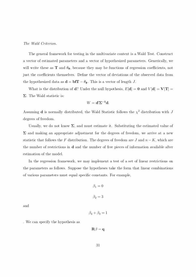
The dependent variable is +1 if the person stated an intention to vote Democratic after

viewing the tape, -1 if the person stated an intention to vote Republican, and 0 otherwise.

The variable Sponsor is the party of the candidate whose ad was shown; it equals +1 if the

ad was a Democratic ad, -1 if the ad was a Republican ad, and 0 if no political ad was shown

(control). Party ID is similarly coded using a trichotomy. Same Party was coded as +1 if

a person was a Democrat and saw a Democratic ad or a Republican and saw a Republican

ad. Opposite Party was coded as +1 if a person was a Democrat and saw a Republican ad

or a Republican and saw a Democratic ad.

In the ¯rst column, the \persuasion" e®ect is estimated as the coe±cient on the variable

Sponsor. The estimate is .077. The interpretation is that exposure to an ad from a candidate

increases support for that candidate by 7.7 percentage points.

The second column estimates interactions of the Sponsor variable with the Party ID vari-

able. What is the interpretation of the set of three variables Sponsor, Sponsor*Same Party

, and Sponsor*Opposite Party. The variables Same Party and Opposite Party encompass

all party identi¯ers. When these variables equal 0, the viewer is a non-partisan. So, the

coe±cient on Sponsor in the second column measures the e®ect of seeing an ad among inde-

pendent viewers. It increases support for the sponsor by only 2.3 percentage points. When

Same Party equals 1, the coe±cient on Sponsor is 11.9. This is not the e®ect of the ad

among people of the same party. It is the di®erence between the Independents and those of

the same party. To calculate the e®ect of the ad on people of the same party we must add

.119 to .023, yielding an e®ect of .142, or a 14.2 percentage point gain.

Interactions such as these allow us to estimate di®erent slopes for di®erent groups, changes

in trends, and other discrete changes in functional forms.

Another class of non-linear speci¯cations takes the form of Polynomials. Many theories

of behavior begin with a conjecture of an inherently non-linear function. For instance, a

¯rm's production function is thought to exhibit decreasing marginal returns on investments,

capital or labor. Also, risk aversion implies a concave utility function.

40

Barefoot empiricism sometimes leads us to non-linearity, too. Examination of data, either

a scatter plot or a residual plot, may reveal a non-linear relationship, between Y and X .

While we do not know what the right functional form is, we can capture the relationship in

the data by including additional variables that are powers of X, such as X1=2 , X 2 , X3 , as

well as X . In other words, to capture the non-linear relationship, y = g(x), we approximate

the unknown function , g(x), using a polynomial of the values of x.

One note of caution. Including powers of independent variables often leads to collinearity

among the righthand side variables. One trick for breaking such collinearity is to deviate

the independent variables from their means before transforming them.

Example: Candidate Convergence in Congressional Elections.

An important debate in the study of congressional elections concerns how well candi-

dates represent their districts. Two conjectures concern the extent to which candidates

re°ect their districts. First, are candidates responsive to districts? Are candidates in more

liberal districts more liberal? Second, does competitiveness lead to closer representation of

district preferences? In highly competitive districts, are the candidates more \converged"?

Huntington posits greater divergence of candidates in competitive areas { a sort of clash of

ideas.

Ansolabehere, Snyder, and Stewart (2001) analyze data from a survey of congressional

candidates on their positions on a range of issues during the 1996 election. There are 292

districts in which both of the competing candidates ¯lled out the survey. The authors con-

structed a measure of candidate ideology from these surveys, and then examine the midpoint

between the two candidates (the cutpoint at which a voter would be indi®erent between the

candidates) and the ideological gap between the candidates (the degree of convergence). To

measure electoral competitiveness the authors used the average share of vote won by the

Democratic candidate in the prior two presidential elections (1988 and 1992).

The Figures show the relationship between Democratic Presidential Vote share and,

respectively, candidate midpoints and the ideological gap between competing candidates.

41

There is clear evidence of a non-linear relationship explaining the gap between the candi-

dates

The table presents a series of regressions in which the Midpoint and the Gap are predicted

using quadratic functions of the Democratic Presidential Vote plus an indicator of Open

Seats, which tend to be highly competitive. We consider, separately, a speci¯cation using

the value of the independent variable and its square and a speci¯cation using the value

of the independent variable deviated from its mean and its square. The last column uses

the absolute value of the deviation of the presidential vote from .5 as an alternative to the

quadratic.

E®ects of District Partisanship on Candidate PositioningN = 292

Dependent Variable Midpoint Gap

Independent (1) (2) (3) (4) (5) Variable Coe®.(SE) Coe®.(SE) Coe®. (SE) Coe®. (SE) Coe®. (SE)

Democratic Presidential -.158 (.369) | -2.657 (.555) | | Vote

Democratic Presidential -.219 (.336) | +2.565 (.506) | | Vote Squared

Dem. Pres. Vote | -.377 (.061) | -.092 (.092) | Mean Deviated

Dem. Pres. Vote | -.219 (.336) | +2.565 (.506) | Mean Dev. Squared

Absolute Value of Dem. Pres. | | | | .764 (.128) Vote, Mean Dev.

Open Seat .007 (.027) .007 (.027) -.024 (.040) -.024 (.040) -.017 (.039) Constant .649 (.098) .515 (.008) 1.127 (.147) .440 (.012) .406 (.015) R2 .156 .156 .089 .089 .110 pMSE .109 .109 .164 .164 .162

F (p-value) 18.0 (.00) 18.0 (.00) 9.59 (.00) 9.59 (.00) 12.46 (.00)

42

Mid

po

int

Be

twe

en

Ca

nd

ida

te I

de

olo

gic

al P

osit

ion

s

0

.2

.4

.6

.8

1

.2 .3 .4 .5 .6 .7 .8 Average Dem. Presidential Vote Share

43

Ide

olo

gic

al

Ga

p B

etw

ee

n C

an

did

ate

s

0

.2

.4

.6

.8

1

.2 .3 .4 .5 .6 .7 .8 Average Dem. Presidential Vote Share

44

Consider, ¯rst, the regressions explaining the midpoint (columns 1 and 2). We expect

that the more liberal the districts are the more to the leftward the candidates will tend. The

ideology measure is oriented such that higher values are more conservative positions. Figure

1 shows a strong relationship consistent with the argument.

Column (1) presents the estimates when we naively include Presidential vote and Pres-

idential vote squared. This is a good example of what collinearity looks like. The F-test

shows that the regression is \signi¯cant" { i.e., not all of the coe±cients are 0. But, neither

the coe±cient on Presidential Vote or Presidential Vote Squared are sign¯cant. Tell-tale

collinearity. A trick for breaking the collinearity in this case is by deviating X from its mean.

Doing so, we ¯nd a signi¯cant e®ect on the linear coe±cient, but the quadratic coe±cient

doesn't change. There is only really one free coe±cient here, and it looks to be linear.

The coe±cients in a polynomial regression measure the partial derivatives of the un-

known function evaluated at the mean of X. Taylor's approximation leads us immediately

to this interpretation of the coe±cients for polynomial models. Recall from Calculus that

Taylor's Theorem allows us to express any function as a sum of derivatives of that function

evaluated at a speci¯c point. We may choose any degree of approximation to the function

by selecting a speci¯c degree of approximation. A ¯rst-order approximation uses the ¯rst

derivatives; a second order approximation uses the second derivatives; and so on. A second

order approximation of an unknown fuction, then, may be expressed as:

1 yi ¼ ® + ¯0 xi + x

2

where " # @f (x)

g0 = @x

0H ;0 ixi

x=x0 " # @2f (x)

H0 = 0

0 +0x0

@x@x x=x0

1 x 2

® = f (x0) ¡ g 0H0 0x0

¯ = g0 ¡ H0x0:

45

The coe±cients on the squares and cross-product terms, then, capture the approximate

second derivative. The coe±cients on the linear values of x equal the gradient, adjusting for

the quadrature around the point at which the data are evaluated (X0 ). If we deviate all of

the variables from their means ¯rst, then the coe±cient on X in the polynomial regression

can be interpreted straightforwardly as the gradient of the (unknown) function at the mean.

Example: Candidate Convergence in Congressional Elections, continued.

Consider the estimates in column (3). We may analyze these coe±cients to ask several @ybasic questions. What is the marginal rate of change? @DP = ¯1 +2¯2DP . Since DP ranges

from .2 to .8, the rate of change in the Gap for a change in electoral competition ranges from

-1.62 when DP = .2 to +1.42 when DP = .8. At what point does the rate of change equal

0 (what is the minimum)? Setting the partial equal to 0 reveals that DP0 = ¡¯ 1 = :517, so 2¯ 2

the candidates are most converged near .5. What is the predicted value of the gap at this

point? 1:127 ¡ 2:657 ¤ :517 + 2:565 ¤ (:517)2 = :438. At the extremes, the predicted values

are .64 (when DP = .8) and .70 (when DP = .2).

If we must choose among several transformations, such as logarithms, inverses, and poly-

nomials, we typically cannot test which is most appropriate using the Wald test. Davidson

and MacKinnon (1981) propose using the predicted values from one of the non-linear anal-

ysis to construct a test. Suppose we have two alternative models: y = X¯ and y = Z°.

Consider a compound model

y = (1 ¡ ¸)bf X¯ + ¸Z° + ²

°. Then, include Z^The J-test is implemented in two steps. First, estimate y = Z° to get Z^ °

^in the regression of y = X¯. The coe±cient on Z° yields an estimate of ¸. Asymptotically, ^ ¸¡0the t-ratio tests which model is appropriate.

SE(¸

Example: Candidate Convergence in Congressional Elections, continued.

An alternative to the quadratic speci¯cation in column (4) is an absolute value speci¯ca-

tion in column (5). Notice that the R2 is slightly better with the absolute value. However,

46

owing to collinearity, it is hard to test which model is more appropriate. I ¯rst regress on

Gap on DP and DP 2 and Open and generated predicted values, call these GapHat. I then

regress Gap on ZG and jDP ¡ :5j and Open. The coe±cient on jDP ¡ :5j is 1.12 with a

standard error of .40, so the t-ratio is above the critical value for statistical signi¯cance.

The coe±cient on ZG equals -.55 with a standard error of .58. The estimated ¸ is not

signi¯cantly di®erent from 0; hence, we favor the absolute value speci¯cation.

47