17 BPF 03 - home.deib.polimi.ithome.deib.polimi.it/rech/Download/17_BPF_03.pdf · SignalRecovery, 2017/2018 –BPF 3 Ivan Rech Band-Pass Filtering 3 2 • Asynchronous Measurement

Signal Recovery, 2017/2018 – BPF 3 Ivan Rech

Sensors, Signals and Noise 1

COURSEOUTLINE

• Introduction

• SignalsandNoise

• Filtering:Band-PassFilters3– BPF3

• Sensorsandassociatedelectronics


Band-Pass Filtering 3 2

• AsynchronousMeasurementofSinusoidalSignals

• PrincipleofSynchronousMeasurements ofSinusoidalSignals

• NoiseFilteringinSynchronousMeasurements

• Lock-inAmplifierPrincipleandWeighting Function

• APPENDIX1:Stage-by-stageviewofSignalsintheLock-inAmplifier

• APPENDIX2:Stage-by-stageviewofNoise intheLock-inAmplifier

• APPENDIX3:Bandwidth,Response TimeandS/NoftheLock-inAmplifier


Asynchronous Measurement of Sinusoidal Signals

3


Asynchronous measurement of sinusoidal signals 4

• Asynchronous (orphase-insensitive) techniquesweredevisedformeasuringasinusoidal signalwithoutneedinganauxiliaryreference thatpointsoutthepeakingtime(i.e.thephaseofthesignal).

• TheyarecurrentlyemployedinACvoltmetersandamperometers.

• Thebasiccircuitsofsuchmetersarethemean-squaredetectorthehalf-waverectifierthefull-waverectifier

• Foracorrectmeasurementoftheamplitudeofthesinusoidal signal,itisnecessarytoavoidfeedingaDCcomponenttotheinputofanasynchronousmetercircuit.Therefore,themetermustbeprecededbyafilterthatcutsoffthelow-frequencies,thatis,aband-passorahigh-passfilter.


Asynchronous measurement of sinusoidal signalswith Mean-Square Detector

5

Low-PassFilter

( ) ( )cosx t A tω ϑ= + ( ) ( ) ( )2 2

2 2cos cos 2 22 2A Ay t A t tω ϑ ω ϑ= + = + +

( )2

2Az t =

t

• Itisapower-meter:theoutputisameasureofthetotal inputmeanpower,sumofsignalpower(proportionaltothesquareofamplitudeA2)plusnoisepower.

• Thelow-passfilterhasNOEFFECTOFNOISEREDUCTION.Infact,itdoesnotaveragetheinput,itaveragesthesquareoftheinput.

• ForimprovingtheS/Nitisnecessarytoinsertafilterbefore theMean-SquareDetector


Low-PassFilter

( ) Az tπ

=

Asynchronous measurement of sinusoidal signals with Rectifier

6

( ) ( )cosx t A tω=

Half-WaveRectifier(HWR)

Full-WaveRectifier(FWR)( ) ( )cosx t A tω=

t

Low-PassFilter

( ) 2Az tπ

=

t

( )4 2

4 2

1cos cos2

T

T

A Az t dt A dT

π

π

ω ϕ ϕπ π

− −

= = =∫ ∫

( )4 2

4 2

2 1 2cos 2 cos2

T

T

A Az t dt A dT

π

π

ω ϕ ϕπ π

− −

= = =∫ ∫

2T πω

=

2T πω

=


Asynchronous measurement of sinusoidal signals with Rectifier

7

• Themeasurementwitharectifier isnotreallyasynchronous,itisself-synchronized.Thesinusoidal signalitselfdecideswhenithastobepassedwithpositivepolarityandwhenpassedwithnegativepolarity(inthefull-waverectifier)ornotpassedatall(inthehalf-waverectifier).

• In such operation, the LPF reduces the contribution of the wide-band noise,thus improving the output S/N. However, this is true only if the input signalis remarkably higher than the noise, i.e. if the input S/N is high.

• Astheinputsignalisreducedthenoisegainsincreasinginfluenceontheswitchingtimeoftherectifier,whichprogressivelylosessynchronismwiththesignalandtendstobesynchronizedwiththezero-crossingsofthenoise.

• ThelossofsynchronizationprogressivelydegradesthenoisereductionbytheLPF.WithmoderateS/NtheimprovementduetoLPFismodest;withlowS/Nitisveryweak.WithS/N< 1 thereisnoimprovement,there isnotevenameasureofthesignal:theoutputisameasureofthenoisemeanabsolutevalue.

• Inconclusion,metersbasedonrectifierscanjustimproveanalreadygoodS/N.Theycan’thelptoimproveamodestS/NanditisoutofthequestiontousethemwhenS/N<1.ForimprovingS/Nitisnecessarytoemployfiltersbeforethemeter.


Synchronous (or Phase-Sensitive) Measurements of Sinusoidal Signals

8


Out+

_

R2R4

R3 RT

VA

Signal and Reference for Synchronization 9

( ) ( )cos mx t A tω ϕ= +

( ) ( )cos mm t B tω=

ACvoltagesupply

REFERENCE

A tobemeasured

Showsthefrequencyandphaseofthesignali.e.pointsoutthepeakinstantsofthesignal

*inthisexample ϕ=0 sincethepreamppassbandlimitismuchhigherthanthesignalfrequencyfm

SIGNALOUT

ϕconstantandknown*

KEYEXAMPLEforthestudyofsynchronousmeasurements andnarrow-bandfiltering

VA

RT =RT(θ)resistancetracksavariableθ,(e.g.a temperatureorastrain);resistancesR2 ,R3 ,R4 areconstant


Out+

_

R2R4

R3 RT

VA

Signal and Reference for Synchronization 10

( ) ( )cos mx t A tω ϕ= +


A tobemeasuredϕconstant

RT e.g.strainsensor,theresistancevariesfollowingamechanicalstrainθ

a)incaseswithconstant strainθconstant A à x(t)isapuresinusoidalsignal

b)incaseswithslowlyvariable strainθ =θ(t)variable A=A(t)à x(t) isamodulatedsinusoidalsignal

SLOWvariations=theFouriercomponentsofA(f)=F[A(t)] havefrequencies f<<fm

VA

KEYEXAMPLEforthestudyofsynchronousmeasurements andnarrow-bandfiltering


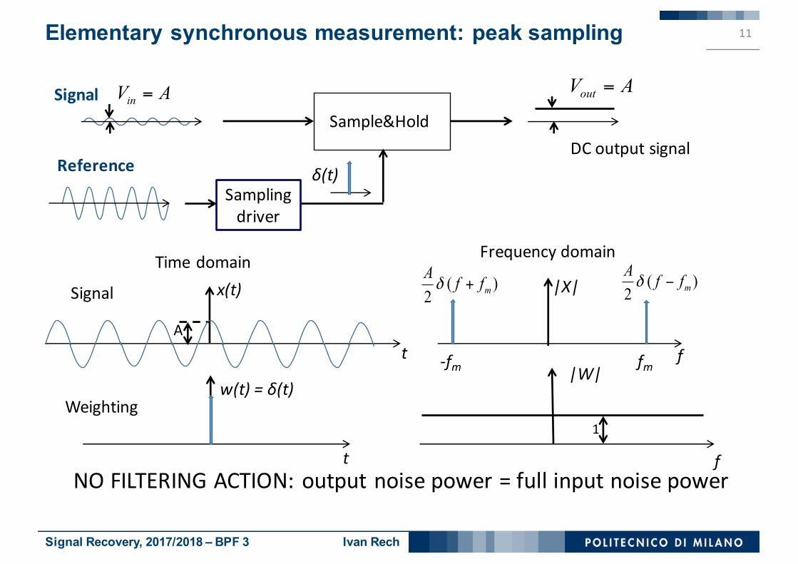
Sample&Hold

outV A=inV A=

DCoutputsignal

Signal

δ(t)

Elementary synchronous measurement: peak sampling 11

fm-fm f

|X|

|W|

f

t

x(t)

t

w(t)=δ(t)

A

( )2 mA f fδ −( )

2 mA f fδ +

Timedomain Frequencydomain

Signal

Weighting

NOFILTERINGACTION:outputnoisepower=fullinputnoisepower

1

Reference

Samplingdriver


Noise Filtering in Synchronous Measurements

12


Synchronous measurement with averaging over many samples N >>1 of the peak

13

t

t

tT-T

rT(t)

t

w(t)

( ) ( ) ( )Tw t m t r t= ⋅

2 1mN f T= ?

( ) ( )cos 2 mx t A f tπ=

T T

m(t)

TotakeNsamplesisequivalenttogate

afree-runningsampler

x(t)


Synchronous measurement with averaging over many samples N >>1 of the peak

14

fm-fm f

|X|

f

|RT|

f

t

t

tT-T

rT(t)

t

fm-fm f

fm-fm

-2fm 2fm

........m(t) |M|

2fm-2fm

FILTERING:narrowbandsatfrequencies0,fm,2fm,3fm ....

........

( ) ( ) ( )Tw t m t r t= ⋅ ( ) * TW f M R≈

12mf T

?


12nf T

Δ =


Poor Noise Filtering by Sample-Averaging 15

fm-fm

|X|

f

|W|2

fm-fm 2fm-2fm

........

3fm-3fm

f

f

Sn1/fnoise whitenoise

• Atfm useful band:itcollects thesignal andsomewhitenoisearoundit• atf=0VERYHARMFULband:itcollects1/fnoiseandnosignal• at2fm ,3fm ,.... harmful bands:theycollect justwhitenoisewithoutanysignal


Synchronous measurement with DC suppression by summing positive peak and subtracting negative peak samples

16

t

x(t)

t

tT-T

rT(t)

t

m(t)

w(t)

T T( ) ( ) ( )Tw t m t r t= ⋅

Totake2Nsamplesisequivalenttogate

afree-runningsampler

NB:equalnumberofpositiveandnegativesamples(zeronetarea)


Synchronous measurement with DC suppression by summing positive peak and subtracting negative peak samples

17

fm-fm f

|X|

f

|RT|

f

t

x(t)

t

tT-T

rT(t)

t

fm-fm f

fm-fm

-2fm 2fm

........m(t) |M|

2fm-2fm

FILTERING:narrowbandsatfm andatodd multiples3fm,5fm ....

........

( ) ( ) ( )Tw t m t r t= ⋅ ( ) * TW f M R≈


Improved Filtering by Sample-Averaging with DC Suppression

18

fm-fm

|X|

ffm-fm 2fm-2fm

........

3fm-3fm

f

f

Sn 1/fnoisewhitenoise

• atfm useful bandthatcollectsthesignal andsomewhitenoisearoundit• Nomorebandatf=0,nomorecollectionof1/fnoise• at3fm ,5fm....residualharmful bandsthatcollect justwhitenoisewithoutanysignal:

howcanwegetridalsoofthem?

|W|2


-T T

Continuous sinusoidal weighting instead of peak sampling 19

fm-fm f

|X|

f

|RT|

f

t

t

tT-T

rT(t)

t

fm-fm f

fm-fm

|M|

TRULYEFFICIENTFILTERING:justonenarrowbandatfm

( ) ( ) ( )Tw t m t r t= ⋅( ) * TW f M R≈


( ) ( )cos mx t A tω=


Optimized noise filtering in synchronous measurement 20

fm-fm

|X|

ffm-fm 2fm-2fm 3fm-3fm

f

f

Sn 1/fnoisewhitenoise

• atfm useful bandthatcollectsthesignal andsomewhitenoisearoundit• Nobandatf=0,nocollection of1/fnoise• Noresidualbandsat3fm ,5fm ...nomorecollectionofwhitenoisewithoutanysignal

Howtoimplementthisoptimizedsynchronousmeasurement?

|W|2


Basic set-up for Synchronous Measurement with optimized noise filtering

21

Sy A∝A DCOutput

InputSignal

Reference

GatedIntegrator

2T

-T T ft fm-fm

( ) ( ) ( )Tw t m t r t= ⋅ ( ) * TW f M R≈Weighting intimedomain Weighting infrequencydomain

z(t)=x(t)·m(t)( ) ( )cos mx t A tω=


AnalogMultiplier

NB:Low-PassFilter(withswitchedparameters)

• NB thereferenceinputtothemultiplier isaSTANDARDwaveform,whichabsolutelydoes NOTdependonthesignal: itisthesameforanysignal!!

• Thereforetheset-up isaLINEAR filter(withtime-variantparameters)

12nf T

Δ =GIcutGIcut


Main Advantages ofSynchronous Measurements with optimized noise filtering

22

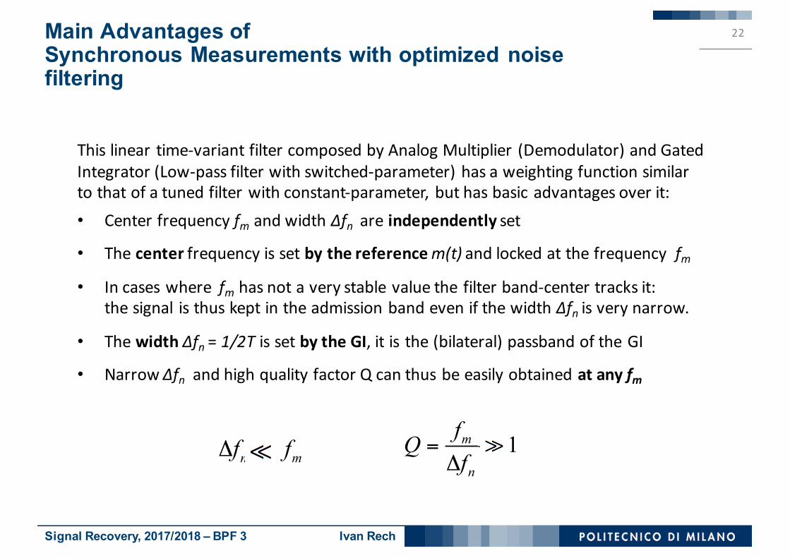
Thislineartime-variantfiltercomposedbyAnalogMultiplier(Demodulator)andGatedIntegrator(Low-passfilterwithswitched-parameter)hasaweightingfunctionsimilartothatofatunedfilterwithconstant-parameter,buthasbasicadvantagesoverit:• Centerfrequencyfm andwidthΔfn areindependentlyset

• Thecenter frequencyissetbythereferencem(t) andlockedatthefrequencyfm

• Incaseswherefm hasnotaverystablevaluethefilterband-centertracksit:thesignal isthuskeptintheadmissionbandevenifthewidthΔfn isverynarrow.

• The width Δfn = 1/2T issetbytheGI,itisthe(bilateral)passbandoftheGI

• NarrowΔfn andhighqualityfactorQcanthusbeeasilyobtainedatanyfm

1m

n

fQf

=Δ

?n mf fΔ =


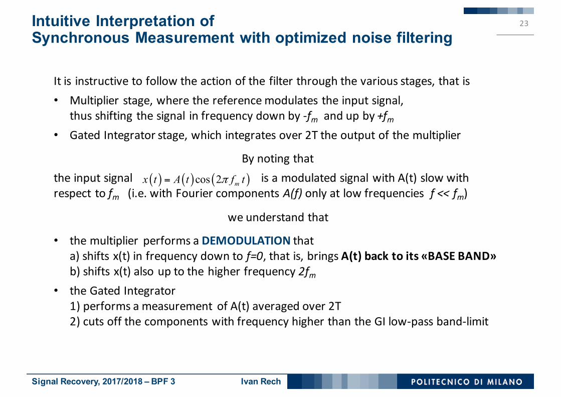
Intuitive Interpretation ofSynchronous Measurement with optimized noise filtering

23

Itis instructivetofollowtheactionofthefilterthroughthevariousstages,thatis• Multiplierstage,wherethereferencemodulatestheinputsignal,

thusshiftingthesignal infrequencydownby-fm andupby+fm• GatedIntegratorstage,whichintegratesover2Ttheoutputofthemultiplier

Bynotingthattheinputsignal isamodulatedsignalwithA(t)slowwithrespecttofm (i.e.withFouriercomponentsA(f) onlyatlowfrequencies f<<fm)

weunderstandthat

• themultiplier performsaDEMODULATION thata)shiftsx(t)infrequencydowntof=0,thatis,bringsA(t)backtoits«BASEBAND»b)shiftsx(t)alsouptothehigherfrequency2fm

• theGatedIntegrator1)performsameasurement ofA(t)averagedover2T2)cutsoffthecomponentswithfrequencyhigherthantheGIlow-passband-limit

( ) ( ) ( )cos 2 mx t A t f tπ=


Lock-in AmplifierPrinciple and Weighting Function

24


From Discrete to Continuous Synchronous Measurements:principle of the Lock-in Amplifier (LIA)

25

Sy A∝

Aquasi-DC

Outputsignal

Inputsignal

Reference



AnalogMultiplier

R

C

wF(α)LPFweightingf.

Theconstant parameterLPFperformsarunningaverageoftheoutputz(t) ofthedemodulator.TheoutputiscontinouslyupdatedandtrackstheslowlyvaryingamplitudeA(t).Thisbasicset-up isdenotedPhase-Sensitive Detector(PSD)andisthecoreofthe instrumentcurrentlycalled Lock-inAmplifier.

FT RC=

Constant-param.Low-PassFilter

Withaveragingperformedbyagatedintegrator,theamplitudeAcanbemeasuredonlyatdiscretetimes (spacedbyatleasttheaveragingtime2T).However,byemployingaconstant-parameterlow-passfilterinsteadoftheGI,continuousmonitoringoftheslowlyvaryingamplitudeA(t)isobtained.


Principle of the Lock-in Amplifier (LIA) 26

Sy A∝A

quasi-DCOutputsignal

Inputsignal

Reference



AnalogMultiplier

R

C

wF(α)LPFweightingf.

Theconstant parameterLPFperformsarunning averageofz(t) overafewTFthatcontinouslyupdatestheoutput

FT RC=

Constant-param.Low-PassFilter

( ) ( ) ( ) ( ) ( ) ( )0 0F Fy t z w d x m w dα α α α α α α∞ ∞

= =∫ ∫

( ) ( ) ( )0 Ly t x w dα α α∞

= ∫

BycomparisonwiththedefinitionoftheLIAweightingfunctionwL(α)

( ) ( ) ( )L Fw m wα α α= ⋅

weseehowthedemodulation andLPFarecombined intheLIA

( ) *L FW f M W≅


Weighting Function wL of the Lock-in Amplifier 27

fm-fm f

|X|

f

f

t

t

t

t

fm-fm f

fm-fm

|M|

( ) ( ) ( )L Fw m wα α α= ⋅( )LW f



2A

2A

2B

2B

( )21

1 2F

F

WfTπ

=+

12 FT

LPFnoisebandwidth(bilateral)

α

α2B

LPFweightingfunctionwF 12n

F

fT

Δ =

( ) *L FW f M W≅


S/N of the Lock-in Amplifier 28

fm-fm

|X|

ffm-fm

f

f

Snb 1/fnoise

whitenoise

|W|2

2A

2A

2

2B⎛ ⎞

⎜ ⎟⎝ ⎠

12n

F

fT

Δ =

SBb

InputSignal(inphase)

Weighting

Noisedensity(bilateral)

22 2 2SA B By A= ⋅ =

2 22 2

2 2yL Bb n Bb nB Bn S f S f⎛ ⎞= ⋅ ⋅Δ = ⋅ ⋅Δ⎜ ⎟

⎝ ⎠

Outputsignal

OutputNoise2 2S

L Bb nyL

yS AN S fn

⎛ ⎞ = =⎜ ⎟Δ⎝ ⎠


Bb Cnb Bb

S fS Sf

= +

BilateralnoisebandwidthoftheLPF


S/N of the Lock-in Amplifier 29

2L Bb n

S AN S f

⎛ ⎞ =⎜ ⎟Δ⎝ ⎠

S/Nequation intermsoftheunilateralparameters

Byintroducing

• fFn theLPFunilateralbandwidth(upperband-limit fornoise),i.e.

• Sbu theunilateralnoisedensity,i.e.

wecanwrite

2L Bu Fn

S AN S f

⎛ ⎞ =⎜ ⎟⎝ ⎠

2n Fnf fΔ =

2 Bb BuS S=

orinpowerterms2 2 2

L Bb n

S AN S f

⎛ ⎞ =⎜ ⎟ Δ⎝ ⎠ n

in phase signal powerhalf power of white noise in the band f

−=

Δ


OutputNoise(𝑆"#$ meandensity intheLPFband)

Case of DC signal with LPF compared to AC signal with LIA 30

Out+

_

R2R4

R3 RT

VA

( )x t A=DCvoltagesupplyVA

RC

FT RC=

LPF

Letusconsidertheset-upofthekeyexample(measurementwithresistivesensor)nowwithDCsupplyvoltageVA equaltotheamplitudeofthepreviousACsupply.ThesignalnowisaDCvoltageequaltotheamplitudeA ofthepreviousACsignal.WithaLPFequaltothatemployedinthepreviousLIAweobtain:

Cy A=∂2

yC nu Fnn S f= ⋅

Outputsignal

∂2

C

C nu FnyC

yS AN S fn

⎛ ⎞ = =⎜ ⎟⎝ ⎠

ThisS/Nmaylookbetterbythefactor 𝟐 thantheS/NobtainedwiththeLIA,butisthisconclusiontrue?NO,suchaconclusionisgrosslywrongbecause𝑺𝒏𝒖$ ≫ 𝑺𝑩𝒖 !!


DC signal and LPF compared to AC signal and LIA 31

fm-fm

ffm-fm

f

f

1/fnoise

whitenoise

|WF|2

2n F nf fΔ =

SBb

DCInputSignal

WeightingoftheLPF


x A=

Bb Cnb Bb

S fS Sf

= +

nbS

1

( ) ( )X f A fδ= ⋅

𝑆"+$ meanspectraldensityintheLPFbandatf=0

𝑆,+ SpectraldensityintheLIAbandatf=fm

Apassbandatf=0 isarisk:1/fnoisegives𝑺𝒏𝒃$ ≫ 𝑺𝑩𝒃 !!


Fake LIA passbands arise from imperfect modulation 32

• Ideally,thereferencewaveformshouldbeaperfectsinusoidatfrequencyfmwithamplitudeB1

• Inreality,deviationsfromtheidealcangeneratespuriousharmonicsatmultiples kfm(k=0,1,2...)withamplitudesBk (smallBk <<B1 incaseofsmalldeviations)

• Moreover,effectsequivalenttoanimperfectreferencewaveformcanbecausedbynon-idealoperation(non-linearity)ofthemultiplier

• Sinceitis

eachspuriousharmoniccomponentofM(f) addstotheLIAweightingfunctionWLaspuriouspassbandatfrequencykfm withamplitudeBk andshapegivenbytheLPF

• Afakepassbandatf=0is particularlydetrimentalevenwithsmallB0 <<B1because itcoversthehighspectraldensityof1/f noise ....

• ....andunluckilyanydeviationfromperfectbalanceofpositiveandnegativeareasofthereferenceproducesaDCcomponentwithassociatedpassbandatf=0 !!

( ) ( ) ( )*L FW f M f W f≅


Theratiocanmatchorexceedtheamplituderatio

sothatthenoise inthefakepassband

canequalorexceedthatinthecorrectpassband

Fake LIA passband at f = 0 33

fm-fm

ffm-fm

f

f

|WL|2

SBb

ImperfectreferencewithDCcomponent

LIAweightingfunction


Bb Cnb Bb

S fS Sf

= +

nbS

( )M f

( )0B fδ⋅ ( )1

2 mB f fδ⋅ −

2 22 1 11 2 2yL Bb n Bu FnB Bn S f S f= ⋅ ⋅Δ = ⋅ ⋅

20B

21

2B⎛ ⎞

⎜ ⎟⎝ ⎠

Cnb Bb Bb

fS S Sf

= +

2n F nf fΔ =

2 21 02B B


APPENDIX

34


Appendix:About the «Gain» of the Lock-in Amplifier 35

Gisdifferentinprinciplefromthegainofanordinaryamplifier: itisaTransfer GainthatcharacterizestheINFORMATIONTRANSFERINFREQUENCYfromfm toDC.

Lock-inAmplifier

Reference

outV GA=inV A=

Output:DCvoltage

Input:ACsignal

2

2in

inVP =

2out outP V=out

Pin

Poutput powerGinput power P

= =

out

in

Voutput voltageGinput voltage V

= =

22

2 2

2

outP

in

VG GV

= =

Vout isaDC voltageVin istheamplitudeofanAC voltageLIAGain however

LIAPowerGain howeverPout isDCpower

Pin isACpower

Therefore anditisprecisely2PG G≠


Appendix1:Stage-by-Stage view of the Signal

in the Lock-in Amplifier

36


Processing Signals with f =fm in the Lock-in Amplifier (LIA) 37

A

quasi-DCOutput

Signal

Reference

z(t)=x(t)·m(t)( ) ( )cos 2 mx t A f tπ ϕ= +

( ) ( )cos 2 mm t B f tπ=

AnalogMultiplier

LPFBandlimit fFn

y(t)

Fn mf f=

• TheMultiplier translatesthesignalintworeplicasshifted infrequencydowntoω=0 anduptoω=2ωm

• TheLPF(thathascutofffFnmuchlowerthanthesignal frequencyfm)passes totheoutputpracticallyonlytheconstantcomponent

Wecangainabetterinsightbyconsideringthespecialcasesofsignalthatwithrespecttothereferenceareinphase [ϕ=0ork·π] andinquadrature [ϕ=π/2or(2k+1)· π/2]

( ) ( ) ( ) ( )cos cos cos cos 22 2m m mAB ABz t A t B t tω ϕ ω ϕ ω ϕ= + = + +

( ) cos2ABy t ϕ≈


Processing Signals with f =fm in the Lock-in Amplifier (LIA) 38



( ) ( )cos sin2m mx t A t A tπ

ω ω⎛ ⎞= + =⎜ ⎟⎝ ⎠

Signalinphaseϕ=0 Signalinquadrature ϕ =π/2

( ) ( ) ( )z t m t x t= ⋅( ) ( ) ( )z t m t x t= ⋅


𝑥 𝑡 𝑥 𝑡

( )2ABy t ≈ ( ) 0y t ≈

2AB

t

t

t

t t

t

t

t

• Anysinusoidcanbeanalyzedassumofin-phaseandinquadraturecomponents

• PhaseselectionbytheLIA:thequadrature components donotcontribute totheoutput( ) ( ) ( ) ( )cos cos cos sin sinm m mx t A t A t A tω ϕ ϕ ω ϕ ω= + = ⋅ − ⋅


Processing Signals with fs ≠ fm in the Lock-in Amplifier (LIA) 39

• Themultiplier convertsthesinusoidalsignaloffrequencyfs ≠fm in:ahigh-frequencycomponentatfh =fs +fmplusalow-frequencycomponentatfl=│fs – fm │

• Thehigh-frequencycomponent iscutoffbytheLPFwithbandlimit fFn<<fm< fs +fm

• Thelow-frequencycomponentisfirstsubjecttoselection infrequencyandisadmittedonlyiffl iswithintheLPFpassband(i.e.if 𝑓1 − 𝑓3 < 𝑓5"),otherwise itis(approximately)cut-off.

• Asignalwithfrequencyfs admittedbythefrequencyselection issubjectedtofurtherselectioninphase: onlyitsin-phasecomponent(ϕ=0)contributestotheoutput.

• Insummary:asinusoidalsignalatfrequencyfs ≠fm- iffs isintheadmissionbandwidthΔfn =2fFn centeredatfm (i.e. 𝑓1 − 𝑓3 < 𝑓5")thesignalisprocessedbytheLIAjustlikeasignalatfs= fm- iffs isoutoftheadmissionbandwidth,itiscutoff


Appendix2:Stage-by-Stage view of Noise

in the Lock-in Amplifier

40


• Selectioninfrequency:noisecomponentsareadmittedonlyfrom(fm – fFn)to (fm +fFn),thatis,withinabandwidthΔfn =2fFn setbytheLPFandcenteredatfm .ThetotalmeanpoweroftheinputnoiseSnu(f) inthisadmissionbandis

• Selectioninphase:onlycomponents inphasewiththereferencecontributetotheoutput.Thenoisecomponentshaverandomphaseϕ ,withuniformprobabilityforallphasesfromϕ=0toϕ=2π.Intheensemblenophaseisfavouredandthemeanpowerisequallysplitbetween in-phaseandquadraturecomponents:onlythein-phase noisemeanpoweristransmittedtotheoutputandishalfofthetotal

Noise in the Lock-in Amplifier (LIA) 41

Lock-inAmplifier

Reference

Noise(unilateraldensity)Snu(f)


( ) ( )2 2nu m Bu m Fnn S f f S f f= Δ = ⋅

( )2

2 212 2o P Bu m Fn

Bn G n S f f= ⋅ ⋅ = ⋅


S/N of the Lock-in Amplifier (LIA) 42

Lock-inAmplifier

Reference

Noise(unilateraldensity)Snu(f)


( ) ( )cos mx t A tω ϕ= +Signal ( )cos2By A ϕ=

Outputsignalpower( )

( )2

22cos 1 cos

2 2 2y P

A BP G Aϕ

ϕ⎡ ⎤⎣ ⎦= = ⋅ ⎡ ⎤⎣ ⎦

( )( )

22 cos2 Bu m Fn

ASN S f f

ϕ⎛ ⎞ =⎜ ⎟⎝ ⎠

( ) ( )2

2

2o P nu m Fn Bu m FnBn G S f f S f f= ⋅ = ⋅Outputnoisepower

( )cos

2 Bu m Fn

S AN S f f

ϕ⎛ ⎞ =⎜ ⎟⎝ ⎠

Signal-to-NoiseRatio: itisconfirmedthat


Notice about the noise transfer in frequency 43

AnalogMultiplier

LPFBandlimit fFn

Reference ( ) ( )cos 2 mm t B f tπ=

StationaryNoise nx(t)withspectrumSxb (bilateral)

nz(t) ny(t)


( )xn t

( ) ( ) ( )z xn t m t n t=

t

t

t

( ) ( )2 2 2 2cosz x mn t n B tω=

Referencewaveform

inputnoisewaveform

multiplieroutnoisewaveform

multiplieroutnoisepowert

We might think that the noise spectrum at the multiplier output is simply thesuperposition of two replicas of the input spectrum shifted up and down by fm ,but this is not exactly the case. The input noise nx(t) is stationary, whereas themultiplier output noise nz(t) is not stationary, it has cyclically varying intensity sothat it is denoted «cyclostationary» noise

However,wewillshowthattheLIAoutputnoisepower canbecomputedwithanequivalentstationary noise,namelywiththeaverageintime ofthecyclostationarynoise



Atthemultiplierout,thenoiseautocorrelationfunctionisnotstationary,butcyclic

Sincetheinputisstationary𝑅77(𝑡, 𝑡 + 𝛾) = 𝑅77(𝛾) ;with𝑚 𝑡 = 𝐵cos 𝜔3𝑡 weget

( ) ( ) ( ) ( ) ( ) ( ) ( ) ( ) ( ) ( ), ,zz xxR t t z t z t m t m t x t x t m t m t R t tγ γ γ γ γ γ+ = + = + ⋅ + = + ⋅ +

TheLPFwith𝑓5" ≪ 𝑓3 performsthenanaverageoveratimemuchlongerthantheperiodoffm.Therefore,thenoisepowerattheoutputoftheLPFcanbecomputedemployingthetime-averageofthecyclostationarynoisenz .Wecanthusemployasequivalent stationaryautocorrelationRzz,eq(ϒ) thetime-averageofRzz(t,t+ϒ)

Inthefrequencydomain,theFouriertransformofRzz,eq(ϒ) canbeemployedasequivalentstationarynoisespectrum

(NB:thespectraldensitieshereareBILATERAL )

( ) ( ) ( )2

, cos cos 22zz m xxBR t t t Rγ γ ω γ γ+ = + + ⋅⎡ ⎤⎣ ⎦

( ) ( ) ( ) ( ) ( ) ( ) ( ), ,zz eq zz xx mm xxR R t t m t m t R K Rγ γ γ γ γ γ= + = + ⋅ = ⋅

( ) ( ) ( ),z eq m xbS f S f S f= ∗



Withsinusoidalreference

wehave

ThankstotheaveragingactionoftheLPF,theoutputpoweractuallycanbecomputedasifthemultiplieroutputwereastationaryspectrum,obtainedbyshiftinginfrequencyby-fmandby+fm theinput spectrumandbysuperposingthetworeplicas.Thisoperationisusuallydenoted«spectrumfolding».Notethatthespectrumfolding doublesthespectraldensityat f=0

sothat

or,withunilateralparameters


( ) ( )2

cos2mm mBK γ ω γ= ( ) ( ) ( )

2

4m m mBS f f f f fδ δ= − + +⎡ ⎤⎣ ⎦

( ) ( ) ( )2

, cos2zz eq m xxBR Rγ ω γ γ= ⋅ ( ) ( ) ( )

2

, 4z eq x m x mBS f S f f S f f= − + +⎡ ⎤⎣ ⎦

( )2

2, 0 2

4o Bz eq BbBn S f S f= Δ = ⋅ Δ

( ) ( ) ( )2 2

, 0 24 4z eq x m x m BbB BS S f S f S= − + + = ⋅⎡ ⎤⎣ ⎦

22

2o Bu FnBn S f= ⋅

Ä

Ä


Appendix3:Bandwidth, Response Time and S/N

of the Lock-in Amplifier

46


ByprocessingasinusoidalsignalofamplitudeA inpresenceofnoiseSBu aLIAgives

• TheequationshowsthatS/NisimprovedbyreducingtheLPFbandlimitfFn .• Thisconclusion,however,isnotindefinitely validinrealcases:thereisalimit

bandwidth,belowwhichtheS/Nisdegraded.• Thereason isthatrealsignalsaremodulatedsinusoids, theyhaveamplitude thatvaries

withtimeA(t) (thoughveryslowlywithrespecttothesignalperiod1/fm )

• Let’sseehowandwhythisreasonlimits theS/Nimprovementobtainedbybandwidthreduction.Thestage-by-stageviewofsignalprocessingreadilyandintuitivelyclarifies it.

Limit to narrow bandwidth convenience 47

( )2 Bu m Fn

S AN S f f

⎛ ⎞ =⎜ ⎟⎝ ⎠

( ) ( ) ( )cos 2 mx t A t f tπ=


Real Signals are Modulated Sinusoids 48

t

t2T

A(t)

( ) ( ) ( )cos mx t A t tω=t2T0

ε

vA

Out+

_

R2R4

R3 RT

VA

RT strainsensorsubjectedtovariablestrainε(t)

( ) ( )cosA A mv t V tω=

strainεà variationΔRT∝ ε à

à Bridgeunbalanceà signalA∝ ε

( ) ( ) ( )cos mx t A t tω=

0

Bridgesupplyvoltage

Bridgeoutputsignal

Amplitudemodulation=BaseBandsignal

TypicalexampleofBaseBandsignal(signaltoberecovered):

Strainε withfiniteduration2T

t


t

Real Signals are Modulated Sinusoids 49

t

ε

Bridgesupply

Strain(Base-Bandsignal)

Bridgeoutputsignal(modulatedsignal)

fm-fm f

f

|ε|

f

fm-fm

|X|

TIMEDOMAIN FREQUENCYDOMAIN

t

x

vA

2T

1. TheBase-bandsignalisnotconstant,itisslowlyvariable,hencethemodulatedsignalhasafinitebandwidthΔfS aroundfm

2. intheLIA,themodulatedsignal isde-modulatedbythemultiplier3. thedemodulatedsignal isthenfilteredbytheLPFintheLIA

ΔfS

ΔfS


Signal de-modulation by the multiplier 50

LIAinput

ffm-fm

fm-fm f

|X|

ffm-fm

t


LIAReference

LIAmultiplieroutput

t

t

|M|

|Z|

x

m

z

-2fm 2fm

t

t

ffm-fm

|ZBB|ffm-fm

|ZUB|

-2fm 2fmzBB

zUBissumof

Upper-bandsignal

Base-bandsignal

plus


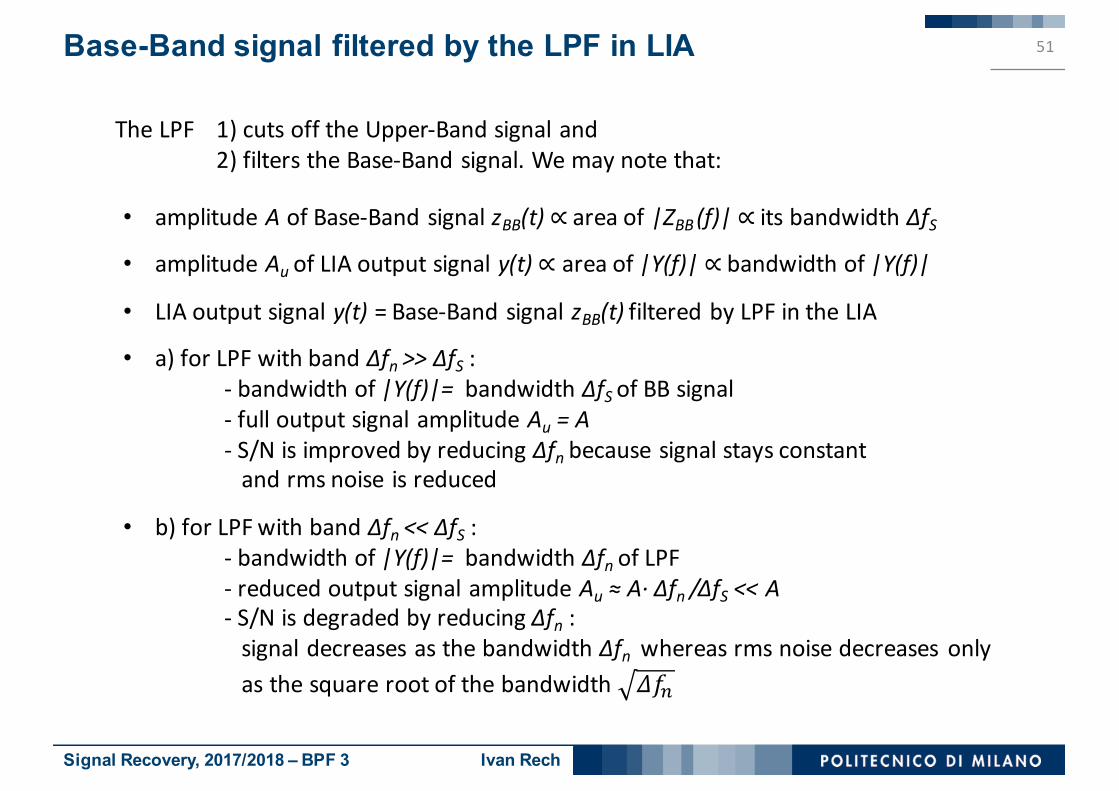
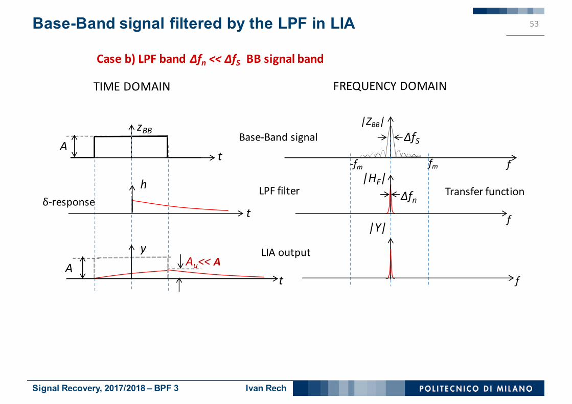
Base-Band signal filtered by the LPF in LIA 51

• amplitudeAofBase-BandsignalzBB(t) ∝ areaof|ZBB(f)| ∝ itsbandwidthΔfS

• amplitudeAu ofLIAoutputsignaly(t) ∝ areaof|Y(f)| ∝ bandwidthof|Y(f)|

• LIAoutputsignaly(t) =Base-BandsignalzBB(t)filteredbyLPFintheLIA

• a)forLPFwithbandΔfn >>ΔfS :- bandwidthof|Y(f)|= bandwidthΔfS ofBBsignal- fulloutputsignalamplitudeAu =A- S/NisimprovedbyreducingΔfn becausesignalstaysconstantandrmsnoise isreduced

• b)forLPFwithbandΔfn <<ΔfS :- bandwidthof|Y(f)|= bandwidthΔfn ofLPF- reducedoutputsignalamplitudeAu ≈A·Δfn /ΔfS <<A- S/NisdegradedbyreducingΔfn :signaldecreasesasthebandwidthΔfn whereasrmsnoisedecreases onlyasthesquarerootofthebandwidth 𝛥𝑓"

TheLPF 1)cutsofftheUpper-Bandsignaland2)filterstheBase-Bandsignal.Wemaynotethat:




tf

|ZBB|zBBBase-Bandsignal

Casea)LPFbandΔfn >>ΔfS BBsignalband

δ-response Transferfunction

A

A LIAoutput

|HF|

y

t

|Y|

hLPFfilter

f

f

-fm fm

Δfn

ΔfS

Au=A




tf

|ZBB|zBB Base-Bandsignal

δ-response

Caseb)LPFbandΔfn <<ΔfS BBsignalband

Transferfunction

A

ALIAoutput

|HF|

t

t

y

LPFfilter

|Y|

Au<<A

f

f

-fm fm

ΔfS

Δfnh


Time-domain study of the LIA response time 54

ThewaveformoftheoutputsignalofaLIAcanalsobecomputeddirectlyintime.With LIAinputsignal 𝑥 𝛼 = 𝑎 𝛼 ⋅ 𝑚 𝛼

LIAreference𝐵 ⋅𝑚 𝛼LPFinLIAweightingfunction𝑤5 𝛼

wehave

Inthesquareofreference𝑚K 𝛼 wecanseparatetheconstantaverageintime 𝑚K

andtheoscillatingcomponent 𝑚K 𝛼 − 𝑚K

andsincetheweighting𝑤5 𝛼 variesveryslowlywithrespecttotheoscillation(inaperioditisalmostconstant)itaveragestheoscillation,sothatwehave

Inotherwords,theoscillatingcomponentiscut-offbytheLPFasillustratedinslide49

( ) ( ) ( ) ( ) ( ) ( ) ( )2F Fy t x Bm w d B a m w dα α α α α α α α

∞ ∞

−∞ −∞= ⋅ = ⋅∫ ∫

( ) ( ) ( ) ( ) ( ) ( )2 2 2F Fy t B m a w d B a m m w dα α α α α α α

∞ ∞

−∞ −∞⎡ ⎤= ⋅ + ⋅ −⎣ ⎦∫ ∫

( ) ( ) ( )2 2 0Fa m m w dα α α α∞

−∞⎡ ⎤⋅ − ≅⎣ ⎦∫


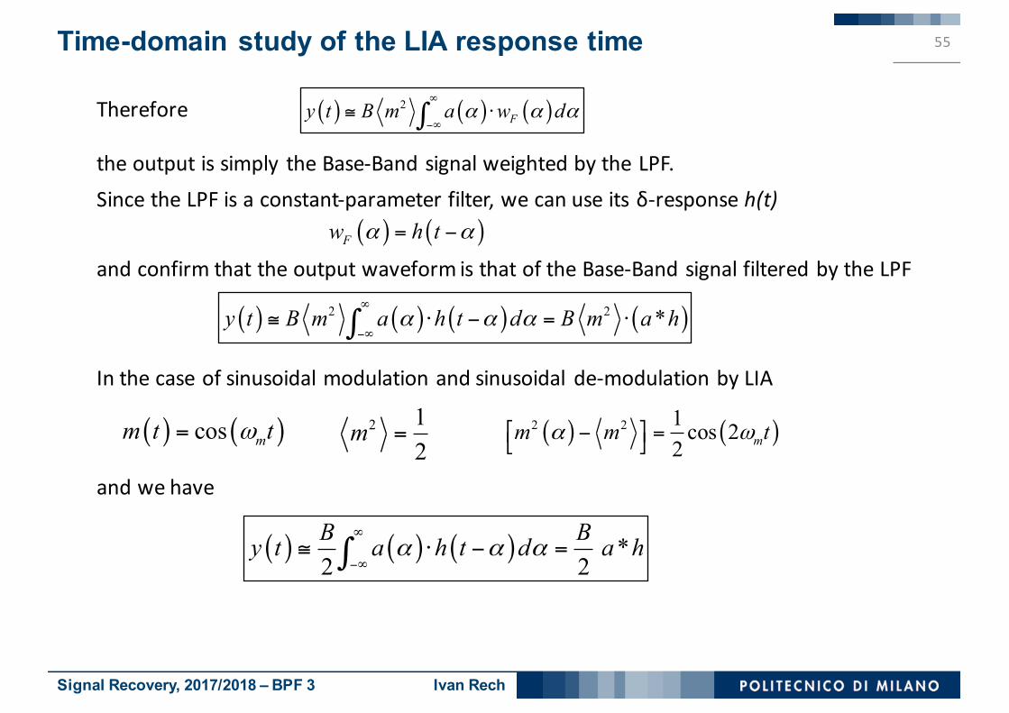
Therefore

theoutputissimplytheBase-BandsignalweightedbytheLPF.SincetheLPFisaconstant-parameterfilter,wecanuseitsδ-responseh(t)

andconfirmthattheoutputwaveformisthatoftheBase-BandsignalfilteredbytheLPF

Inthecaseofsinusoidalmodulationandsinusoidal de-modulationbyLIA

andwehave


( ) ( )cos mm t tω= 2 12

m = ( ) ( )2 2 1 cos 22 mm m tα ω⎡ ⎤− =⎣ ⎦

( ) ( ) ( )2Fy t B m a w dα α α

∞

−∞≅ ⋅∫

( ) ( ) ( ) ( )2 2 *y t B m a h t d B m a hα α α∞

−∞≅ ⋅ − = ⋅∫

( ) ( )Fw h tα α= −

( ) ( ) ( ) *2 2B By t a h t d a hα α α

∞

−∞≅ ⋅ − =∫



t

t

x

y

t

a(t)

t

( ) ( ) ( )1 exp Fh t t t T= ⋅ −

h

Base-Bandsignala(t)=1(t)

Modulatedsignalx(t)(LIAinput)

δ-responseofLPF

LIAoutput

( ) ( ) ( )1 1 exp2 FBy t t t T≅ − −⎡ ⎤⎣ ⎦

Example:stepstrainisappliedtothesensoratt=0andthenmaintainedLPFisasinglepole integratorwithRC=TF

Documents

17 BPF 03 - home.deib.polimi.ithome.deib.polimi.it/rech/Download/17_BPF_03.pdf · SignalRecovery, 2017/2018 –BPF 3 Ivan Rech Band-Pass Filtering 3 2 • Asynchronous Measurement