1666 IEEE TRANSACTIONS ON AUDIO, SPEECH, …articles.ircam.fr/textes/Caetano13a/index.pdf1666 IEEE TRANSACTIONS ON AUDIO, SPEECH, AND LANGUAGE PROCESSING, VOL. 21, NO. 8, AUGUST 2013

1666 IEEE TRANSACTIONS ON AUDIO, SPEECH, AND LANGUAGE PROCESSING, VOL. 21, NO. 8, AUGUST 2013

Musical Instrument Sound Morphing Guided byPerceptually Motivated Features

Marcelo Caetano, Member, IEEE, and Xavier Rodet

Abstract—Sound morphing is a transformation that graduallyblurs the distinction between the source and target sounds. Formusical instrument sounds, the morph must operate across timbredimensions to create the auditory illusion of hybrid musical instru-ments. The ultimate goal of sound morphing is to perform percep-tually linear transitions, which requires an appropriate model torepresent the sounds being morphed and an interpolation functionto obtain intermediate sounds. Typically, morphing techniques di-rectly interpolate the parameters of the sound model without con-sidering the perceptual impact or evaluating the results. Percep-tual evaluations are cumbersome and not always conclusive. Inthis work, we seek parameters of a sound model that favor linearvariation of perceptually motivated temporal and spectral featuresused to guide the morph towards more perceptually linear results.The requirement of linear variation of feature values gives rise toobjective evaluation criteria for sound morphing. We investigateseveral spectral envelope morphing techniques to determine whichspectral representation renders the most linear transformation inthe spectral shape feature domain. We found that interpolation ofline spectral frequencies gives the most linear spectral envelopemorphs. Analogously, we study temporal envelope morphing tech-niques and we concluded that interpolation of cepstral coefficientsresults in the most linear temporal envelope morph.

Index Terms—Musical instrument sounds, sound morphing,source-filter model.

I. INTRODUCTION

S OUND morphing figures prominently among the soundtransformation techniques studied in the literature due to

its great creative potential andmyriad possible outcomes. Soundmorphing has been used in music compositions [1]–[3], soundsynthesizers [4], and even in psychoacoustic experiments, no-tably to study timbre spaces [5]. However, there seems to beno consensus in the literature on which transformations fall intothe category of sound morphing and there certainly is no widelyaccepted definition of the morphing process for sounds. Most

Manuscript received August 21, 2012; revised December 22, 2012; acceptedMarch 26, 2013. Date of publication April 25, 2013; date of current versionMay 08, 2013. This work was supported by the Brazilian government undera CAPES grant (process 4082-05-2) while M. Caetano was pursuing thePh.D. degree at the Analysis/Synthesis team, IRCAM. The associate editorcoordinating the review of this manuscript and approving it for publication wasMr. James Johnston.M. Caetano is with the Signal Processing Laboratory, Foundation for Re-

search and Technology—Hellas, Institute of Computer Science (FORTH-ICS),GR 700133, Heraklion, Crete, Greece (e-mail: [email protected]).X. Rodet is with the Analysis/Synthesis Team, Institut de Recherche at Co-

ordination Acoustique/Musique (IRCAM), 75004, Paris, France.Color versions of one or more of the figures in this paper are available online

at http://ieeexplore.ieee.org.Digital Object Identifier 10.1109/TASL.2013.2260154

Fig. 1. Depiction of image morphing to exemplify the aim of sound morphing.Foundonlineat http://tinypic.com/images/404.gif, currentlypubliclyavailable athttp://paulbakaus.com/wp-content/uploads/2009/10/bush-obama-morphing.jpg.

authors seem to agree that sound morphing involves the hy-bridization of two (or more) sounds by blending auditory fea-tures. One frequent requirement is that the result should fuseinto a single percept, ruling out simply mixing or crossfadingthe sounds [4], [6] because the ear is capable of distinguishingthem due to a number of cues and auditory processes. Still, manydifferent sound transformations are described as morphing, suchas interpolated timbres [4], smooth or seamless transitions be-tween sounds [7] or cyclostationary morphs [8]. In a previouswork [9], we thoroughly reviewed the different types of soundtransformation that are usually termed morphing and evaluatedhow the temporal nature of the morphing transformation (sta-tionary, dynamic, etc) directly interferes in the requirements ofthe process.When morphing musical instrument sounds, we usually want

to transform across timbre dimensions to create the auditory il-lusion of hybrid musical instruments, gradually blurring the cat-egorical distinction between the source and target sounds. Fig. 1illustrates this effect for images. A challenging aspect of suchtransformations is to control the morph on the algorithmic andperceptual levels with a single coefficient , called morphingor interpolation factor [9]. Ideally, we would like to obtain amorphed sound perceptually halfway between source and targetwhen , and be able to recursively repeat the processfor . Equivalently, linear variation of should leadto a perceptually linear transformation. The concept of percep-tual linearity in sound morphing lies at the core of this work,where we use perceptually motivated features to guide the trans-formation and evaluate linearity in the feature domain. We as-sume that linear variation in the feature domain indicates per-ceptual linearity when the features capture perceptually relevantinformation.Most morphing techniques proposed in the literature directly

apply the interpolation principle without taking perceptual as-pects into consideration [4], [6], [7], [10]–[15]. In this work,parameter refers to coefficients fromwhich we can resynthesizesounds (e.g., spectral peaks), while feature refers to coefficientsused to describe or identify a particular aspect of a sound (e.g.,

1558-7916/$31.00 © 2013 IEEE

CAETANO AND RODET: MUSICAL INSTRUMENT SOUND MORPHING GUIDED BY PERCEPTUALLY MOTIVATED FEATURES 1667

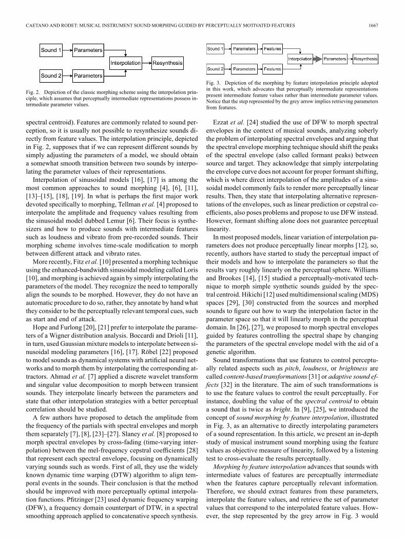
Fig. 2. Depiction of the classic morphing scheme using the interpolation prin-ciple, which assumes that perceptually intermediate representations possess in-termediate parameter values.

spectral centroid). Features are commonly related to sound per-ception, so it is usually not possible to resynthesize sounds di-rectly from feature values. The interpolation principle, depictedin Fig. 2, supposes that if we can represent different sounds bysimply adjusting the parameters of a model, we should obtaina somewhat smooth transition between two sounds by interpo-lating the parameter values of their representations.Interpolation of sinusoidal models [16], [17] is among the

most common approaches to sound morphing [4], [6], [11],[13]–[15], [18], [19]. In what is perhaps the first major workdevoted specifically to morphing, Tellman et al. [4] proposed tointerpolate the amplitude and frequency values resulting fromthe sinusoidal model dubbed Lemur [6]. Their focus is synthe-sizers and how to produce sounds with intermediate featuressuch as loudness and vibrato from pre-recorded sounds. Theirmorphing scheme involves time-scale modification to morphbetween different attack and vibrato rates.More recently, Fitz et al. [10] presented amorphing technique

using the enhanced-bandwidth sinusoidal modeling called Loris[10], andmorphing is achieved again by simply interpolating theparameters of the model. They recognize the need to temporallyalign the sounds to be morphed. However, they do not have anautomatic procedure to do so, rather, they annotate by hand whatthey consider to be the perceptually relevant temporal cues, suchas start and end of attack.Hope and Furlong [20], [21] prefer to interpolate the parame-

ters of a Wigner distribution analysis. Boccardi and Drioli [11],in turn, used Gaussian mixture models to interpolate between si-nusoidal modeling parameters [16], [17]. Röbel [22] proposedto model sounds as dynamical systems with artificial neural net-works and to morph them by interpolating the corresponding at-tractors. Ahmad et al. [7] applied a discrete wavelet transformand singular value decomposition to morph between transientsounds. They interpolate linearly between the parameters andstate that other interpolation strategies with a better perceptualcorrelation should be studied.A few authors have proposed to detach the amplitude from

the frequency of the partials with spectral envelopes and morphthem separately [7], [8], [23]–[27]. Slaney et al. [8] proposed tomorph spectral envelopes by cross-fading (time-varying inter-polation) between the mel-frequency cepstral coefficients [28]that represent each spectral envelope, focusing on dynamicallyvarying sounds such as words. First of all, they use the widelyknown dynamic time warping (DTW) algorithm to align tem-poral events in the sounds. Their conclusion is that the methodshould be improved with more perceptually optimal interpola-tion functions. Pfitzinger [23] used dynamic frequency warping(DFW), a frequency domain counterpart of DTW, in a spectralsmoothing approach applied to concatenative speech synthesis.

Fig. 3. Depiction of the morphing by feature interpolation principle adoptedin this work, which advocates that perceptually intermediate representationspresent intermediate feature values rather than intermediate parameter values.Notice that the step represented by the grey arrow implies retrieving parametersfrom features.

Ezzat et al. [24] studied the use of DFW to morph spectralenvelopes in the context of musical sounds, analyzing soberlythe problem of interpolating spectral envelopes and arguing thatthe spectral envelope morphing technique should shift the peaksof the spectral envelope (also called formant peaks) betweensource and target. They acknowledge that simply interpolatingthe envelope curve does not account for proper formant shifting,which is where direct interpolation of the amplitudes of a sinu-soidal model commonly fails to render more perceptually linearresults. Then, they state that interpolating alternative represen-tations of the envelopes, such as linear prediction or cepstral co-efficients, also poses problems and propose to use DFW instead.However, formant shifting alone does not guarantee perceptuallinearity.In most proposed models, linear variation of interpolation pa-

rameters does not produce perceptually linear morphs [12], so,recently, authors have started to study the perceptual impact oftheir models and how to interpolate the parameters so that theresults vary roughly linearly on the perceptual sphere. Williamsand Brookes [14], [15] studied a perceptually-motivated tech-nique to morph simple synthetic sounds guided by the spec-tral centroid. Hikichi [12] usedmultidimensional scaling (MDS)spaces [29], [30] constructed from the sources and morphedsounds to figure out how to warp the interpolation factor in theparameter space so that it will linearly morph in the perceptualdomain. In [26], [27], we proposed to morph spectral envelopesguided by features controlling the spectral shape by changingthe parameters of the spectral envelope model with the aid of agenetic algorithm.Sound transformations that use features to control perceptu-

ally related aspects such as pitch, loudness, or brightness arecalled content-based transformations [31] or adaptive sound ef-fects [32] in the literature. The aim of such transformations isto use the feature values to control the result perceptually. Forinstance, doubling the value of the spectral centroid to obtaina sound that is twice as bright. In [9], [25], we introduced theconcept of sound morphing by feature interpolation, illustratedin Fig. 3, as an alternative to directly interpolating parametersof a sound representation. In this article, we present an in-depthstudy of musical instrument sound morphing using the featurevalues as objective measure of linearity, followed by a listeningtest to cross-evaluate the results perceptually.Morphing by feature interpolation advances that sounds with

intermediate values of features are perceptually intermediatewhen the features capture perceptually relevant information.Therefore, we should extract features from these parameters,interpolate the feature values, and retrieve the set of parametervalues that correspond to the interpolated feature values. How-ever, the step represented by the grey arrow in Fig. 3 would


require retrieving parameter values from feature values, a no-toriously difficult problem [32]. Instead, in this work, we seekto interpolate parameters of a sound model to obtain morphedsounds whose values of features are as close as possible to theinterpolated feature values. We propose to use the feature valuesas objective measure of the perceptual impact of the morphingtransformation, requiring the features to vary in a straight linewhen changes in equal steps (linearly).Section II introduces the features used in this work along with

their psychoacoustic background from MDS studies. Then, wepresent an overview of the proposed musical instrument mor-phing procedure and the temporal and spectral models used.Next, we discuss morphing the spectral and temporal envelopesguided by the features, followed by the evaluation of linearityin the feature domain. Finally, we conclude and discuss futureperspectives.

II. THE FEATURES USED AS GUIDES

The features used in this work are derived from the acousticcorrelates of timbre spaces from multidimensional scaling(MDS) studies of timbre perception. We include temporaland spectral features to capture the most perceptually salientdimensions of timbre perception, namely, the attack time andthe distribution of spectral energy. The temporal features weuse are the log attack time and the temporal centroid. The spec-tral shape features spectral centroid, spectral spread, spectralskewness, and spectral kurtosis we use are a measure of thebalance of spectral energy.

A. Acoustic Correlates of Timbre Spaces

MDS techniques figure among the most prominent whentrying to quantitatively describe timbre. The MDS algorithmmaps subjective distances (perceptual dissimilarity betweenmusical instrument sounds) into an orthogonal metric spacewhich has the number of dimensions specified by the investi-gator. McAdams [29] and Handel [33] independently proposecomprehensive reviews of the early timbre space studies. Grey[30] investigated the multidimensional nature of the perceptionof musical instrument timbre, constructed a three-dimensionaltimbre space, and proposed acoustic correlates for each di-mension. He concluded that the first dimension correspondedto spectral energy distribution (spectral centroid), the secondand third dimensions were related to the temporal variationof the partials (onset synchronicity and spectral fluctuation).Krumhansl [34] conducted a similar study using synthesizedsounds and also found three dimensions related to attack,synchronicity and brightness. Krimphoff [35] studied acousticcorrelates of timbre spaces and concluded that brightness iscorrelated with the spectral centroid and rapidity of attackwith rise time in a logarithmic scale. McAdams [29] conductedsimilar experiments with synthesized musical instrument tim-bres and concluded that the most salient dimensions were logrise time, spectral centroid and degree of spectral variation.More recently, Caclin [36] studied the perceptual relevance of anumber of acoustic correlates of timbre-space dimensions withMDS techniques and concluded that listeners use attack time,spectral centroid and spectrum fine structure in dissimilarityrating experiments.

In timbre spaces obtained with MDS, the distances betweenpairs of instruments represent the perceptual dissimilarity be-tween them. Timbre space representations are essentially sparsein nature. The space is mostly void and the musical instrumentsoccupy non-overlapping areas. When the morphed sound is per-ceptually intermediate between two musical instrument sounds,it would be placed between them in the underlying timbre space,“filling” the voids and allowing exploration of the sonic con-tinuum. When the features guiding the morph are acoustic cor-relates of timbre dimensions, intermediate feature values wouldcorrespond to intermediate positions in the timbre space.

B. Temporal Features

The attack is the beginning of the acoustic stimulus, presentin all sounds. Psychoacoustic (dis)similarity studies [29], [30],[33]–[37] discovered that the attack is among themost perceptu-ally salient features of musical instrument sounds. These studieshave shown that the attack time is perceived roughly on a loga-rithmic scale.The log attack time is calculated as shown in (1), where

stands for the beginning of the attack and for the end (seeFig. 5). The temporal centroid is the measure of the balance ofenergy distribution along the course of a sound and is calculatedas in (2), where represents the temporal centroid, is time,and is the value of the temporal envelope for time . Thetemporal centroid has been shown [38] to be especially impor-tant when comparing percussive and sustained sounds becausethat is when it varies more significantly, allowing us to distin-guish between the two classes. Still, in the context of strictlysustained sounds, the attack times and temporal centroids varysignificantly enough to be relevant.

(1)

(2)

C. Spectral Shape Features

The spectral shape features are calculated on every frame,which permits to follow their temporal variation. The spectralcentroid is one of the most salient features in psychoacousticstudies [29], [30], [33]–[37] correlated with the verbal attribute“brightness.” Spectral spread is a measure of the bandwidthof the spectrum. Spectral skewness and spectral kurtosis wereshown to be significantly correlated with 2 out of 27 dimensionsof 10 timbre spaces tested in a study [37] of acoustic correlatesof timbre dimensions.The spectral shape features are the first four standardized

moments of the normalized magnitude spectrum viewedas a probability distribution defined in (3), where isthe magnitude spectrum, the frequencies are the possible out-comes, and the probabilities to observe them are .

(3)

Following this definition, the spectral shape features are

(4)


Fig. 4. Depiction of the general steps of the musical instrument sound morphing procedure. There are three distinct parts, temporal processing, spectral processing,and morphing procedure. Blocks with dark grey background represent waveforms, blocks with light grey background represent temporal feature extraction andprocessing, and blocks with white background represent spectral feature extraction and processing.

(5)

(6)

(7)

The spectral centroid is the mean of and the spectralspread is the variance around the mean, shown respectivelyin (4) and (5). The spectral skewness , shown in (6), measuresthe asymmetry of around the spectral centroid, while spec-tral kurtosis, shown in (7), is a measure of the peakedness of

relative to the normal distribution.Notice that the spectral shape features have different units.

The spectral centroid is measured in Hertz, the spectralspread in Hertz squared, and both the spectral skewnessand spectral kurtosis are dimensionless. Furthermore, we canuse different frequency and amplitude scales when calculatingthe spectral shape features to better approximate the spectralinformation that reaches the ear. In this work, we use the melscale [39] to warp the frequency axis and logarithmic amplitudeto better represent loudness perception.

III. MODELING MUSICAL INSTRUMENT SOUNDS

The morphing technique we developed comprises three steps,temporal processing, spectral processing, and the morphingprocedure. Fig. 4 illustrates each step. The blocks representmodeling and processing operations, and the arrows indicatethe order in which they are applied. Blocks with dark graybackground represent waveforms, light gray background repre-sents temporal modeling or processing, and white backgroundis spectral modeling or processing. The temporal processingstep consists of temporal segmentation, temporal alignment,and temporal envelope estimation. The spectral processing stepcomprises sinusoidal plus residual decomposition followedby source-filter modeling of both the sinusoidal and residualcomponents, which are morphed separately and then mixedback together.

A. Temporal Segmentation

Temporal segmentation consists in estimating the boundariesof four perceptually important regions, namely, attack, transi-tion, sustain, and release. Naturally, the sounds can be annotatedby hand [4], [10], but in this work we want to automatically seg-ment the sounds. Ideally, morphing algorithms should take two

Fig. 5. Amplitude/Centroid Trajectory (ACT) model used in the automatictemporal segmentation of musical instrument sounds. The solid line representsthe temporal envelope and the dashed line is the spectral centroid. The numbersstand for the boundaries of the perceptually salient regions, represented by theletters.

(or more) sounds as input and automatically output the morphedsound according to the value of .The automatic segmentation technique we proposed else-

where [40] uses the Amplitude/Centroid Trajectory (ACT)model [41] depicted in Fig. 5, where stands for attack, istransition, is sustain, is release, and is backgroundnoise. The ACT uses the temporal envelope and the spectralcentroid to estimate the boundaries (numbered lambdas) ofthe regions (letters). From these estimations, we calculate thelength of each region.

B. Temporal Alignment

The attack is characterized by fast transients, and the sustainpart is much more stable. Therefore, if we combine a sound thathas a long attack with another sound with a short one withoutprior temporal alignment, the region where attack transients arecombined with more stable partials would not sound natural.To achieve a more perceptually seamless morph, we need totemporally align these regions so that their boundaries coincidebefore combining them.The temporal alignment procedure makes sure that the dif-

ferent regions , , , and are synchronized for the soundsbeing morphed. Algorithmically, temporal alignment meansaligning the numbered lambdas from the ACT model asfollows. For each sound, we measure the length of each region(labeled with letters) by computing the time difference usingthe markers (numbered lambdas). Then, we interpolate be-tween the lengths of the regions according to (8) to obtain theircorresponding lengths in the morphed sound. For the attackwe interpolate from (1) instead. The interpolated lengths arerepresented by a letter that stands for the region and subscriptsindicating both sounds, e.g., for the sustain as shown in (8)

(8)


Fig. 6. Comparison between the spectro-temporal view of the sinusoidal andSF representations. Part a) shows the waveform (top) and spectrogram (bottom).Part b) shows the source (top) and filter (bottom). The source is represented asthe temporal variation of the frequencies of the partials, while the filter is atime-varying spectral envelope. (a) Waveform and spectrogram and (b) sourceand filter

where represents the length of the sustain of the first soundand of the second. The stretch/compress factors andapplied on the first and second sounds respectively are calcu-lated as in (9)

(9)

Finally, we simply time stretch/compress each region by thecorresponding ratio, for instance, by , etc. After temporalalignment, both musical instrument sounds are ready to be mor-phed in the spectral domain.

C. Temporal Envelope Estimation

The amplitudemodulations of musical instrument sounds andspeech are important perceptual cues. Accurate estimation ofthe temporal envelope of a complex waveform (such as musicor speech) is not a trivial task. Ideally, the amplitude envelopeshould outline the waveform connecting the main peaks andavoiding over fitting. In this work, temporal envelope estimationis performed with the true amplitude envelope (TAE) techniquewe developed [42], based on cepstral smoothing. TAE gives areliable estimation that follows closely sudden variations in am-plitude and avoids ripples in more stable regions with near op-timal order selection depending on the fundamental frequencyof the signal.

D. Sinusoidal Plus Residual Decomposition

The aligned musical instrument sounds are decomposedinto a sinusoidal and a residual parts, which are modeledindependently as source and filter. For musical instrumentsounds, the sinusoidal component contains most of the acousticenergy present in the signal because musical instruments aredesigned to have very steady and clear modes of vibration. Theresidual component, obtained by subtraction of the sinusoidalcomponent from the original recording, contains mostly noisymodulations.

E. The Source-Filter Model

The source-filter (SF) model we developed [43] representssource and filter independently, as shown in Fig. 6. The sinu-soidal component comprises a time-varying spectral envelope(filter) and the time-varying frequency values for the partials

Fig. 7. Spectral view of the source-filter model. Each subfigure shows the tra-ditional sinusoidal representation at the top and the source-filter representationat the bottom for one analysis frame.

(source). The residual component is modeled as white noise(source) driving a time-varying spectral envelope (filter).The selection of the spectral envelope estimation method for

the sinusoidal and residual components is very important. Theestimation of the spectral envelope is intimately linked to the SFmodel because it corresponds to the identification of the param-eters of the filter. The main goal of this deconvolution betweensource and filter by means of spectral envelope estimation is toeliminate the harmonic structure of the spectrum, which is as-sociated with the source. Ideally, for the sinusoidal component,the spectral envelope should be a smooth curve that approxi-mately matches the peaks of the spectrum. Wen and Sandler[44] propose to use the channel vocoder to model the filter part.However, Röbel [45] showed that “true envelope” (TE) outper-formed the spectral envelope estimation methods tested, mini-mizing the estimation error for the peaks of the spectrum. Thuswe use TE to estimate the spectral envelope curve of the sinu-soidal component.Fig. 7 presents a comparison of the sinusoidal and the SF rep-

resentation of the amplitudes of partials. The top part of eachsubfigure shows the original spectrum (solid line) and the par-tials (vertical spikes), i.e., the spectral peaks selected by thepeak-picking algorithm. At the bottom part, we see the partialsfrom sinusoidal analysis (vertical spikes) and the spectral enve-lope curve estimated with “true envelope” (solid curve) repre-senting the amplitude of the partials. Both representations re-tain essentially the same information (amplitude and frequencyof partials) in different ways. The frequencies of the partialsare now the values at which we “sample” the spectral envelopecurve. The sinusoidal model has a more accurate representationof the amplitudes of the partials, while the SF representationis much more flexible to perform sound transformations [43].We use linear prediction to estimate the spectral envelope of theresidual component because the envelope curve follows the av-erage energy of the magnitude spectrum rather than fit the am-plitudes of the spectral peaks.

IV. MORPHING MUSICAL INSTRUMENT SOUNDS

The morphing steps comprise spectral envelope morphing,interpolation of frequencies of partials, and temporal envelopemorphing. Each frame is morphed separately in the spectral do-main. The morphed temporal envelope modulates the morphedspectral frames upon resynthesis. For each frame, the morphedspectral envelope gives the amplitude of each partial at the valueof the interpolated frequencies. Sound examples can be found


on http://recherche.ircam.fr/anasyn/caetano/overview.html.This section explains thoroughly each morphing step, payingparticular attention to how the selected features guide spectraland temporal envelope morphs. Linearity in the feature domainwill be used in Section V as objective measure to select arepresentation for the spectral and temporal envelope morphingtechniques. Finally, a listening test was performed to validatethe results of the objective evaluation. Section V presents asystematic evaluation using twenty-six (26) pairs of sounds.

A. Spectral Envelope Morphing

The peaks of the spectral envelope are the frequency regionswhere spectral energy is concentrated. For musical instruments,these perceptually important spectral regions are associatedwith timbre perception [33]. The spectral envelope morphingtechnique must shift in frequency the peaks of the spectralenvelope [24]. Moreover, the amplitudes of these peaks mustalso change accordingly to ensure that the transition will beperceived as smoothly as possible. In other words, the bal-ance of spectral energy should gradually shift from source totarget when the spectral envelope morph is perceived linearly[25]. Therefore, in this work, the spectral envelope morphingtechnique must satisfy both requirements, namely, spectralenvelope peak shifting, and variation of spectral shape featuresas close as possible to a straight line when its parameters areinterpolated in equal steps (i.e., linearly).Fig. 8 shows an example to illustrate the morph using several

representations proposed in the literature: the envelope curve(ENV) [4], [6], cepstral coefficients (CC) [8], dynamic fre-quency warping (DFW) [23], [24], linear prediction coefficients(LPC) [46], reflection coefficients (RC) [46], and line spectralfrequencies (LSF) [47]–[50]. Fig. 8(a) shows the source andtarget envelopes in solid lines and nine intermediate envelopesin dashed and dotted lines corresponding to linearly varyingthe interpolation factor by 0.1 steps. Fig. 8(b) shows the as-sociated values of the spectral shape descriptors for each step.We want the technique that properly accounts for peak shiftingand exhibits linearity in the spectral shape feature domain.Fig. 8 suggests that ENV does not account for peak shifting.

In this case, visually, most spectral shape descriptors changefairly close to a straight line. Interestingly, Fig. 8 reveals thatthe interpolation of CC does not shift the peaks of the spectralenvelope in frequency. In fact, the figure suggests that the resultof interpolating CC is very similar to ENV. The variation ofspectral shape features reveals that these are different transfor-mations. Fig. 8 shows that DFW results in peak shifting. How-ever, the spectral shape features do not vary close to a straightline. Moorer [46] states that LPC do not interpolate well becausethey are derived from impulse responses, and therefore too sen-sitive to changes. Fig. 8 seems to confirm that. In the literature[46], RC are a more robust alternative representation of LPC.Fig. 8 reveals that the transformation is smooth. However, thespectral shape features do not change linearly under interpola-tion of RC. Itakura [51] proposed LSFs as an attractive alterna-tive representation for LPC because of several properties [50],including peak shifting [47]–[49]. The example in Fig. 8 shows

Fig. 8. Spectral envelope morphing guided by spectral shape features. Thefigure shows the variation of the values of spectral shape features when mor-phing spectral envelopes using the main approaches proposed in the literature.Part a) shows the spectral envelope curves and part b) shows the correspondingvariation of feature values. We want the spectral envelope morphing algorithmthat leads to linear variation of spectral shape features. (a) Spectral envelopes.(b) Spectral shape features.

that LSF are indeed suitable parameters to represent and inter-polate the spectral envelopes because the peaks shift properlyand the spectral shape features change rather linearly.


B. Interpolation of Partials Frequencies

The frequencies of the partials, the source in the SF model,carry perceptually important information in the form of tem-poral frequency modulations. For example, when one of thesounds to be morphed presents vibrato, the transformationshould gradually change between more stable partials andvibrato modulations. This can be achieved by interpolating theinterval in cents between frequency and frequency asexpressed in (10), where represents the frequency value ofthe th partial of the first sound, and the frequency value ofthe th partial of the second sound. Equation (11) presents howto interpolate the interval in cents rather than the frequencyvalues and directly. We define the frequency withthe aid of (10) as a fraction of the interval in cents and usethe value of as the frequency of the th interpolated partial.

(10)

(11)

The correspondence between the partials should be carefullyconsidered. Osaka [19] proposed an algorithm to find the op-timal solution to the problem of correspondence between twosets of partials derived from sinusoidal analysis by minimizingthe distance between the frequency intervals for all possiblematches of partials (one-by-one). For near harmonic musicalinstrument sounds, simply matching the partial number mightbe enough. However, one sound might have more partials thanthe other, in which case we could simply discard the unmatchedpartials. Another possibility is to include a harmonic estimate ofthe unmatched partial based on the fundamental frequencyand the harmonic number as . However, this substi-tution can only be used when both sounds are nearly harmonic.When there is a slight harmonic deviation (such as piano sounds,whose upper partials deviate farther and farther from perfectlyharmonic), we must only interpolate the intervals in cents be-tween pairs of partials that were detected. Alternatively, we canuse a model of the inharmonicity to predict the frequencies ofupper partials that were not detected and therefore do not have amatch. In this work, we empirically verified that discarding un-matched partials gives better results for the musical instrumentsounds used than including the harmonic estimation.

C. Temporal Envelope Morphing

In this work, morphing the temporal envelope guided by thetemporal centroid is analogous to morphing the spectral enve-lope because the same estimation and representation techniquescan be applied [25], leading to similar morphing transforma-tions. Also, the temporal centroid is the time-domain counter-part of the spectral centroid , and as such, its values behave inthe same fashion under the same transformations. Analogouslyto Fig. 8, Fig. 9(a) shows the source and target temporal enve-lope curves as solid lines with nine intermediate temporal en-velope curves corresponding to linearly varying by 0.1 steps.Fig. 9(b) shows the corresponding variation of the temporal cen-troid. The temporal envelope morphing techniques consideredare interpolation of the envelope curve (ENV) directly and in-terpolation of the cepstral coefficients (CC) used to represent

Fig. 9. Temporal envelope morphing guided by perceptually motivated fea-tures. The figure shows the temporal envelope curves on the left-hand side andthe corresponding variation of the temporal centroid on the right-hand side.(a) Temporal envelope. (b) Temporal centroid.

it [25]. We discard morphing techniques that shift peaks of theenvelope because this behavior is undesirable for the temporalenvelope.

V. EVALUATION

In total, eighteen (18) musical instrument sounds from theVienna Symphonic Lybrary covering the woodwind, brass, and(plucked and bowed) string musical instrument families wereused in the evaluation. All the sounds used have the same pitch(C4), duration (2s), and dynamics (forte) and present differentattacks (slow, normal, and staccato). The bowed strings alsohave vibrato. The results presented below include a total oftwenty six (26) pairs of sounds from different musical instru-ments. We chose not to morph between the same musical instru-ment with different attacks under the hybrid musical instrumentconstraint.The requirement of linearity in the feature domain can be for-

mulated as a minimum squared error and applied both in thespectral and temporal feature domains. Therefore, the variationof spectral shape features and the temporal centroid are evalu-ated. The interpolation of the frequency of the partials, on theother hand, cannot be formulated or evaluated similarly. Therepresentation that renders the minimum quadratic error is themost linear in the feature domain under consideration, and se-lected as the most appropriate for the morphing scheme.

A. Objective Evaluation

The requirement of linearity of features led to a simple objec-tive error measure to investigate which spectral envelope rep-resentation renders the smallest error when interpolated for allpairs of sounds morphed. Fig. 10 illustrates the error calcula-tion as the deviations between the calculated feature values“o” and the interpolated feature values “x” for each normalizedspectral shape feature . The interpolated feature values“x” are obtained with a straight line connecting the calculatedfeature values for the source and target .The features are all normalized between 0 and 1, so in practice


Fig. 10. Error calculation. The figure depicts the calculation of the feature in-terpolation error. The interpolated feature values obtained as a linear re-gression are represented as “x”, while the calculated feature values arerepresented as “o”.

holds for the interpolated features and the calculatedfeatures are represented as .The error function in (12) is the square root of the sum

of the quadratic deviations between the calculated featurevalues and the interpolated feature values for eachnormalized spectral shape feature , where is the number oflinear steps between and and the subscriptrepresents each spectral shape feature.

(12)

For each pair of sounds, the error is evaluated for eachfeature for all spectral envelope representations considered,and then averaged across features to obtain an error estimation

for each spectral envelope morphing method for a givenpair of sounds. Finally, a global error value for each methodis obtained as the average across all pairs of sounds.

B. Linearity of Spectral Envelope Morphing

Fig. 11 shows the error between the interpolated values ( )and the calculated values ( ) of the spectral shape featuresfor each spectral envelope representation. Part a) shows the errorfor each feature individually for one pair of sounds, and partb) shows the average error across all twenty-six (26) pairs ofsounds used. Part a) shows for each feature, and onthe right-hand side (marked “Total”), representing the averageperformance of each method for each pair of sounds. Noticethat, in practice, is averaged over frames, so Fig. 11also shows the 95% confidence interval across frames.Part b) shows the total error for all twenty-six (26) pairs

of sounds tested. The lowest error bar in this plot gives themost linear spectral envelope morphing method in the spectralshape feature domain for the musical instrument sounds tested.Fig. 11 reveals that interpolation of LSFs presented the smallestquadratic deviation when morphing the spectral envelope.

C. Linearity of Temporal Envelope Morphing

The evaluation of the linearity of temporal envelope mor-phing representations uses the error function analogously

Fig. 11. Error analysis for spectral envelope morphing. The figure shows theerror between the interpolated values ( ) and the calculated values ( )for the spectral shape features. Part a) shows the error for each feature indi-vidually for one pair of sounds, and part b) shows the average error across alltwenty-six (26) pairs of sounds used and the lowest error bar in this plot givesthe most linear spectral envelope morphing method in the spectral shape featuredomain. (a) Single error. (b) Total error.

Fig. 12. Error analysis for temporal envelope morphing. The figure shows theerror between the interpolated values ( ) and the calculated values ( )for the temporal centroid for both temporal envelope morphing methods.

to the spectral counterpart. The feature used is the temporalcentroid , and the temporal envelope morphing methods com-pared are interpolation of curves (ENV) and cepstral coefficients(CC) for the same twenty-six (26) pairs of musical instruments.Fig. 12 shows the comparison of the error values, indicatingthat the interpolation of the cepstral coefficient representation(CC) of the temporal envelope leads to the smallest error. In-terestingly, simple visual inspection of Fig. 9(a) is not enoughto choose between ENV or CC, showing the need to adopt thesmallest quadratic deviation criterion.

D. Perceptual Comparison of Linearity in Sound Morphing

Finally, we performed a listening test to compare the linearityof morphing transformations using musical instrument soundsbetween the SF model developed and traditional sinusoidalanalysis. The SF model used LSFs to morph the spectralenvelopes, while the sinusoidal morphing used the standardinterpolation of frequency and amplitude values. The temporalalignment step is the same for both methods, only the spectralmorphing procedure changes. The listening test presented 11pairs of cyclostationary morphs (with 9 intermediate versionseach) and asked the participants which was “smoother.” Thetest is available online (http://recherche.ircam.fr/anasyn/cae-tano/survey/smoothness.html). Participants could either choosea method, or have no preference. In total, the results of 58participants aged between 22 and 53 were used.The listening test revealed that, in general, linearity depends

on the pair of sounds used. There is no clearly predominant mor-phing technique. For some pairs, many participants manifested


no preference. The task was considered very difficult because itrequired participants to compare the intervals between the ninesteps of the morph, judging several characteristics of sounds atthe same time and remembering them for comparison acrosssteps. The big cognitive load of the task compromised the eval-uations in some cases. The number of steps used was consideredinappropriate because the task relies on memory to perform thecomparison.

VI. CONCLUSION AND FUTURE PERSPECTIVES

In this work, we describe techniques to automatically morphmusical instrument sounds across timbre dimensions guided byperceptually motivated spectral and temporal features that cap-ture the most salient dimensions of timbre perception. The tem-poral features are log attack time and temporal centroid, and thespectral shape features (a measure of the balance of spectral en-ergy) are spectral centroid, spectral spread, spectral skewness,and spectral kurtosis. The concept of morphing by feature inter-polation adopted in this work considers that sounds with inter-mediate values of features are perceptually intermediate whenthe features capture perceptually relevant information. There-fore, the values of the features are considered an objective mea-sure of the perceptual impact of the morphing transformationand the objective evaluation we adopted requires that the fea-tures vary in a straight line when the morphing factor used tocontrol the transformation changes linearly.We describe the temporal and spectral steps of our morphing

algorithm, along with the models used, which include temporalsegmentation and alignment of perceptually salient regions,temporal envelope estimation, and source-filter modeling. Weinvestigate several spectral envelope morphing techniquespreviously proposed in the literature, namely the envelopecurve (ENV), cepstral coefficients (CC), dynamic frequencywarping (DFW), linear prediction coefficients (LPC), reflec-tion coefficients (RC), and line spectral frequencies (LSF), todetermine which representation renders the most linear trans-formation in the spectral shape feature space. We adopted aminimum quadratic deviation approach to evaluate the linearityof the transformations in the feature domain. We found thatinterpolation of line spectral frequencies (LSF) gives the mostlinear spectral envelope morphs and properly shifts the peaksof the spectral envelope in frequency. We also investigatedtemporal envelope morphing techniques guided by featurevalues analogously to the spectral envelope. For the temporalenvelope, we found that cepstral coefficients (CC) give themost linear transformation without shifting the peaks of thetemporal envelope, which is considered undesirable behavior.The innovative aspect of the work described here lies in the

adoption of an objective evaluation criterion (linearity in thefeature domain), which resulted in an error measure that allowscomparison across different morphing techniques. Future per-spectives of this work include investigating the perceptual lin-earity of the results. This challenging task requires human evalu-ation in listening tests. However, the investigator would need todevelop a procedure to efficiently evaluate or compare the per-ceptual linearity of morphing techniques. Nonlinearities play animportant role in musical instruments and their sound produc-tion mechanism, such as attack transients or a brighter sound

when played louder. Perceptual aspects of nonlinear, nonsta-tionary, and inharmonic characteristics of musical instrumentsounds certainly constitute an interesting direction to follow thework towards more gradual morphing transformations.

REFERENCES

[1] T. Wishart, On Sonic Art, ser. On Sonic Art, S. Emmerson, Ed. NewYork, NY, USA: Imagineering Press, 1996.

[2] M. McNabb, “Dreamsong: The composition,” Comput. Music J., vol.5, no. 4, pp. 36–53, 1981.

[3] J. Harvey, “Mortuos plango, vivos voco: A realization at ircam,”Comput. Music J., vol. 5, no. 4, pp. 22–24, 1981.

[4] E. Tellman, L. Haken, and B. Holloway, “Morphing between timbreswith different numbers of features,” J. Audio Eng. Soc., vol. 43, no. 9,pp. 678–689, 1995.

[5] J. M. Grey and J. A. Moorer, “Perceptual evaluations of synthesizedmusical instrument tones,” J. Acoust. Soc. Amer., vol. 62, no. 2, pp.454–462, 1977.

[6] K. Fitz and L. Haken, “Sinusoidal modeling and manipulation usingLemur,” Comput. Music J., vol. 20, no. 4, pp. 44–59, 1996.

[7] M. Ahmad, H. Hacihabiboglu, and A. Kondoz, “Morphing of transientsounds based on shift-invariant discrete wavelet transform and sin-gular value decomposition,” in Proc. Int. Conf. Audio, Speech, SignalProcess., 2009, pp. 297–300.

[8] M. Slaney, M. Covell, and B. Lassiter, “Automatic audio morphing,” inProc. Int. Conf. Audio, Speech, Signal Process., 1996, pp. 1001–1004.

[9] M. Caetano and X. Rodet, “Automatic timbral morphing of musicalinstrument sounds by high-level descriptors,” in Proc. Int. Comput.Music Conf., 2010.

[10] K. Fitz, L. Haken, S. Lefvert, C. Champion, and M. O’Donnel, “Cell-utes and flutter-tongued cats: Sound morphing using Loris and the re-assigned bandwidth-enhanced model,” Comput. Music J., vol. 27, no.3, pp. 44–65, 2003.

[11] F. Boccardi and C. Drioli, “Sound morphing with Gaussian mixturemodels,” in Proc. Int. Conf. Digital Audio Effects, 2001, pp. 44–48.

[12] T. Hikichi, “Sound timbre interpolation based on physical modelling,”Acoust. Science Technol., vol. 22, no. 2, pp. 101–111, 2001.

[13] N. Osaka, “Timbre interpolation of sounds using a sinusoidal model,”in Proc. Int. Comput. Music Conf., 1995.

[14] D. Williams and T. Brookes, “Perceptually motivated audio morphing:Brightness,” in Proc. Audio Eng. Soc., 122nd Conv., 2007.

[15] D. Williams and T. Brookes, “Perceptually motivated audio morphing:Softness,” in Audio Eng. Soc., 126nd Conv., 2009.

[16] R. J. McAulay and T. F. Quatieri, “Speech analysis/synthesis basedon a sinusoidal representation,” IEEE Trans. Acoust., Speech, SignalProcess., vol. ASSP-34, no. 4, pp. 744–754, Aug. 1986.

[17] X. Serra and J. O. Smith, “Spectral modeling synthesis: A sound anal-ysis/synthesis system based on a deterministic plus stochastic decom-position,” Comput. Music J., vol. 14, no. 4, pp. 49–56, 1990.

[18] W. Hatch, “High-level audio morphing strategies,” M.S. thesis, MusicTechnol. Dept., McGill Univ., Montreal, QC, Canada, 2004.

[19] N. Osaka, “Concatenation and stretch/squeeze of musical instrumentalsound using morphing,” in Proc. Int. Comput. Music Conf., 1995.

[20] C. J. Hope and D. J. Furlong, “Endemic problems in timbre morphingprocesses: Causes and cures,” in Proc. Irish Signals Syst. Conf., 1998.

[21] C. J. Hope and D. J. Furlong, “Time-frequency distributions fortimbre morphing: The Wigner distribution versus the STFT,” in Proc.Brazilian Symp. Comput. Music, 1997.

[22] A. Röbel, “Morphing dynamical sound models,” in Proc. IEEE Work-shop Neural Netw. Signal Process., 1998.

[23] H. Pfitzinger, “Dfw-based spectral smoothing for concatenative speechsynthesis,” in Proc. Int. Conf. Spoken Lang. Process., 2004, vol. 2, pp.1397–1400.

[24] T. Ezzat, E. Meyers, J. Glass, and T. Poggio, “Morphing spectral en-velopes using audio flow,” in Proc. Int. Conf. Audio, Speech, SignalProcess., 2005.

[25] M. Caetano and X. Rodet, “Sound morphing by feature interpolation,”in Proc. Int. Conf. Audio, Speech, Signal Process., 2011, pp. 161–164.

[26] M. Caetano and X. Rodet, “Evolutionary spectral envelope morphingby spectral shape descriptors,” inProc. Int. Comput. Music Conf., 2009.

[27] M. Caetano and X. Rodet, “Independent manipulation of high-levelspectral envelope shape features for sound morphing by means of evo-lutionary computation,” in Proc. Int. Conf. Digital Audio Effects, 2010.


[28] S. B. Davis and P. Mermelstein, “Comparison of parametric represen-tations for monosyllabic word recognition in continuously spoken sen-tences,” IEEE Trans. Acoust., Speech, Signal Process., vol. 28, no. 4,pp. 357–366, Aug. 1980.

[29] S. McAdams, S. Winsberg, S. Donnadieu, G. de Soete, and J. Krim-phoff, “Perceptual scaling of synthesized musical timbres: Commondimensions, specifities and latent subject classes,” Psychological Res.,vol. 58, no. 3, pp. 177–192, 2005.

[30] J. M. Grey and J. W. Gordon, “Multidimensional perceptual scaling ofmusical timbre,” J. Acoust. Soc. Amer., vol. 61, no. 5, pp. 1270–1277,1977.

[31] X. Amatriain, J. Bonada, Á. Loscos, J. L. Arcos, and V. Verfaille,“Content-based transformations,” J. New Music Res., vol. 32, no. 1,pp. 95–114, 2003.

[32] V. Verfaille, U. Zölzer, and D. Arfib, “Adaptive Digital Audio Effects(a-DAFx): A new class of sound transformations,” IEEE Trans. Audio,Speech, Lang. Process., vol. 14, no. 5, pp. 1817–1831, Sep. 2006.

[33] S. Handel, “Timbre perception and auditory object identification,” inHearing, B. Moore, Ed. New York, NY, USA: Academic, 1995, pp.425–461.

[34] C. L. Krumhansl, “Why is musical timbre so hard to understand?,”in Structure and perception of electroacoustic sound and music, S.Nielzén and O. Olsson, Eds. New York, NY, USA: Excerpta Medica,1989, pp. 43–54.

[35] J. Krimphoff, S. McAdams, and S. Winsberg, “Charactérisation dutimbre des sons complexes. II: Analyses acoustiques et quantificationpsychophysique,” J. Physique IV, vol. 4, no. 1, pp. C5.625–C5.628,1994.

[36] A. Caclin, S. McAdams, B. K. Smith, and S. Winsberg, “Acoustic cor-relates of timbre space dimensions: A confirmatory study using syn-thetic tones,” J. Acoust. Soc. Amer., vol. 118, no. 1, pp. 471–482, 2005.

[37] S. McAdams, G. Bruno, P. Susini, G. Peeters, and V. Rioux, “A meta-analysis of acoustic correlates of timbre dimensions (a),” J. Acoust.Soc. Amer., vol. 120, no. 5, pp. 3275–3275, 2006.

[38] J. Skowronek and M. McKinney, “Features for audio classification:Percussiveness of sounds,” in The language of electroacoustic music,W. Verhaegh, E. Aarts, and J. Korst, Eds. Dordrecht, The Nether-lands: Springer Netherlands, 2006, pp. 103–118.

[39] S. S. Stevens, J. Volkman, and E. Newman, “A scale for the measure-ment of the psychological magnitude of pitch,” J. Acoust. Soc. Amer.,vol. 8, no. 3, pp. 185–190, 1937.

[40] M. Caetano, J. J. Burred, and X. Rodet, “Automatic segmentation ofthe temporal evolution of isolated acoustic musical instrument soundsusing spectro-temporal cues,” in Proc. Int. Conf. Digital Audio Effects,2010.

[41] J. Hajda, “A new model for segmenting the envelope of musical sig-nals: The relative salience of steady state versus attack, revisited,” inProc. Audio Eng. Soc. Conv. 101, 11, 1996.

[42] M. Caetano and X. Rodet, “Improved estimation of the ampli-tude envelope of time-domain signals using true envelope cepstralsmoothing,” in Proc. Int. Conf. Audio, Speech, Signal Process., 2011,pp. 4424–4427.

[43] M. Caetano and X. Rodet, “A source-filter model for musical instru-ment sound transformation,” in Proc. Int. Conf. Audio, Speech, SignalProcess., 2012, pp. 137–140.

[44] X. Wen and M. Sandler, “Source-filter modeling in the sinusoidal do-main,” J. Audio Eng. Soc., vol. 58, no. 10, pp. 795–808, 2010.

[45] A. Röbel and X. Rodet, “Efficient spectral envelope estimation and itsapplication to pitch shifting and envelope preservation,” in Proc. Int.Conf. Digital Audio Effects, 2005, pp. 30–35.

[46] J. A.Moorer, “The use of linear prediction of speech in computer musicapplications,” J. Audio Eng. Soc., vol. 27, no. 3, pp. 134–140, 1979.

[47] K. Paliwal, “Interpolation properties of linear prediction parametricrepresentations,” in Proc. Eur. Conf. Speech Commun. Technol., 1995,pp. 1029–1032.

[48] R. Morris andM. Clements, “Modification of formants in the line spec-trum domain,” IEEE Signal Process. Lett., vol. 9, no. 1, pp. 19–21, Jan.2002.

[49] I. V. McLoughlin, “Review: Line spectral pairs,” Signal Process., vol.88, no. 3, pp. 448–467, 2008.

[50] T. Backström and C. Magi, “Properties of line spectrum pair polyno-mials—A review,” Signal Process., vol. 86, pp. 3286–3298, 2006.

[51] F. Itakura, “Line spectrum representation of linear prediction coeffi-cients of speech signals,” J. Acoust. Soc. Amer., vol. 57, pp. S35–S35,1975.

Marcelo Caetano received the Ph.D. degree in signal processing from UPMCParis 6 University in 2011 under the supervision of Xavier Rodet. He is presentlya Marie Curie postdoctoral fellow with the Signal Processing Laboratory atFORTH. Dr. Caetano’s research interests range from musical instrument soundsto music modeling, including analysis/synthesis models for sound transforma-tion and music information retrieval.

Xavier Rodet is currently emeritus researcher at IRCAM on the Analysis/Syn-thesis team. He has beenworking on digital signal processing for speech, singingvoice synthesis, and automatic speech recognition. Computer music is his othermain domain of interest. Dr. Rodet has been working on understanding spectro-temporal patterns of musical sounds and on synthesis-by-rules.

Documents

1666 IEEE TRANSACTIONS ON AUDIO, SPEECH, …articles.ircam.fr/textes/Caetano13a/index.pdf1666 IEEE TRANSACTIONS ON AUDIO, SPEECH, AND LANGUAGE PROCESSING, VOL. 21, NO. 8, AUGUST 2013