1

16.513 Control Systems

Lyapunov Stability: An introduction to Nonlinear/Uncertain Systems

1

Stability for a linear systemThe system:

DuCxy Bu,Axx +=+=

Basic req irement for a s stem:Basic requirement for a system:• If a bounded input is applied, a bounded output

should be produced. BIBO stable.• If the input is removed, the output will vanish

gradually y(t) → 0, as t → ∞. output stable• If you remove the input, the state will vanish

2

If you remove the input, the state will vanishx(t) → 0, as t → ∞. Internal stable (asymptotically)

These stability notions are closely related. Internal stability is fundamental. For LTI sys, internalstability implies the others.

2

Internal stability for a linear system

Atxex(t) =It is about the behavior of the zero input response:

The system: DuCxy Bu,Axx +=+=

0xex(t) =

• Re(λi)<0, for all .i, then as t → ∞, eAt→ 0, x(t) always converges to 0. → Asymptotically stable

• Re(λi) > 0, for some .i. Some entries of eAt diverge.There exist x0 such that x(t) grows unbounded. Unstable

(λ ) 0 f ll i ll i l i h 0 l

Based on the solution, we have the following results:

3

• Re(λi) ≤ 0 for all .i, all eigenvalues with 0 real parts are simple, eAt is bounded but not converge to 0. Critical case

• Re(λi) ≤ 0 for all .i, some eigenvalues with 0 real parts are repeated, eAt unbounded; x(t) unbounded for some x0 unstable

The most desirable is asymptotic stability, ensuring robustness

What if we have a nonlinear system: ),( txfx =

For instance, sat(Fx) BAxx += sat(Fx)

• This is a very common case.

u=Fx

Most physical control systems have this form.

Another case: differential inclusion

ΩA:Axx ∈∈ Can be used to describe uncertaintime-varying systems

4

time varying systems

• The explicit solutions for these systems cannot be obtained.

• How can we analyze stability, performance?

3

Example: Consider a switched system

,113/1131A,11

11A ,xA x,Ax 2121 ⎥⎦⎤

⎢⎣⎡

−−−=⎥⎦

⎤⎢⎣⎡

−−−=∈

Both A1 and A2 have eigenvalues at -1+ j and -1 – j. The switching rule is arbitrary, i.e., dx/dt can take either A1x or A2x.switching rule is arbitrary, i.e., dx/dt can take either A1x or A2x.

• Is the system stable?

An earlier conjecture: if αA1+(1-α)A2 is stable for all α∈[0,1], maybe the system should be stable.

For this particular system the eigenvalues of αA +(1 α)A

5

For this particular system, the eigenvalues of αA1+(1-α)A2have real part -1 for all α∈[0,1].

• However, there is a switching rule to make the trajectoriesdiverge.

,113/1131A,11

11A ,xA x,Ax 2121 ⎥⎦⎤

⎢⎣⎡

−−−=⎥⎦

⎤⎢⎣⎡

−−−=∈

Ob i E f

0.8

Observation: Even fortwo stable systems, there may exist a switching rule to makethe system unstable.

Question: How can -0.4

-0.2

0

0.2

0.4

0.6 A1x

A2x

6

Quest o : ow cawe guarantee stability?

-3 -2 -1 0 1 2 3-0.8

-0.6

4

Example: an opposite case. Consider the switched system

,1.03/111.0A,1.03-

11.0A ,xA x,Ax 2121 ⎥⎦⎤

⎢⎣⎡−=⎥⎦

⎤⎢⎣⎡=∈

Both A1 and A2 are unstable. Question: Is there a particular switching rule to make the system stable?

0

0.2

0.4

0.6

0.8

A1x Yes.

7-0.8 -0.6 -0.4 -0.2 0 0.2 0.4 0.6 0.8 1 1.2

-1.2

-1

-0.8

-0.6

-0.4

-0.2

0

A2x

Stability analysis without solving differentialequations

Lyapunov’s approach:

qCan be applied to complicated systemsCan also be used for performance analysis

8

5

The vector field, trajectories: a geometric view

f(x)x =The system

It actually describes a vector field. f(x)x =

For a given x, f(x) is the vectorwhich describes the directionx(t) heads to and how fast it goes (velocity): x(t0+δt) = x(t0)+δt f(x)

Starting from a point x0, a smooth curve

x velocity:xposition :x

9

can be constructed such that the vectorsalong the curve is tangential to it.

x0

This smooth curve is called a trajectoryAlso a solution to f(x)x =

Lyapunov stability: a first glimpsef(x)x =The system

• Usually it is hard/impossible to get the explicit solution• It is possible to characterize some properties of the• It is possible to characterize some properties of the

vector field, e.g., its relation w.r.t some reference set.

• For example, there is a continuum of ellipsoidsSame shape, different radius, from0 to ∞.

• S ll th t f( ) i t

10

• Suppose all the vectors f(x) point inward of every ellipsoid.

• What can we conclude from here?Every trajectory goes to smaller and smaller ellipsoidsEventually converges to 0. ⇒ Stability

6

Generalization

• Observation: We can use more general reference sets than ellipsoids

• As long as all the vectors points inward of each

11

boundary, we can still conclude stability.

Q: How to describe mathematically this property?How to describe the shape of a reference set?

Positive definite function and level sets

Definition: A function V: Rn → R is said to be positive definite if V(x) > 0 for all x ≠ 0;

iti i d fi it if V( ) ≥ 0 f ll positive semi-definite if V(x) ≥ 0 for all x ; negative definite if V(x) < 0 for all x ≠ 0. negative semi-definite if V(x) ≤ 0 for all x .

Given a positive semi-definite V. For a positive number r, denote r3

12

LV(r):= x∈Rn: V(x) ≤ r

LV(r) is said to be a level set of V.

Clearly, LV(r1)⊆ LV(r2) if r1< r2.

r1

r23

7

Quadratic functions and ellipsoids ( §3.9 )

• These are the most popular choices of functions andlevel sets.

• Given a symmetric matrix P=PT (pij=pji). A quadratic function can be defined as

V(x) = xTPxn n

13

ji

n

1i

n

1jij

T xxp PxxV(x) ∑∑= =

==

Theorem: A symmetric matrix P is positive definiteif and only if its eigenvalues are all positive.

Review:

Theorem: A symmetric matrix P is positive definiteiff there exists a nonsingular matrix N such that P=NNT.

14

8

Matrix inequalities:Given two real symmetric matrices P and Q, we say that

P > Q if P −Q> 0 (P−Q positive definite) P ≥ Q if P − Q ≥0 (P−Q positive semi-definite)≥ Q Q ≥ ( Q p )P < Q if P−Q < 0 (P−Q negative definite)P ≤ Q if P − Q ≤0 (P−Q negative semi-definite)

It is easy to see that, • If P < Q, and X is nonsingular, then X’PX < X’QX • If P< Q and X is singular then X’PX ≤ X’QX

15

• If P< Q, and X is singular, then X PX ≤ X QX

Level sets of quadratic functionsConsider P = PT > 0 (symmetric + positive definite).Let V(x)=xTPx. V is positive definite. • What are the level set LV(r)=x∈Rn: xTPx ≤ r?What are the level set LV(r) x∈R : x Px ≤ r?

Example: 22

21

TT 4xxx4001xPxxV(x) +=⎥⎦

⎤⎢⎣⎡==

• The level set LV(1)– The ellipsoid includes (0,0.5)

and (1 0)x2

(0 0 5)

16

and (1,0). x1

(1,0)

(0,0.5)

– The boundary is the set x: xTPx=1

9

Example: ⎥⎦⎤

⎢⎣⎡=⎥⎦

⎤⎢⎣⎡== ββ

ββcossinsin-cos Ux,U40

01UxxPx(x)V TT1

T1

LV1 (1) has the same shapeas LV(1). Rotate by β.x1

x2

For a general P=PT > 0. Let λmax be the maximal eigenvalue, λmin be the smallest eigenvalue.

The level set LV(1) is an ellipsoid with long axis

The one with ⎥⎦⎤

⎢⎣⎡= 40

01P

17

V(1/λmin)1/2 and short axis (1/λmax)1/2

To reflect the dependence of the ellipsoid on the matrixP, we denote ε(P,r):=LV(r), where V(x)=x’Px

rPxx':Rxr)(P, n ≤∈=ε

Family of level setsConsider P = PT > 0 (symmetric + positive definite).Let V(x)=xTPx.

• What is the relation between ε(P 1) and ε(P s2)?• What is the relation between ε(P,1) and ε(P,s )? For a subset X of Rn and a positive number k, denote kX=kx: x∈X → a scaled set.

• Then ε(P,s2) = s ε(P,1). Note that 222

2

sPxx':Rx)sε(P1Px x':Rxε(P,1)≤∈=

≤∈=

18

Small: ε(P,1/4)Middle: ε(P,1)Large: ε(P,4)

sPx x:Rx)sε(P, ≤∈=

10

We turn back to the stability problem for a systemLyapunov Stability:

f(x)x =• How to describe the property that all vector point

inward of an ellipsoid? • Let the ellipsoid be: ε(P,r).

Its boundary is the set x: x’Px = r• Let x0 be a point on the boundary.

The vector perpendicular to thePx0

19

p ptangential surface of the ellipsoidat x0 is Px0

• The vector f(x0) points inward iff 0)f(x,Px 00 < 0)f(xP'x 00 <

x0

f(x0)

In summary, for the systemTheorem: Given P=PT>0. If xTPf(x) < 0 for all x≠0,then the system is asymptotically stable.

f(x)x =

P E planation:Px0

x0

f(x0)

Explanation: • On the boundary of each ellipsoid

ε(P,r), the vector f(x) points strictly inward of the ellipsoid.

• A trajectory starting from each boundary will reach smaller and

20

boundary will reach smaller and and smaller boundaries,

• Eventually, converge to the originSuch a stability is called quadratic stability. The level setsare called contractively invariant ellipsoids.

11

Another interpretation: • Given a quadratic function V(x)=x’Px, P=P’>0.

∂V/∂x=2Px.• Along a trajectory x(t) of the system, V is a function g j y ( ) y ,

of time, V(x(t)).• The time derivative of V is

Pf(x)2xf(x)xVx

xVV ,

,,

=⎟⎠⎞

⎜⎝⎛

∂∂

=⎟⎠⎞

⎜⎝⎛

∂∂

=

h di i ’ f( ) 0 i li h ( ( )) i

21

• The condition x’Pf(x) < 0 implies that V(x(t)) is strictly decreasing.

• Hence V(x(t)) → 0 as t → ∞.• x(t) ∈ ε(P,r) for r → 0. • x(t) → 0.

With a more general positive-definite function V(x).Let the derivative with respect to x be ∂V/∂x.

Theorem: If (∂V/∂x)Tf(x,t) < 0, for all x≠0, all t>0,

Consider the system ),( txfx =

Theorem: If (∂V/∂x) f(x,t) 0, for all x≠0, all t 0, then the system is asymptotically stable.

∂V/∂x: perpendicular to thetangential surface.

Potential: the vector f(x,t) can

22

This is the fundamental theorem of stability for nonlinear, uncertain and time-varying systems.It is called Lyapunov stability theorem. The function Vis called the Lyapunov function.

be allowed to have uncertainty

12

Now we work on the linear system: Axxfx == )(

Applying the condition for quadratic stability, we have

Theorem: If there exists a P=PT>0, such thatATP+PA < 0 (negative definite), (1)

Then the system is asymptotically stable.

Explanation: The original stability condition is

This is called Lyapunov stability theorem for linear systems

23

xTPf(x)=xTPAx<0 for all x≠0 (2)Note that xTPAx=(xTPAx)T=xTATPx. (2) is equivalentto xT(PA+ATP)x < 0 for all x≠0 (3)(3) ⇔ (1). Note that PA+ATP is symmetric.

relates to the earlier condition

How the stability condition, ∃ P=P’>0 s.t. A’P+PA < 0 (1)

Re(λ ) < 0 for all eigenvalues λ s of A (2)Re(λk) < 0 for all eigenvalues λk’s of A (2) Conclusion: They are the same.

Theorem: All eigenvalues of A have negative real parts iff for any N=N’> 0, the Lyapunov equation

A’P + P A= − N (*)

24

AP P A N ( )has a unique solution P=P’ > 0.

13

Theorem: All eigenvalues of A have negative real parts iff for any N=N’> 0, the Lyapunov equation

A’P + P A= − N (*)

Look again at the theorem:

AP P A N ( )has a unique solution P=P’ > 0.

• It concludes more than the existence of P such thatA’P+PA < 0.

• In fact, you can construct a P > 0 such that A’P+PA equals any given negative definite matrix −N

25

equals any given negative definite matrix N.

Example:⎥⎦⎤

⎢⎣⎡

−−−−== 21

0.21AAx,x

Pick N = -I, and solve A’P + PA = − N (use matlab P=lyap(A’ I) we obtain(use matlab P lyap(A ,I), we obtain

P = 0.6296 -0.1296-0.1296 0.2630

-0.5

0

0.5

1

1.5

2

2.5

Boundary of (P 1) th t f h

26

-1.5 -1 -0.5 0 0.5 1 1.5-2.5

-2

-1.5

-1ε(P,1), the set of x such that x’Px=1.

Each line segment starts at a point x on the boundary and Ends at x+Ax*k for some scaling k. It shows the direction of Ax

14

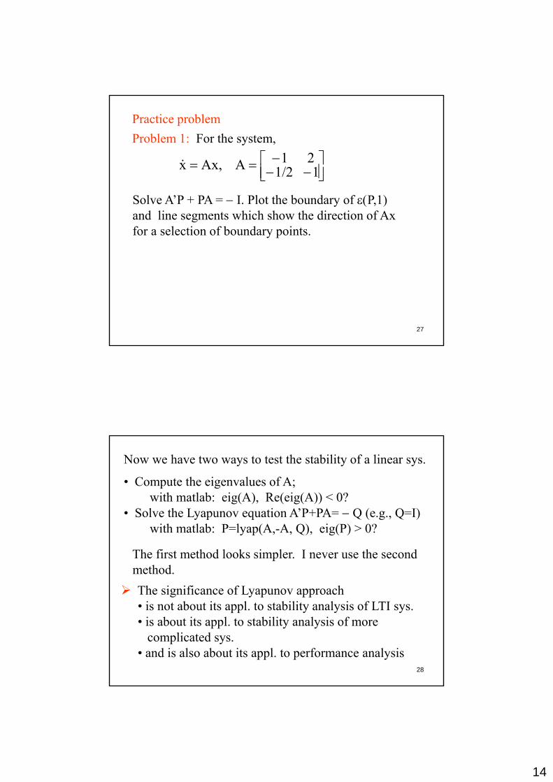
Practice problem

⎥⎦⎤

⎢⎣⎡

−−−== 11/2

21AAx,x

Problem 1: For the system,

⎦⎣

Solve A’P + PA = − I. Plot the boundary of ε(P,1) and line segments which show the direction of Axfor a selection of boundary points.

27

Now we have two ways to test the stability of a linear sys.

• Compute the eigenvalues of A;with matlab: eig(A), Re(eig(A)) < 0?

• Solve the Lyapunov equation A’P+PA= − Q (e.g., Q=I)y p q Q ( g , Q )with matlab: P=lyap(A,-A, Q), eig(P) > 0?

The first method looks simpler. I never use the secondmethod. The significance of Lyapunov approach

i t b t it l t t bilit l i f LTI

28

• is not about its appl. to stability analysis of LTI sys.• is about its appl. to stability analysis of more

complicated sys.• and is also about its appl. to performance analysis

15

Other applications:• The maximal output by bounded input. For the LTI sys,

(*) Cx yBu,Axx =+=

We only know that ||u(t)||2≤ k . Suppose x(0)=0.What is the maximal output ||y(t)||∞ ? This problem is formulated when u is a disturbance. Need to evaluate the effect of disturbances.

• The maximal output by a set of initial states.

29

The maximal output by a set of initial states.For (*), assume u=0. x(0)∈X. What is the maximal output ||y(t)||∞?

A simple performance measure: the convergence rate

Consider the zero-state response of

0xx(0):Axx == 0x x(0):Axx

Have x(t)=eAtx0. If the system is stable, then x(t) → 0 as t→∞.It is desirable that x(t) converges to zero as fast as possible.

• How to describe this property?

30

16

Definition: The convergence rate is defined as the maximal α such that there exists a constant c > 0 satisfying

Consider a stable system, Axx =

||x(t)||2 ≤ c ||x0|| e−αt for all x0∈Rn.

n1,2,...,i:(A))Re(λmax rate econvergenc The 2) i =−=

Theorem:1) The convergence rate is the maximal γ such that

there exists P=P’>0 satisfyingA’P + PA < -2 γ P

31

Note 2: The first property can be extended to more complicated systems when exact solution is unavailable.

Note 1: The convergence rate is also an index of stability margin.It indicates how far away the system is from being unstable.

Next we are going to deal withNext, we are going to deal with stability of

Linear Differential Inclusions

32

Note: Using the Lyapunov function method, LDI is onlyone step away from LTI.

17

Linear Differential Inclusions (LDIs)

Motivation: how does LDI arise?

Example: A system with uncertain parametersExample: A system with uncertain parameters )x,(t)Ak(t)Ak(Ax 22110 ++=

The parameters k1(t) and k2(t) are time-varying anduncertain. We only know that |k1(t)| ≤ 1 and |k2(t)| ≤ 1.Denote Ω:= Α0+k1A1+k2A2: |k1|≤1,|k2|≤1,

33

Ω is a subset of Rn×n, or a set of n×n real matrices.At every instant, we don’t know dx/dt exactly, except that

Ω∈∈ A :Axx An LDI

Example: A nonlinear system(Fx)BAxx ψ+=

ψ(.) is a scalar function.It is known but we don’t have

v

uk1

u

uk2 ψ(u)

suitable tools to handle suchkind of nonlinearity.If we bound ψ(.) with two linear functions k1u and k2u,then

]k,[kk :kFx(Fx) 21∈∈ψ

34

]k,[kk :kBFxAx(Fx)BAxx 21∈+∈+= ψIf we let Ω=A+kBF: k∈[k1,k2]. Again we have

ΩA :Axx ∈∈

18

nonlinear systems,uncertain systems,

Linear differential inclusions are used to describe complicated systems, such as

switched systems and time-varying systems

witha family of linear systems

• This makes a complicated s stem approachable

35

• This makes a complicated system approachable with tools extended from those for linear systems.

• We first review some concept about convex set.

Consider a vector space, e.g., Rp

(note Rn×m is also a vector space)

Let s1,s2∈Rp. The set ks + (1 k)s : k∈[0 1]

s2ks1+ (1-k)s2: k∈[0,1] represents a line segment between s1 and s2.

s1

Let S be a subset of Rp, i.e., S ⊆ Rp. S is said to be a convex set if for any two s1,s2∈ S,

36

ks1+ (1-k)s2: k∈[0,1] ⊆ S

s1

s2 Notconvex convex

19

Convex hull of a set of points

Let s1, s2, …, sN be a set of points in Rp. The convexhull of s1, s2, …, sN, denoted cos1, s2, …, sN, is theminimal convex set that includes s1, s2, …, sNminimal convex set that includes s1, s2, …, sN

s1s2 s3

s4

ss6

It is a polygon.

37

s5

⎭⎬⎫

⎩⎨⎧

≥=+++== ∑=

N

1iiN21iii 0α 1,α...αα :sαN,1,2,i :cos

A convex linear combination

Examples

(1,1)(-1,1)⎭⎬⎫

⎩⎨⎧

⎥⎦⎤

⎢⎣⎡−−

⎥⎦⎤

⎢⎣⎡−

⎥⎦⎤

⎢⎣⎡−⎥⎦

⎤⎢⎣⎡= 1

1,11,1

1,11co

⎬⎫

⎨⎧ ≤≤⎥

⎤⎢⎡= 1|k|1|k|:k1

(-1,-1) (1,-1)

(0,-1) (1,0)

(0,1)

⎭⎬⎫

⎩⎨⎧

⎥⎦⎤

⎢⎣⎡−⎥⎦

⎤⎢⎣⎡−

⎥⎦⎤

⎢⎣⎡

⎥⎦⎤

⎢⎣⎡= 1

0,01,1

0,01co

⎭⎬

⎩⎨ ≤≤⎥⎦⎢⎣

= 1|k| 1,|k| :k 212

⎬⎫

⎨⎧ ⎤⎡k1

1k:Rk 2 ≤∈=∞

38

(0,-1) ⎭⎬⎫

⎩⎨⎧ ≤+⎥⎦

⎤⎢⎣⎡= 1|k||k| :kk

212

1

1k:Rk1

2 ≤∈=

20

A system contains uncertain parameters:

)x,(t)Ak(t)Ak(Ax 22110 ++= (1,1)(-1,1)

k1

k2

Each point (k1, k2) corresponds to a matrix

(k k ) A k E k E (-1,-1) (1,-1)(k1,k2) → A0+k1E1+k2E2

This defines a map from R2 to Rn×n. It is an affine map

Let S be a polygon in R2 with vertices s1, s2, …, sN, S=cos1,s2,…

Denote Ω =A0+k1E1+k2E2: [k1 k2]’∈S (the image of S)

39

Ω is a polygon in Rn×n. A vertex of S corresponds to a vertex of Ω.

Ω = coA0+k1E1+k2E2: [k1 k2]’=s1, s2,…sN

Examples

4321 A,A,A,Aco= 1|k| 1,|k| :EkEkA 21221101 ≤≤++=Ω

EEAAEEAA −+=++=

(1,1)(-1,1)

(1 1).EEAA ,EEAA ,EEAA ,EEAA

21042103

21022101

−−=+−=−+=++=

1|k|1,|k| 1,|k| :EkEkEkA 32133221102 ≤≤≤+++=Ω

87654321 A,A,A,A,A,A,A,Aco=

EEEAAEEEAA ++=+++=

(-1,-1) (1,-1)

40

,EEEAA ,EEEAA ,E-EEAA ,EEEA,EEEAA ,EEEAA ,E-EEAA ,EEEAA

3210832107

3210632105

3210432103

3210232101

−−−=+−−=+−=++−=

−−+=+−+=++=+++=

A

21

Examples

4321 A,A,A,Aco=

1|k| |k| :EkEkA 21221103 ≤+++=Ω

(0,-1)

(0,-1) (1,0)

(0,1)

.EAA ,EAA ,EAA ,EAA

204203

102101

−=+=−=+=

1|k||k||k| :EkEkEkA 32133221104 ≤+++++=Ω

654321 A,A,A,A,A,Aco=

41

,EAA ,EA,EAA ,EAA ,EAA ,EAA

306305

204203

102101

−=+=−=+=−=+=

A

Stability of Polytopic LDIsGiven a set of n×n real matrices A1, A2, …AN.Let Ω=coA1,A2,…,AN. Consider the LDI

ΩA:Axx ∈∈ ΩA :Axx ∈∈

Theorem: The LDI is stable if there exists P=P’>0such that

xAx,...,Ax,Acox ly,Equivalent N21∈

42

0'

0'0'

22

11

<+

<+<+

NN PAPA

PAPAPAPA

22

Main idea: Consider the ellipsoid ε(P,r). Let x0 be a point on its boundary.

A1’P+PA1< 0 ⇒ ⟨ Px0, A1x0⟩ < 0

A ’P+PA < 0 ⇒ ⟨ Px A x ⟩ < 0

Px0

A2x0A

x0

A2 P+PA2< 0 ⇒ ⟨ Px0, A2x0⟩ < 0

AN’P+PAN< 0 ⇒ ⟨ Px0, ANx0⟩ < 0

…

N21

N21N21

and 1,... t.s. 0,,...,, x,x,...AAx,coAx Since

αααααα

=+++≥∃∈

A1x0ANx0

43

0NN022011x xA...xAxA|x0

ααα +++=

0xA,Px|x,PxN

1i0i0x0 0

<= ∑=

This is valid for all x on the boundary of each ellipsoid.A trajectory will enter smaller and smaller ellipsoids.

Definition: The convergence rate αmax is defined as the maximal α such that there exists constant c > 0 satisfying

The convergence rate for an LDI

||x(t)||2 ≤ c ||x0|| e−αt

Theorem: Let γmax be the maximal γ such that there exists P=P’>0 satisfying

for all x0∈Rn and all possible solutions x(t) corresponding to each x0.

P 2γPAP'AP 2γPAP'A

22

11

−<+−<+

44

P 2γPAP'A

NN −<+

Then γmax≤ αmax.

We can use γmax as an estimate for the convergence rate.If γmax > 0, then the LDI is stable.

23

The optimization problem for computing the maximal γmax

P 2γPAP'A P 2γPAP'A t.s.

γsup

22

11

−<+−<+

Linear matrix inequalitiesC b ffi i tl l d

IP'P P 2γPAP'A

NN

>=−<+

Can be efficiently solved with Matlab

45

Example:

[0,1.2]g(t) ,0110g(t)25.1

11 ∈⎟⎠⎞

⎜⎝⎛

⎥⎦⎤

⎢⎣⎡−

−+⎥⎦⎤

⎢⎣⎡

−−−= xx

A second-order system with an uncertain/time-varyingparameter g

The system can be described with the following LDI

⎥⎦⎤

⎢⎣⎡

−−−−=⎥⎦

⎤⎢⎣⎡

−−−=∈ 27.2

2.01A ,25.111A ,xAx,Acox 2121

γsupUsing LMI solver, the solution to

46

IP'P P 2γPAP'A P2γPAP'A t.s.

22

11

>=−<+−<+

⎥⎦⎤

⎢⎣⎡=>= 2.29882.8735

2.873512.0687P ,06051.0 γis

24

⎥⎦⎤

⎢⎣⎡

−−−−=⎥⎦

⎤⎢⎣⎡

−−−=∈ 27.2

2.01A ,25.111A ,xAx,Acox 2121

⎥⎦⎤

⎢⎣⎡=>= 2.29882.8735

2.873512.0687P ,06051.0γ

The system is stable To demonstrate this result we plot theThe system is stable. To demonstrate this result, we plot theverctor A1x and A2x along the boundary of ε(P,1)

0.4

0.6

0.8

0.4

0.6

0.8

A1xA2x

47-0.4 -0.3 -0.2 -0.1 0 0.1 0.2 0.3 0.4-0.8

-0.6

-0.4

-0.2

0

0.2

-0.4 -0.3 -0.2 -0.1 0 0.1 0.2 0.3 0.4-0.8

-0.6

-0.4

-0.2

0

0.2

Stability for discrete-time systems

Consider a system: x[k+1]=f(x[k])

Given a quadratic function V(x)=x’Px.

*

*

**•

•

•

•

x[k]

x[k+1]

Theorem: The system is stable if

f(x)’P f(x) < x’Px for all x≠0. (1)

Interpretation: • Consider x[k] on the boundary of an ellipsoid: x[k]∈∂ ε(P r)

48

• Consider x[k] on the boundary of an ellipsoid: x[k]∈∂ ε(P,r), i.e. x[k]’Px[k]= r.

• Condition (1) implies that x[k+1]’P x[k+1] < r, ⇒ x[k+1] is inside the ellipsoid. A trajectory will go to smaller and smaller ellipsoid. ⇒ stable

25

Stability for LTI systems

Consider a system: x[k+1]=Ax[k]

Given a quadratic function V(x)=x’Px.

*

*

**•

•

•

•

x[k]

x[k+1]

Theorem: The system is stable if

A’P A < P (2)

Note that (2) implies that ’A’PA < ’P ⇒ [k+1]’P [k+1] < [k] P [k]

49

x’A’PAx < x’Px ⇒ x[k+1]’Px[k+1] < x[k] P x[k]

Theorem: The following are equivalentThere exists P=P’>0 satisfying (2)All eigenvalues of A are within the unit disk, i.e., |λi|<1 for all i.

Stability of Polytopic LDIsGiven a set of n×n real matrices A1, A2, …AN.Let Ω=coA1,A2,…,AN. Consider the LDI (linear difference inclusion)Co s de e ( ea d e e ce c us o )

ΩA :Ax[k]1]x[k ∈∈+

Theorem: The LDI is stable if there exists P=P’>0such that

x[x]Ax[k],...,Ax[k],Aco1] x[kly,Equivalent N21∈+

50

such that

0PPA'A

0PPA'A0PPA'A

NN

22

11

<−

<−<−

26

Definition: The convergence rate βmin is defined as the minimal β > 0 such that there exists constant c > 0 satisfying

The convergence rate for an LDI

||x[k]||2 ≤ c ||x0|| βk

Theorem: Let γmin be the minimal γ > 0 such that there exists P=P’>0 satisfying

for all x0∈Rn and all possible solutions x[k] corresponding to each x0.

0P γPA'A0P γPA'A

22

11

<−<−

51

0P γPA'A NN <−

Then γmin > βmin.

We can use γmin as an estimate for the convergence rate.If γmin < 1, then the LDI is stable.

Final Exam Coverage:

Matrix functions: eAt, Ak, when A has complex eigenvalues orrepeated eigenvalues

Solution to LTI systems, stability Realization of transfer functionsControllability and observabilityControllability/observability decomposition State feedback design: two approaches Observer design: two approaches

M tl b/Si li k bl

52

Matlab/Simulink problems• Feedback from estimated states• Robust tracking and disturbance rejection• LQR optimal control

27

DuCxyBu;Axx +=+=Consider the system:

Given x(0) and u(t) for t ≥ 0. The solution ist )A(A ∫

Solution to a LTI system, stability, time response

Du(t))d(BuCex(0)Cey(t)

;)d(Buex(0)ex(t)t

0

τ)A(tAt

t

0

τ)A(tAt

++=

+=

∫∫

−

−

ττ

ττ

Re(λi) <0, for all .i, then as t → ∞, all terms converges to 0, eAt→ 0, x(t) always converges to 0. → Stable system.Re(λi) > 0, for some .i, then as t → ∞, some terms diverge.

53

There exist x0 such that x(t) grows unbounded. Unstable Re(λi) ≤ 0 for all .i, all eigenvalues with 0 real parts are simple, eAt is bounded for all t but not converge to 0. critical caseRe(λi) ≤ 0 for all .i, some eigenvalues with 0 real parts are repeated, eAt unbounded; x(t) unbounded for some x0. unstable

[ ]

r1r1r

1r

nmir1r

2r2

1r1

asasasd(s)

RN),G(NsNsNsNd(s)

1G(s)

++++=

∈∞+++++=

−−

×−

−−

Realization of transfer function

Th li ti f G ( ) i iThe realization of Gsp(s) is given as:

⎥⎥⎥⎥

⎦

⎤

⎢⎢⎢⎢

⎣

⎡

=

⎥⎥⎥⎥⎥

⎦

⎤

⎢⎢⎢⎢⎢

⎣

⎡ −−−−

=

−

0000

,

0I00

00I0000I

IaIaIaIa

A

p

p

p

prp1rp2p1pI

B

54

[ ] )G(D ,NNNNC r1r21 ∞== −

28

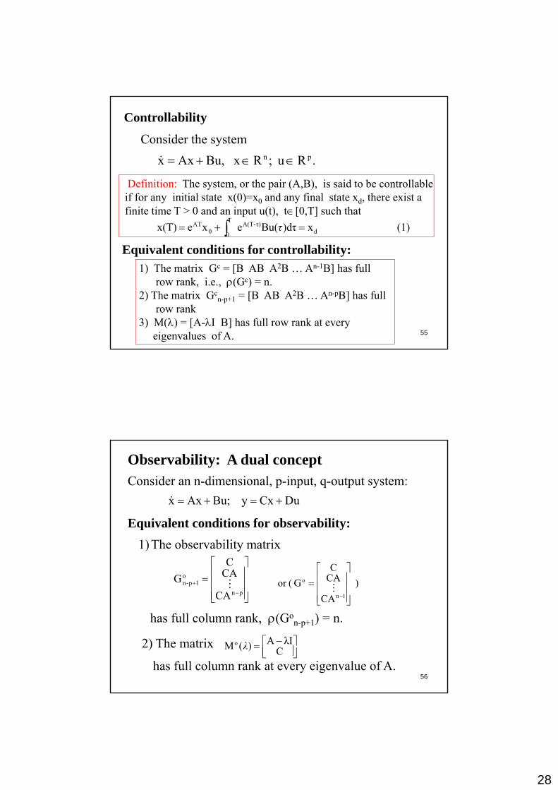
Controllability

Consider the system.Ru ;R xBu,Axx pn ∈∈+=

D fi i i Th h i (A B) i id b ll blDefinition: The system, or the pair (A,B), is said to be controllable if for any initial state x(0)=x0 and any final state xd, there exist a finite time T > 0 and an input u(t), t∈[0,T] such that

(1) x)dτBu(exex(T) dτ)-A(TT

00AT =+= ∫ τ

Equivalent conditions for controllability:1) Th i G [B AB A2B A 1B] h f ll

55

1) The matrix Gc = [B AB A2B … An-1B] has full row rank, i.e., ρ(Gc) = n.

2) The matrix Gcn-p+1 = [B AB A2B … An-pB] has full

row rank3) M(λ) = [A-λI B] has full row rank at every

eigenvalues of A.

Observability: A dual conceptConsider an n-dimensional, p-input, q-output system:

DuCxy Bu;Axx +=+=

Equivalent conditions for observability:Equivalent conditions for observability:1) The observability matrix

⎥⎥⎥

⎦

⎤

⎢⎢⎢

⎣

⎡=

−+

pn

o1p-n

CA

CAC

G ) CA

CAC

G (or 1n

o

⎥⎥⎥

⎦

⎤

⎢⎢⎢

⎣

⎡=

−

56

has full column rank, ρ(Gon-p+1) = n.

2) The matrix ⎥⎦⎤

⎢⎣⎡ −= C

λIA)(Mo λ

has full column rank at every eigenvalue of A.

29

Controllability decomposition

Recall Gc=[B AB … An-1B]. Suppose that ρ(Gc) = n1 < n. Then Gc has at most n1 LI columns.They form a basis for the range space of Gc.

Theorem: Suppose that ρ(Gc) = n1 < n. Let Q be a nonsingular matrix whose first n1 columns are LI columns of Gc. Let P=Q-1. Then

[ ]

pnc

nnc

c

c

12c1

CCC

RB,RA,0BPBB,

A0AAPAPA 111

=

∈∈⎥⎦⎤

⎢⎣⎡==⎥

⎦

⎤⎢⎣

⎡== ××−

57

[ ]cc CCC =

DBA)C(sIDB)A(C and lecontrollab is )B,A(pair theMoreover,

1c

1cc

cc

+−=+− −−sI

Theorem: Suppose that ρ(Go) = n1 < n Let P be a nonsingular

Observability decomposition (follows from duality)

⎥⎥⎥

⎦

⎤

⎢⎢⎢

⎣

⎡=

−1n

o

CA

CAC

G Recall

Theorem: Suppose that ρ(G ) n1 < n. Let P be a nonsingular matrix whose first n1 rows are LI rows of Go. Then

[ ] 1

111

noo

pno

nno

o

o

o21

o1

RC ,0CC

RB,RA,BBPBB,

AA0APAPA

×

××−

∈=

∈∈⎥⎦

⎤⎢⎣

⎡==⎥⎦

⎤⎢⎣

⎡==

q

DBA)C( IDB)A(C and observable is )C,A(pair theMoreover,

11oo

−−I

58

DBA)C(sIDB)A(C 1o

1oo +−=+− −−sI

30

Controllable Canonical Form

234A)d ( I

Theorem: Suppose that (A,b) is controllable and

For simplicity, we consider a 4th-order system. The results forthe general case can be easily extended from the pattern.

432

23

14 αsαsαsαsA)det(sI ++++=−

[ ]⎥⎥⎥

⎦

⎤

⎢⎢⎢

⎣

⎡

==

1000α100αα10ααα1

bAbAAbbP:QLet 1

21

321

321-

With the state transformation z = Px, we have

43211- 0

1Pbb0001

ααααPAPA ⎥

⎥⎤

⎢⎢⎡

==⎥⎥⎤

⎢⎢⎡ −−−−

==Controllable

59

[ ]43211 ββββcPc

,00Pbb,

01000010PAPA

==⎥⎥⎦⎢

⎢⎣

==⎥⎥⎦⎢

⎢⎣

==

−

Furthermore, 43

22

31

443

22

311

αsαsαsαsβsβsβsβb)A(sIc++++

+++=− −

Canonical form

Pole assignment for state feedback: first approach via controllable canonical form

Step 1. Choose the desired eigenvalue set λi, i=1,2,…n which contains conjugate complex pairs, e.g., λi = -1+j2 and λi+1= −1−j2 and obtain the coefficients of

n1n1n

1nn

21d αsαsαs)λ(s)λ)(sλ(s(s) ++++=−−−=Δ −−

Step 2. Compute the characteristic polynomial of A

n1n1n

1n αsαsαsA)sIdet((s) ++++=−=Δ −

−

and the transformation matrix, e.g., for n = 4

60

[ ] ,

1000α100αα10ααα1

bAbAAbbP:Q1

21

321

321-

⎥⎥⎥

⎦

⎤

⎢⎢⎢

⎣

⎡

==

31

,0001

Pbb,010000100001αααα

PAPAThen 4321

1-

⎥⎥⎥

⎦

⎤

⎢⎢⎢

⎣

⎡==

⎥⎥⎥

⎦

⎤

⎢⎢⎢

⎣

⎡ −−−−

==

⎥⎤

⎢⎡ −−−−−−−− kαkαkαkα 44332211

⎥⎥⎥

⎦⎢⎢⎢

⎣

=

010000100001kb-A

Step 3: iii αα k Choose −=

⎥⎥⎤

⎢⎢⎡ −−−−

= 0001ααα

kb-AThen4321α

61

⎥⎥⎦⎢

⎢⎣

=

01000010kb-AThen

Step 4: P. kk Compute =

n1,2,...,i,λ seigenvalue desired thehas )QkbAQ(bk-Athen

i

1

=−= −

– Select F having desired closed-loop eigenvalues which are different from those of A

– Choose an arbitrary K0 such that F,K0 is observable– Solve AT-TF=BK0 to obtain the unique T

Second approach via solving matrix equations

Solve AT-TF BK0 to obtain the unique T.

T=lyap(A,-F,-B*K0)

– If T is non-singular, let K = K0 T-1. Then A-BK has the desired eigenvalues.

– If T is singular, which is rarely the case,

62

choose a different K0 and try again

– Finally, check if A-BK has the desired eigenvalues.

eig(A-B*K)=?

32

Full Dimensional State Estimator

Theorem. If a SISO system is observable, then it can be transformed, by an equivalent transformation, to an observable canonical form

• Obser able Canonical Form:

[ ] dux1..000y;u:

x

100:::::

..010

..001

..000

x

1

2n

1n

n

1

2n

1n

n

+=

⎥⎥⎥⎥⎥⎥

⎦

⎤

⎢⎢⎢⎢⎢⎢

⎣

⎡

β

βββ

+

⎥⎥⎥⎥⎥⎥

⎦

⎤

⎢⎢⎢⎢⎢⎢

⎣

⎡

α−

α−α−α−

= −

−

−

−

• Observable Canonical Form:

63

1..00 11 ⎥⎦⎢⎣ β⎥⎦⎢⎣ α

A procedure for assigning the eigenvalues for A-LC can bederived from the observable canonical form.

For mu

Second approach via solving matrix equations

Let A, C be given.

The procedure:• Pick F having desired eigenvalues. • Pick L0 and solve TA − FT = L0C for T. • If T is nonsingular, let L=T-1L0. • Then A − LC has the desired eigenvalues.

64

33

Matlab/Simulink problems

• Feedback from estimated states• Robust tracking and disturbance rejection• LQR optimal control

65