16.360 Lecture 9

Special cases

= |V0| [1+ | |² + 2||cos(2z + r)] + 1/2

|V(z)|

1. ZL= Z0, = 0

= |V0| +|V(z)|

2. ZL= 0, short circuit, = -1

|V(z)|

|V0| +

- -3/4 -/2 -/4

= |V0| [2 + 2cos(2z + )] + 1/2

|V(z)|

|V(z)|

2|V0| +

- -3/4 -/2 -/4

Standing Wave

3. ZL= , open circuit, = 1

= |V0| [2 + 2cos(2z )] + 1/2

|V(z)|

|V(z)|

2|V0| +

- -3/4 -/2 -/4

-V0

+V0=

ZL Z0-

ZL Z0+

16.360 Lecture 9

short circuit line

ZL= 0, = -1, S =

Vg(t) VL

A

z = 0

B

l

ZL = 0

z = - l

Z0

ZgIi

Zinsc

i(z) =

V(z) = V0 )- ejz

+

(e-jz

(e-jz+

V0

Z0 ejz )

= -2jV0sin(z)+

= 2V0cos(z)/Z0+

Zin =V(-l)

i(-l)= jZ0tan(l)

16.360 Lecture 9

open circuit line

ZL = , = 1, S =

Vg(t) VL

A

z = 0

B

l

ZL =

z = - l

Z0

ZgIi

Zinoc

i(z) =

V(z) = V0 )+ ejz

-

(e-jz

(e-jz+

V0

Z0 ejz )

= 2V0cos(z)+

= 2jV0sin(z)/Z0+

Zin =V(-l)

i(-l)= -jZ0cot(l)

oc

Short-Circuit/Open-Circuit Method• For a line of known length l, measurements of its input

impedance, one when terminated in a short and another when terminated in an open, can be used to find its characteristic impedance Z0 and electrical length

16.360 Lecture 9

16.360 Lecture 9

Line of length l = n/2

tan(l) = tan((2/)(n/2)) = 0,

Any multiple of half-wavelength line doesn’t modify the load impedance.

= ZLZin

16.360 Lecture 9

Quarter-wave transformer l = /4 + n/2

= Z0²/ZL

l = (2/)(/4 + n/2) = /2 ,

+(1 e-j2l )

-(1 e-j2l )

Z0Zin(-l) =+(1 e

-j )

-(1 e-j

)Z0=

(1 + ) Z0(1 - )

=

16.360 Lecture 9

An example:

A 50- lossless tarnsmission is to be matched to a resistive load impedance with ZL = 100 via a quarter-wave section, thereby eliminating reflections along the feed line. Find the characteristic impedance of the quarter-wave tarnsformer.

ZL = 100

/4

Z01 = 50

Zin = Z0²/ZL= 50

Z0 = (ZinZL) = (50*100)½ ½

= Z0²/ZLZin

16.360 Lecture 9

Matched transmission line:

1. ZL = Z0

2. = 03. All incident power is delivered to the load.

16.360 Lecture 9

• Instantaneous power• Time-average power

i(z) =

V(z) = V0 ( )

+V0

Z0

At load z = 0, the incident and reflected voltages and currents:

V = V0+ i =

i i

V = V0-r

i = -

V0

Z0

r

++e jz

-

e-jz

ejz )(e-jz+

V0

Z0

16.360 Lecture 9

• Instantaneous power

+

iP(t) = v(t) i(t) = Re[V exp(jt)] Re[ i exp(jt)] i i

= Re[|V0|exp(j )exp(jt)] Re[|V0|/Z0 exp(j )exp(jt)] + + +

= (|V0|²/Z0) cos²(t + ) + +

-

rP(t) = v(t) i(t) = Re[V exp(jt)] Re[ i exp(jt)] r r

= Re[|V0|exp(j )exp(jt)] Re[|V0|/Z0 exp(j )exp(jt)] + - +

= - ||²(|V0|²/Z0) cos²(t + + r) + +

16.360 Lecture 9

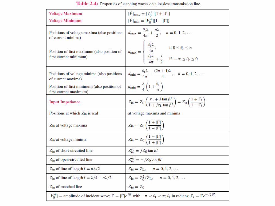
• Time-average

(|V0|²/Z0) cos²(t + )dt + +

Time-domain approach:

Pav =i

T1

0

TP (t)dt

i= 2

0

T

= (|V0|²/2Z0)+

Pavr

= -||² (|V0|²/2Z0)+

= PaviPav + Pav

r

= (1-||²) (|V0|²/2Z0)+

Net average power:

16.360 Lecture 9

• Time-average

Phasor-domain approach

Pavr

= -||² (|V0|²/2Z0)+

= (1-||²) (|V0|²/2Z0)+

= (½)Re[V i*]Pav

Pav = (1/2) Re[V0 V0* /Z0]i + +

= (|V0|²/2Z0)

Pav

+

Lumped element model

TL effect

l/>0.01 Vg(t) VBB’(t)VAA’(t)

A

A’ B’

B

z z z

Vg(t)

R’z L’z

G’z C’z

R’z L’z

G’z

R’z

C’z

L’z

G’z

C’z

TL Equation Wave Equation

Solution of Wave Equation

Lossless TLReflection coefficient

Standing WaveWave (Input) Impedance

Solving for V0 + Complete

Solution

Power

+