U.S. Department of Energy FreedomCAR and Vehicle Technologies, EE-2G

1000 Independence Avenue, S.W. Washington, D.C. 20585-0121

FY 2007 16,000-RPM INTERIOR PERMANENT MAGNET RELUCTANCE MACHINE WITH BRUSHLESS FIELD EXCITATION Prepared by: Oak Ridge National Laboratory Mitch Olszewski, Program Manager

Submitted to: Energy Efficiency and Renewable Energy FreedomCAR and Vehicle Technologies Vehicle Systems Team Susan A. Rogers, Technology Development Manager October 2007

ORNL/TM-2007/167

Engineering Science and Technology Division

16,000-rpm Interior Permanent Magnet Reluctance Machine with Brushless Field

Excitation

J. S. Hsu T. A. Burress

S. T. Lee R. H. Wiles

C. L. Coomer J. W. McKeever

D. J. Adams

Publication Date: October 2007

Prepared by the OAK RIDGE NATIONAL LABORATORY

Oak Ridge, Tennessee 37831 managed by

UT-BATTELLE, LLC for the

U.S. DEPARTMENT OF ENERGY Under contract DE-AC05-00OR22725

DOCUMENT AVAILABILITY

Reports produced after January 1, 1996, are generally available free via the U.S. Department of Energy (DOE) Information Bridge:

Web site: http://www.osti.gov/bridge Reports produced before January 1, 1996, may be purchased by members of the public from the following source:

National Technical Information Service 5285 Port Royal Road Springfield, VA 22161 Telephone: 703-605-6000 (1-800-553-6847) TDD: 703-487-4639 Fax: 703-605-6900 E-mail: info@ntis.fedworld.gov Web site: http://www.ntis.gov/support/ordernowabout.htm

Reports are available to DOE employees, DOE contractors, Energy Technology Data Exchange (ETDE) representatives, and International Nuclear Information System (INIS) representatives from the following source:

Office of Scientific and Technical Information P.O. Box 62 Oak Ridge, TN 37831 Telephone: 865-576-8401 Fax: 865-576-5728 E-mail: reports@osti.gov Web site: http://www.osti.gov/contact.html

This report was prepared as an account of work sponsored by an agency of the United States Government. Neither the United States government nor any agency thereof, nor any of their employees, makes any warranty, express or implied, or assumes any legal liability or responsibility for the accuracy, completeness, or usefulness of any information, apparatus, product, or process disclosed, or represents that its use would not infringe privately owned rights. Reference herein to any specific commercial product, process, or service by trade name, trademark, manufacturer, or otherwise, does not necessarily constitute or imply its endorsement, recommendation, or favoring by the United States Government or any agency thereof. The views and opinions of authors expressed herein do not necessarily state or reflect those of the United States Government or any agency thereof.

ii

CONTENTS

Page

LIST OF FIGURES .............................................................................................................................. iii LIST OF TABLES................................................................................................................................ v ACRONYMS........................................................................................................................................ vi INTRODUCTION ................................................................................................................................ 1 PROTOTYPE MOTOR ……………………………………………………………………………… 2 AIR GAP FLUX, INDUCTANCE, PERFORMANCE PARAMETER COMPUTATIONS,

AND COMPARISONS OF SIMULATION WITH TEST RESULTS…………………..…… 6 MECHANICAL STRESS COMPUTATIONS .................................................................................... 15 BACK-EMF TESTS ………………………………………………………………………………..... 17 CORE/FRICTION LOSS TESTS…………………………................................................................. 20 LOCKED ROTOR TESTS ……………………………………………………………………… ...... 23 PERFORMANCE/EFFICIENCY TESTS ………………………………………………………… ... 25 REWOUND MOTOR TESTS………………………………………………………............................ 30 BACK-EMF RESULTS........................................................................................................................ 31 NO-LOAD LOSS DATA ..................................................................................................................... 32 EFFICIENCY MAPPING .................................................................................................................... 34 VIBRATION ANALYSIS ………………………………………………………… ........................... 42 CONCLUSIONS................................................................................................................................... 43 REFERENCES ..................................................................................................................................... 45 APPENDIX: ADDITIONAL SECOND SERIES TEST EFFICIENCY MAPS OF 16,000-RPM RIPM BFE REWOUND MOTOR ........................................................................ 46

iii

LIST OF FIGURES Figure Page

1 Assembly of ORNL 16,000-rpm motor design .................................................................... 2 2 Location of bridge in a rotor punching ................................................................................. 3 3 Flexibility provided by adjustable field excitation .............................................................. 3 4 Rotor CAD drawing of ORNL’s 16,000-rpm motor ............................................................ 4 5 Wound stator core................................................................................................................. 4 6 Rotor punching ..................................................................................................................... 4 7 Rotor core stack and shaft..................................................................................................... 5 8 Completed rotor.................................................................................................................... 5 9 Excitation coil housing ......................................................................................................... 5 10 Excitation coil inside the coil housing.................................................................................. 5 11 Air-gap flux density distributions for various field excitations ............................................ 6 12 Expected motor torque vs. load angle at Imax = 200 A for different field excitations ........... 7 13 Simulated results of a phase back-emf at Iexc = 5000 AT and 5000 rpm .............................. 7 14 Calculated back-emf voltages of 16,000-rpm motor ............................................................ 8 15 Inductances vs. current angle at 100 Arms phase current....................................................... 9 16 Inductances vs. current values .............................................................................................. 9 17 Simulated phasor diagram of the simple 6000 rpm RIPM motor with side PMs at 3500 rpm and 233Vrms ...................................................................................................... 10 18 Simulated phasor diagram of the simple 6000 rpm RIPM motor with side PMs at 3500 rpm and 100 Arms ..................................................................................................... 11 19 Saturated inductance values of 16,000-rpm motor vs. current angle at Iph, = 100 A rms ........ 12 20 Saturated lined-up inductance values of 16,000-rpm motor vs. current values.................... 12 21 Simulated phasor diagram of 16,000-rpm IPM SM at 3,300 rpm, 5 A excitation, and 270 Vrms.......................................................................................................................... 13 22 Simulated phasor diagram of 16,000-rpm IPM SM at 3,300 rpm, 5 A excitation, and 100 A rms ......................................................................................................................... 13 23 Finite element stress analysis of 16,000-rpm rotor............................................................... 15 24 Radial displacement of the 16,000-rpm rotor ....................................................................... 16 25 Shear stresses at the support columns of an 0.018-in. thick 16,000-rpm laminate rotor ...... 16 26 Unloaded phase back-emf baseline waveforms (16.3 Vrms @ 1000 rpm) ............................ 17 27 Unloaded phase back-emf waveforms enhanced with 5 A of field current (38 Vrms @ 1000 rpm)........................................................................................................... 17 28 Influence of field current on unloaded back-emf curves ...................................................... 18 29 Influence of field current on unloaded back-emf phase voltage........................................... 18 30 Influence of field excitation current on torque needed to overcome unloaded core and

friction losses………………………………………………………………………………. 20 31 Influence of field excitation current on unloaded core and friction losses ........................... 21 32 Influence of field current on core losses............................................................................... 22 33 Locked rotor torque for the RIPM-BFE motor..................................................................... 23 34 Locked rotor torque with 5A field excitation current ........................................................... 24 35 Impact of flux saturation on peak torque.............................................................................. 24 36 Efficiency contours for the RIPM-BFE motor with no field excitation current ................... 25 37 Efficiency contours with 5A field excitation current excluding resistive losses of the BFE field coil.................................................................................................................. 26 38 Efficiency contours including 5A resistive losses of the BFE field coil .............................. 26

iv

LIST OF FIGURES (Continued)

Figure Page 39 Baseline (no field excitation current) efficiency contour map scaled for comparison with the contour map measured using 5A field excitation current ................... 27

40 Greater efficiency plot from efficiency contour maps for 0A and 5A field excitation currents showing how field excitation may be used to improve efficiency contours ............................................................................................................... 27

41 RIPM BFE efficiency map with high speed gear ratio of 2.6............................................... 28 42 Baseline (Prius motor) efficiency map ................................................................................. 28 43 Stator before (left) and after (right) rewinding ..................................................................... 30 44 Back-emf voltage vs. speed for both stators ......................................................................... 31 45 Required torques for spinning rotor vs. rotor speed at various field currents....................... 32 46 Spinning powers vs. rotor speed at different field currents .................................................. 32 47 Spinning losses vs. field current for various rotor speeds. ................................................... 33 48 16,000-rpm RIPM BFE efficiency contours with 5A field without field losses .................. 34 49 Efficiency contours using optimal field currents – without field losses ............................... 35 50 Optimal field currents – without field losses ........................................................................ 35 51 Efficiency contours for 90% without field losses for all field currents ................................ 36 52 Efficiency contours with 5A field – including field losses................................................... 37 53 Efficiency contours using optimal field current – including field losses.............................. 37 54 Optimal field currents when including field losses .............................................................. 38 55 Efficiency contours for 90% with field losses for all field currents ..................................... 38 56 Torque-current ratio for tests 1 and 2 at 5A.......................................................................... 39 57 Projected efficiency contours using optimal field current with field losses included .......... 40 58 RIPM BFE efficiency map with field losses and gear ratio of 2.6 ....................................... 41 59 Projected RIPM BFE efficiency map with field losses and gear ratio of 2.6 ....................... 41 60 Vibration analysis obtained from test ................................................................................... 42 61–62 Efficiency maps without field losses included ..................................................................... 46 63–64 Efficiency maps without field losses included ..................................................................... 47 65–66 Efficiency maps without field losses included ..................................................................... 48 67 Efficiency maps without field losses included ..................................................................... 49 68 Efficiency maps with field losses included .......................................................................... 49 69–70 Efficiency maps with field losses included .......................................................................... 50 71–72 Efficiency maps with field losses included .......................................................................... 51 73–74 Efficiency maps with field losses included .......................................................................... 52

v

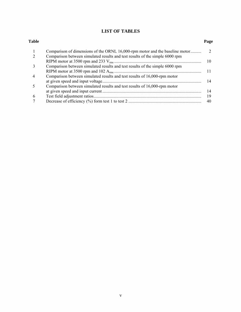
LIST OF TABLES Table Page

1 Comparison of dimensions of the ORNL 16,000-rpm motor and the baseline motor.......... 2 2 Comparison between simulated results and test results of the simple 6000 rpm RIPM motor at 3500 rpm and 233 Vrms ................................................................................ 10 3 Comparison between simulated results and test results of the simple 6000 rpm RIPM motor at 3500 rpm and 102 Arms ................................................................................ 11 4 Comparison between simulated results and test results of 16,000-rpm motor at given speed and input voltage........................................................................................... 14 5 Comparison between simulated results and test results of 16,000-rpm motor

at given speed and input current ........................................................................................... 14 6 Test field adjustment ratios................................................................................................... 19 7 Decrease of efficiency (%) form test 1 to test 2 ................................................................... 40

vi

ACRONYMS

3-D three dimensional A amperes of current ac alternate current AT ampere turns BFE brushless field excitation d-axis direct-axis dc direct current emf electromotive force ksi kilo-pounds per square inch Iexc field coil excitation in ampere turns Imax maximum stator winding current amplitude IPM interior permanent magnet Nm Newton meter ORNL Oak Ridge National Laboratory Pexc power loss of excitation coils PM permanent magnet PMSM permanent magnet synchronous motor q-axis quadrature-axis rms root mean square RIPM reluctance interior permanent magnet motor rpm revolutions per minute SM synchronous motor Vexc dc voltage fed to excitation coils

1

INTRODUCTION The reluctance interior permanent magnet (RIPM) motor is currently used by many leading auto manufacturers for hybrid vehicles. The power density for this type of motor is high compared with that of induction motors and switched reluctance motors. The primary drawback of the RIPM motor is the permanent magnet (PM) because during high-speed operation, the fixed PM produces a huge back electromotive force (emf) that must be reduced before the current will pass through the stator windings. This reduction in back-emf is accomplished with a significant direct-axis (d-axis) demagnetization current, which opposes the PM’s flux to reduce the flux seen by the stator wires. This may lower the power factor and efficiency of the motor and raise the requirement on the alternate current (ac) power supply; consequently, bigger inverter switching components, thicker motor winding conductors, and heavier cables are required. The direct current (dc) link capacitor is also affected when it must accommodate heavier harmonic currents. It is commonly agreed that, for synchronous machines, the power factor can be optimized by varying the field excitation to minimize the current. The field produced by the PM is fixed and cannot be adjusted. What can be adjusted is reactive current to the d-axis of the stator winding, which consumes reactive power but does not always help to improve the power factor. The objective of this project is to avoid the primary drawbacks of the RIPM motor by introducing brushless field excitation (BFE). This offers both high torque per ampere (A) per core length at low speed by using flux, which is enhanced by increasing current to a fixed excitation coil, and flux, which is weakened at high speed by reducing current to the excitation coil. If field weakening is used, the dc/dc boost converter used in a conventional RIPM motor may be eliminated to reduce system costs. However, BFE supports a drive system with a dc/dc boost converter, because it can further extend the constant power speed range of the drive system and adjust the field for power factor and efficiency gains. Lower core losses at low torque regions, especially at high speeds, are attained by reducing the field excitation. Safety and reliability are increased by weakening the field when a winding short-circuit fault occurs, preventing damage to the motor. For a high-speed motor operating at 16,000-revolutions per minute (rpm), mechanical stress is a challenge. Bridges that link the rotor punching segments together must be thickened for mechanical integrity; consequently, increased rotor flux leakage significantly lowers motor performance. This barrier can be overcome by BFE to ensure sufficient rotor flux when needed.

2

PROTOTYPE MOTOR A CAD assembly cross section of the Oak Ridge National Laboratory (ORNL) 16,000-rpm motor design is shown in Fig. 1.

Fig. 1. Assembly of ORNL 16,000-rpm motor design.

Table 1 compares the dimensions of the ORNL 16,000-rpm motor with those of the Toyota/Prius motor [1,2] that was selected as a base line motor. The masses and sizes derived from this table provide a basis for a cost comparison. The extra excitation coils and cores of the ORNL motor are made of copper wires and mild steel, respectively. Cost savings can be realized by having a shorter stator core (1.88 inches vs. 3.3 inches) as well as shorter stator windings. The cost of the 5 A maximum low current control of the field excitation is minimal because of the low current component requirements. This design approach enables better motor performance as well as system cost savings. Additionally, if used in a vehicle architecture having a boost converter, the output of this motor design can be further increased.

Table 1. Comparison of dimensions of the ORNL 16,000-rpm motor and the baseline motor

Prius ORNL

Speed_ 6000 rpm 16,000 rpm

Stator Lam. OD_ 10.6” same

Rotor OD_ 6.375” same

Core length_ 3.3” 1.88”

Bearing to Bearing outer face_ 7.75” 7.45”

Magnet Weight lbs_ 2.75 2.57

Estimated field adj. ratio_ none 2.5

Rating_ 33/50 kW same

Boost converter_ yes No

High speed core loss_ high low

Prius ORNL

Speed_ 6000 rpm 16,000 rpm

Stator Lam. OD_ 10.6” same

Rotor OD_ 6.375” same

Core length_ 3.3” 1.88”

Bearing to Bearing outer face_ 7.75” 7.45”

Magnet Weight lbs_ 2.75 2.57

Estimated field adj. ratio_ none 2.5

Rating_ 33/50 kW same

Boost converter_ yes No

High speed core loss_ high low

3

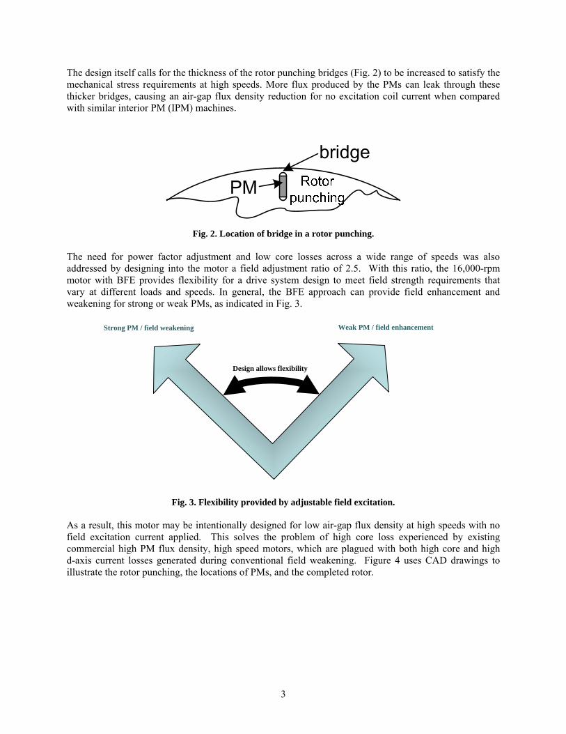
The design itself calls for the thickness of the rotor punching bridges (Fig. 2) to be increased to satisfy the mechanical stress requirements at high speeds. More flux produced by the PMs can leak through these thicker bridges, causing an air-gap flux density reduction for no excitation coil current when compared with similar interior PM (IPM) machines.

Fig. 2. Location of bridge in a rotor punching.

The need for power factor adjustment and low core losses across a wide range of speeds was also addressed by designing into the motor a field adjustment ratio of 2.5. With this ratio, the 16,000-rpm motor with BFE provides flexibility for a drive system design to meet field strength requirements that vary at different loads and speeds. In general, the BFE approach can provide field enhancement and weakening for strong or weak PMs, as indicated in Fig. 3.

Fig. 3. Flexibility provided by adjustable field excitation. As a result, this motor may be intentionally designed for low air-gap flux density at high speeds with no field excitation current applied. This solves the problem of high core loss experienced by existing commercial high PM flux density, high speed motors, which are plagued with both high core and high d-axis current losses generated during conventional field weakening. Figure 4 uses CAD drawings to illustrate the rotor punching, the locations of PMs, and the completed rotor.

Strong PM / field weakening Weak PM / field enhancement

Design allows flexibility

4

Fig. 4. Rotor CAD drawing of ORNL’s 16,000-rpm motor.

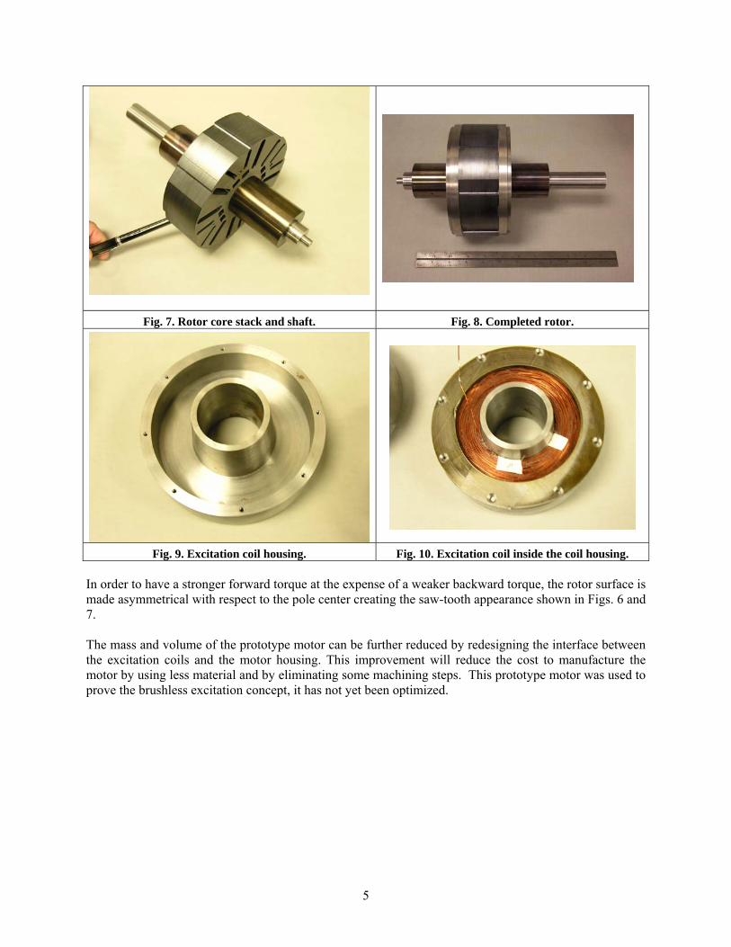
Figures 5 through 10 are photographs of actual hardware showing the wound stator core, a stack of rotor punchings, a rotor core stack and shaft, a completed rotor, excitation coil housing, and an excitation coil inside the coil housing of the prototype motor.

Fig. 5. Wound stator core. Fig. 6. Rotor punching.

Rotor Core Punching Stack

PM Arrangement

Completed Rotor

5

Fig. 7. Rotor core stack and shaft. Fig. 8. Completed rotor.

Fig. 9. Excitation coil housing. Fig. 10. Excitation coil inside the coil housing. In order to have a stronger forward torque at the expense of a weaker backward torque, the rotor surface is made asymmetrical with respect to the pole center creating the saw-tooth appearance shown in Figs. 6 and 7. The mass and volume of the prototype motor can be further reduced by redesigning the interface between the excitation coils and the motor housing. This improvement will reduce the cost to manufacture the motor by using less material and by eliminating some machining steps. This prototype motor was used to prove the brushless excitation concept, it has not yet been optimized.

6

AIR GAP FLUX, INDUCTANCE, PERFORMANCE PARAMETER COMPUTATIONS, AND COMPARISONS OF SIMULATION WITH TEST RESULTS

Figure 11 shows the calculated air-gap flux density distributions at various excitation levels. The field excitation, Iexc, is the product of current flowing through the excitation coil and the 865 turns in the field coil. The excitation current, Iexc, can be calculated by dividing the ampere-turns (AT) by the number of turns in the field coil. The air-gap flux density is adjusted by varying the field excitation current. When high torque is required, the air-gap flux density is enhanced by increasing Iexc. When low torque and high efficiency are required, Iexc is reduced to zero.

-2.5

-2

-1.5

-1

-0.5

0

0.5

1

1.5

2

Rotor Angle (Electrical degree)

Flux

Den

sity

[ T

Iexc=-1000 AT, Bg1=0.03816 TIexc=0 AT, Bg1=0.2437 TIexc=1000 AT, Bg1=0.5598 TIexc=2000 AT, Bg1=0.8688 TIexc=3000 AT, Bg1=1.0313TIexc=4000 AT, Bg1=1.0588 TIexc=5000 AT, Bg1=1.0615 T

Fig. 11. Air-gap flux density distributions for various field excitations.

Figure 12 shows the expected 16,000-rpm motor torque versus load angle at the maximum stator winding current amplitude, Imax = 200A, for different field excitations. Greater excitation produces stronger motor torque.

7

-50

0

50

100

150

200

90 105 120 135 150 165 180

Load Angle [Electrical degree]

Torq

ue [N

.m]

Iexc=5000 AT, Tmax=158.27 NmIexc=4000 AT, Tmax=146.49 NmIexc=3000 AT, Tmax=130.09 NmIexc=2000 AT, Tmax=107.13 NmIexc=1000 AT, Tmax=82.78 NmIexc=0 AT, Tmax=68.60 Nm

Fig. 12. Expected motor torque vs. load angle at Imax = 200A for different field excitations.

Figure 13 is the simulation results of an expected phase back-emf voltage waveform for 5000AT field excitation at 5000 rpm. This waveform is calculated from the time derivative of flux linkage at one of the phase conductors. The corresponding fundamental component is also shown.

-500

-400

-300

-200

-100

0

100

200

300

400

500

0 3 6 9 12

time [msec]

Bac

k EM

F [V

]

Expected wave formFundamental

Fig. 13. Simulation results of a voltage phase back-emf at Iexc = 5000 AT and 5000 rpm.

8

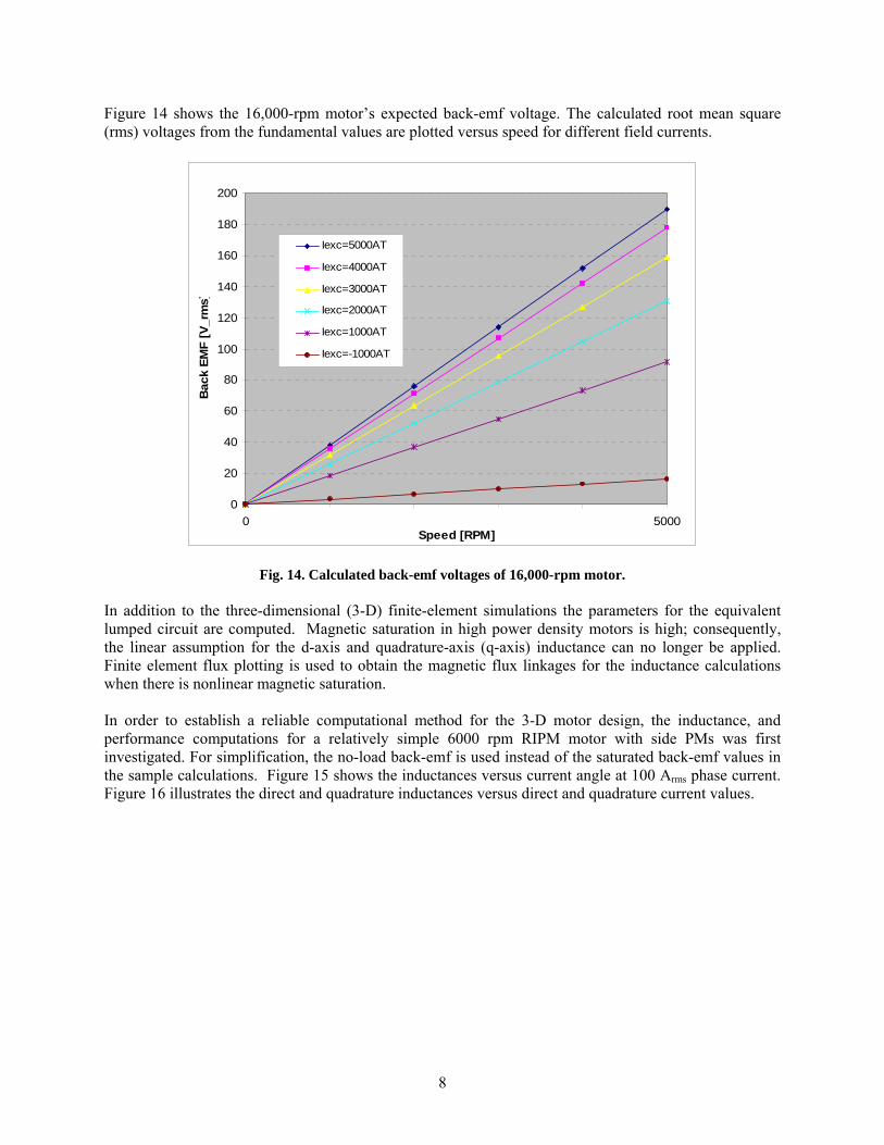
Figure 14 shows the 16,000-rpm motor’s expected back-emf voltage. The calculated root mean square (rms) voltages from the fundamental values are plotted versus speed for different field currents.

0

20

40

60

80

100

120

140

160

180

200

0 5000Speed [RPM]

Bac

k EM

F [V

_rm

s]

Iexc=5000AT

Iexc=4000AT

Iexc=3000AT

Iexc=2000AT

Iexc=1000AT

Iexc=-1000AT

Fig. 14. Calculated back-emf voltages of 16,000-rpm motor.

In addition to the three-dimensional (3-D) finite-element simulations the parameters for the equivalent lumped circuit are computed. Magnetic saturation in high power density motors is high; consequently, the linear assumption for the d-axis and quadrature-axis (q-axis) inductance can no longer be applied. Finite element flux plotting is used to obtain the magnetic flux linkages for the inductance calculations when there is nonlinear magnetic saturation. In order to establish a reliable computational method for the 3-D motor design, the inductance, and performance computations for a relatively simple 6000 rpm RIPM motor with side PMs was first investigated. For simplification, the no-load back-emf is used instead of the saturated back-emf values in the sample calculations. Figure 15 shows the inductances versus current angle at 100 Arms phase current. Figure 16 illustrates the direct and quadrature inductances versus direct and quadrature current values.

9

0

0.5

1

1.5

2

2.5

3

3.5

90 120 150 180

Current Angle* [deg]

Ld, L

q [m

H]

Ld with magnetic saturation

Lq with magnetic saturation

Ld without magnetic saturation

Lq without magnetic saturation

* Id = Iph,max cosβ and Iq = Iph,max sinβ, where β is the current angle. When the current angle is 90°,

Id = 0 and Iq = Iph,max. When the current angle is 180°, Id = -Iph,max and Iq = 0.

Fig. 15. Inductances vs. current angle at 100 Arms phase current.

Inductance vs. Current value

0

0.5

1

1.5

2

2.5

3

0 30 60 90 120 150Id, Iq [A]

Ld, L

q [m

H]

Ld @ Iq = 0A

Lq @ Id = 0A

Fig. 16. Inductances vs. current values.

10

The performance of the simple 6000 rpm RIPM motor with side PMs was calculated with the inductance values shown in Figs. 15 and 16 at 3498 rpm and an input voltage of 233.22 Vrms. The comparison between the simulated and test results are listed in Table 2. It should be pointed out that the power factor for the simulation is based on the fundamental values and the test power factor is the total power factor, which includes all the harmonics. The simulation may be improved by using the saturated back-emf values instead of the no-load back-emf values.

Table 2. Comparison between simulated results and test results for the simple 6000 rpm RIPM motor at 3500 rpm and 233 Vrms.

Unit Simulation

Results Test Results Simulation/Test

Torque Newton meter (Nm) 127.24 109.38 1.16

Speed rpm 3498 3498 1.00 Pmotor kW 46.61 40.07 1.16

Back-emf* (rms) V 203.12 213.78 0.95 Input Voltage (rms) V 233.22 233.22 1.00 Input Current (rms) A 87.5 102.22 0.86

Power Factor - 0.85 0.64 1.33 Pinput kW 52.04 45.44 1.15

Efficiency % 89.56 88.18 1.02 * Back-emf voltage is from no-load simulation and test.

Figure 17 shows the simulated vector diagram of the simple 6000-rpm RIPM motor at 3500 rpm and 233 Vrms.

Fig. 17. Simulated phasor diagram of the simple 6000 rpm RIPM motor with side PMs at 3500 rpm and 233 Vrms.

11

The simulation of the simple 6000 rpm RIPM motor with side PMs was again calculated with the inductance values shown in Figs. 15 and 16 at 3498 rpm, but this time at an input current of 102.22 Arms. The comparison between the simulated and test results are listed in Table 3. Once again the power factor for the simulation is based on the fundamental values and the test power factor is the total power factor that includes all the voltage and current harmonics. In the future, the simulation may be improved by using the saturated back-emf values instead of the no-load back-emf values. Table 3. Comparison between simulated results and test results of the

simple 6000 rpm RIPM motor at 3500 rpm and 102 Arms

Unit Simulation Results Test Results Simulation/Test

Torque Nm 141.56 109.38 1.29 Speed rpm 3498 3498 1.00 Pmotor kW 51.85 40.07 1.29

Back-emf* V 203.12 213.78 0.95 Input Voltage

(rms) V 251.06 233.22 1.08

Input Current (rms) A 102.22 102.22 1.00 Power Factor - 0.79 0.64 1.23

Pinput kW 60.82 45.44 1.34 Efficiency % 85.28 88.18 0.97

• Back-emf voltage is from no-load simulation and test.

Figure 18 shows the simulated phasor diagram of the simple 6000 rpm RIPM motor with side PMs at 3500 rpm and 100 Arms.

Fig. 18. Simulated phasor diagram of the simple 6000 rpm RIPM motor with side PMs at 3500 rpm and 100 Arms.

12

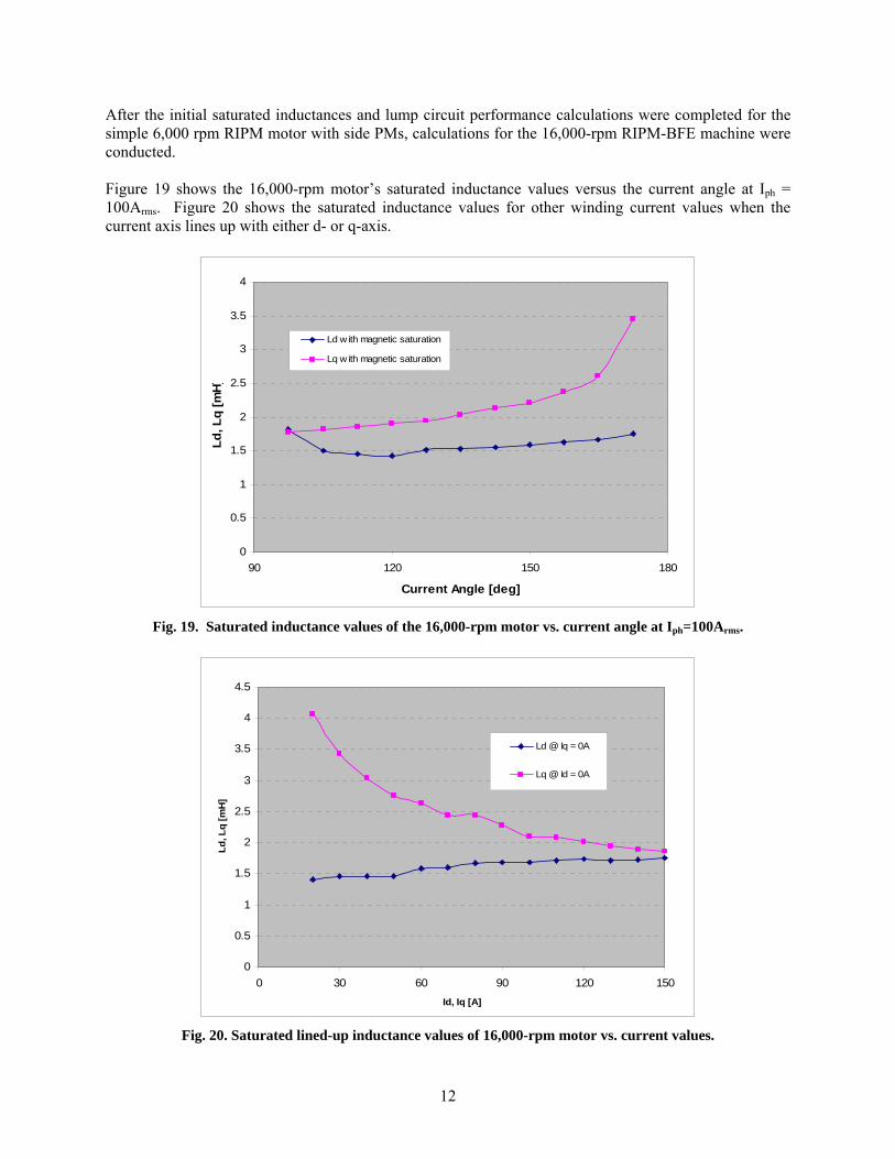
After the initial saturated inductances and lump circuit performance calculations were completed for the simple 6,000 rpm RIPM motor with side PMs, calculations for the 16,000-rpm RIPM-BFE machine were conducted. Figure 19 shows the 16,000-rpm motor’s saturated inductance values versus the current angle at Iph = 100Arms. Figure 20 shows the saturated inductance values for other winding current values when the current axis lines up with either d- or q-axis.

0

0.5

1

1.5

2

2.5

3

3.5

4

90 120 150 180

Current Angle [deg]

Ld, L

q [m

H]

Ld w ith magnetic saturation

Lq w ith magnetic saturation

Fig. 19. Saturated inductance values of the 16,000-rpm motor vs. current angle at Iph=100Arms.

0

0.5

1

1.5

2

2.5

3

3.5

4

4.5

0 30 60 90 120 150Id, Iq [A]

Ld, L

q [m

H]

Ld @ Iq = 0A

Lq @ Id = 0A

Fig. 20. Saturated lined-up inductance values of 16,000-rpm motor vs. current values.

13

The performance of the 16,000-rpm RIPM-BFE motor with 5A in the BFE coil was calculated with the saturated inductances shown in Figs. 21 and 22 and an input voltage of 270.01 Vrms. The comparison between the simulated and test results appear in Table 4 followed by a phasor diagram. Correspondingly, the performance of the same motor was calculated for an input current of 100 Arms with the comparison in Table 5 followed by a phasor diagram. Use of the saturated inductances appears to have improved the agreement.

Fig. 21. Simulated phasor diagram of 16,000-rpm IPM synchronous motor (SM) at 3,300 rpm, 5 A excitation, and 270 Vrms.

Fig. 22. Simulated phasor diagram of 16,000-rpm IPM SM at 3,300 rpm, 5A excitation, and 100 Arms.

14

Table 4. Comparison between simulated results and test results of 16,000-rpm motor

at given speed and input voltage

Unit Simulation Results Test Results Simulation/Test

Torque Nm 115.08 105.02 1.10 Speed rpm 3300 3300 1.00 Pmotor kW 39.77 36.29 1.10

Back-emf* V 121.32 129.39 0.94 Input Voltage (rms) V 270.01 270.01 1.00 Input Current (rms) A 112.10 102.39 1.09

Power Factor - 0.50 0.47 1.06 Pinput kW 45.40 38.89 1.17

Efficiency % 87.60 93.33 0.94 • Back-emf voltage is from no-load simulation and test.

Table 5. Comparison between simulated results and test results of 16,000-rpm motor at given speed and input current

Unit Simulation

Results Test Results Simulation/Test

Torque Nm 102.24 105.02 0.97 Speed rpm 3300 3300 1.00 Pmotor kW 35.33 36.29 0.97

Back-emf*(rms) V 121.32 129.39 0.94 Input Voltage (rms) V 248.22 270.01 0.92 Input Current (rms) A 102.39 102.39 1.00

Power Factor - 0.53 0.47 1.13 Pinput kW 40.41 38.89 1.04

Efficiency % 87.43 93.33 0.94 • Back-emf voltage is from no-load simulation and test.

15

MECHANICAL STRESS COMPUTATIONS

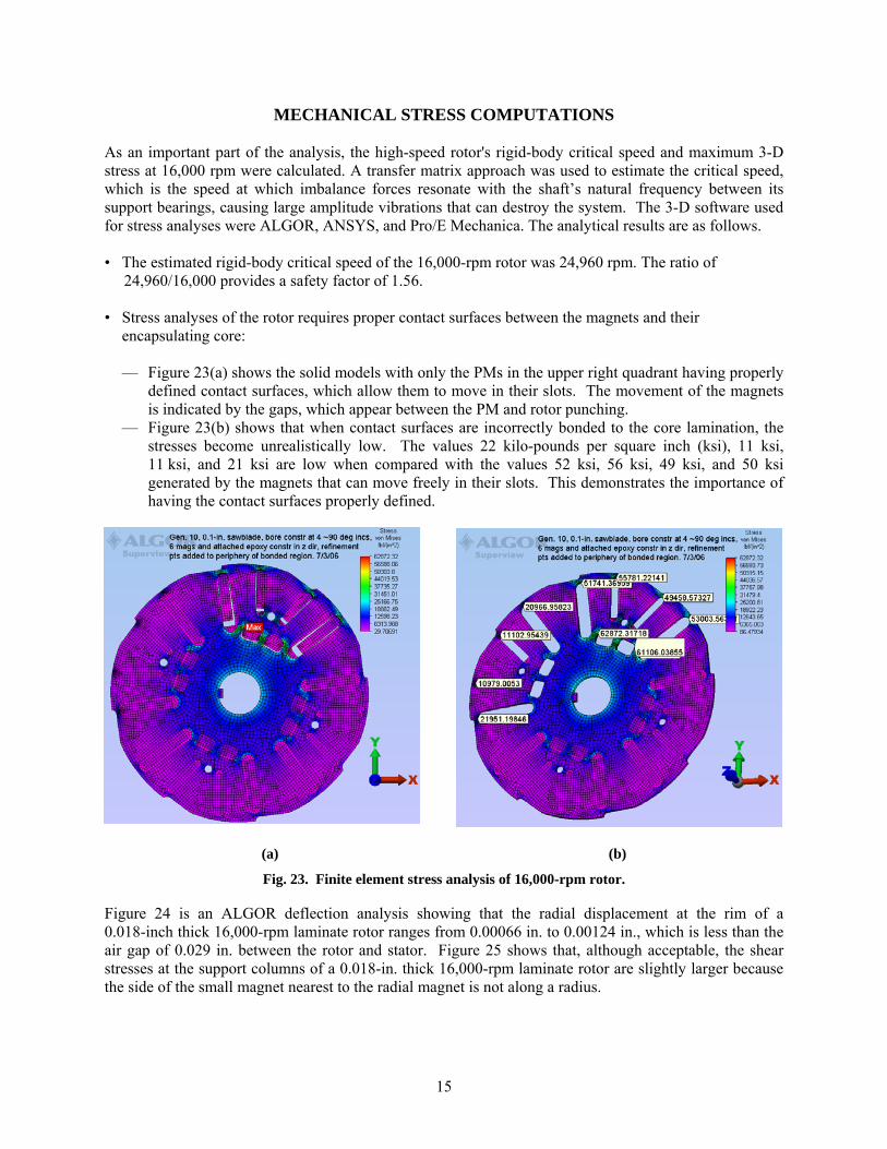
As an important part of the analysis, the high-speed rotor's rigid-body critical speed and maximum 3-D stress at 16,000 rpm were calculated. A transfer matrix approach was used to estimate the critical speed, which is the speed at which imbalance forces resonate with the shaft’s natural frequency between its support bearings, causing large amplitude vibrations that can destroy the system. The 3-D software used for stress analyses were ALGOR, ANSYS, and Pro/E Mechanica. The analytical results are as follows.

• The estimated rigid-body critical speed of the 16,000-rpm rotor was 24,960 rpm. The ratio of

24,960/16,000 provides a safety factor of 1.56.

• Stress analyses of the rotor requires proper contact surfaces between the magnets and their encapsulating core: — Figure 23(a) shows the solid models with only the PMs in the upper right quadrant having properly

defined contact surfaces, which allow them to move in their slots. The movement of the magnets is indicated by the gaps, which appear between the PM and rotor punching.

— Figure 23(b) shows that when contact surfaces are incorrectly bonded to the core lamination, the stresses become unrealistically low. The values 22 kilo-pounds per square inch (ksi), 11 ksi, 11 ksi, and 21 ksi are low when compared with the values 52 ksi, 56 ksi, 49 ksi, and 50 ksi generated by the magnets that can move freely in their slots. This demonstrates the importance of having the contact surfaces properly defined.

(a) (b)

Fig. 23. Finite element stress analysis of 16,000-rpm rotor.

Figure 24 is an ALGOR deflection analysis showing that the radial displacement at the rim of a 0.018-inch thick 16,000-rpm laminate rotor ranges from 0.00066 in. to 0.00124 in., which is less than the air gap of 0.029 in. between the rotor and stator. Figure 25 shows that, although acceptable, the shear stresses at the support columns of a 0.018-in. thick 16,000-rpm laminate rotor are slightly larger because the side of the small magnet nearest to the radial magnet is not along a radius.

16

Fig. 24. Radial displacement of the 16,000-rpm rotor.

Fig. 25. Shear stresses at the support columns of a 0.018-in.

thick 16,000-rpm laminate rotor.

17

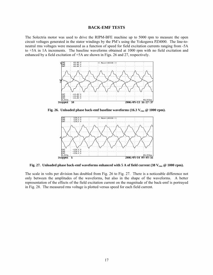
BACK-EMF TESTS The Solectria motor was used to drive the RIPM-BFE machine up to 5000 rpm to measure the open circuit voltages generated in the stator windings by the PM’s using the Yokogawa PZ4000. The line-to-neutral rms voltages were measured as a function of speed for field excitation currents ranging from -5A to +5A in 1A increments. The baseline waveforms obtained at 1000 rpm with no field excitation and enhanced by a field excitation of +5A are shown in Figs. 26 and 27, respectively.

Fig. 26. Unloaded phase back-emf baseline waveforms (16.3 Vrms @ 1000 rpm).

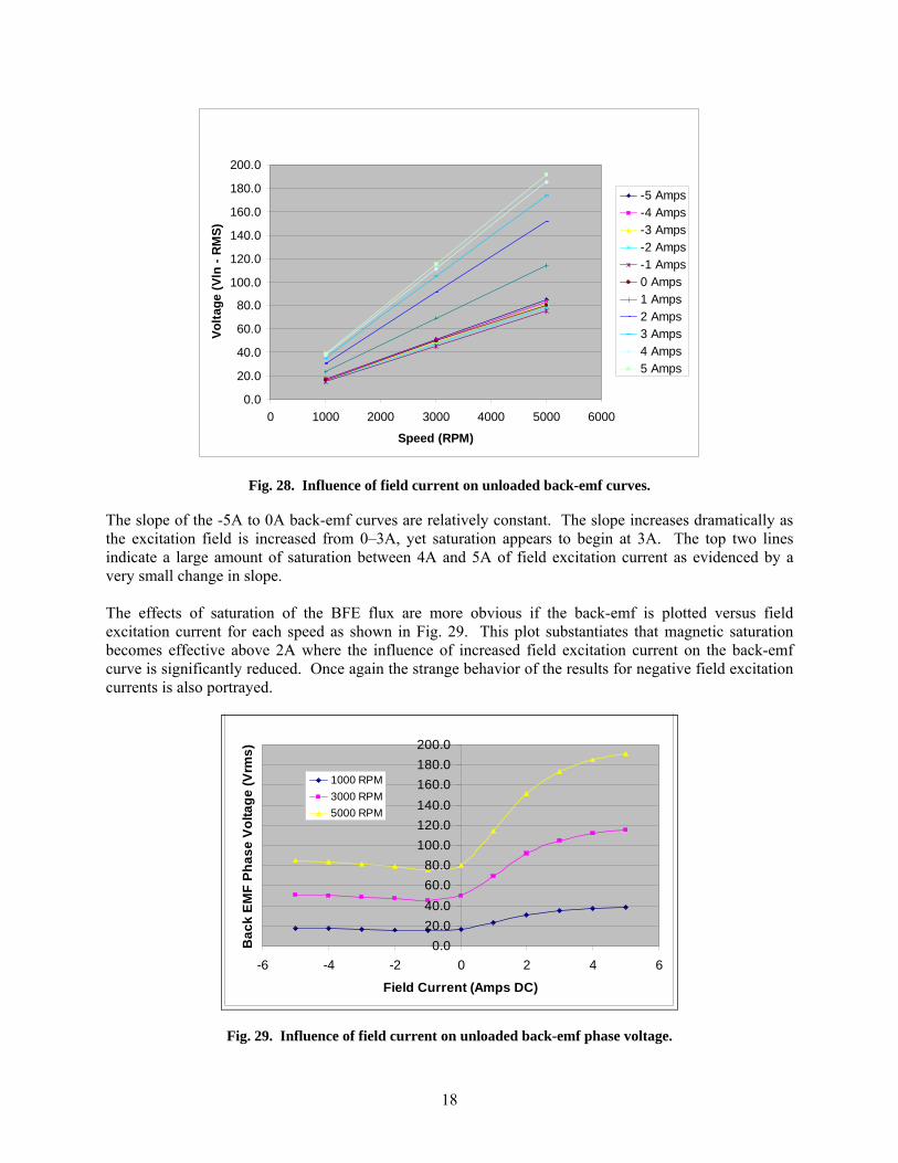
Fig. 27. Unloaded phase back-emf waveforms enhanced with 5 A of field current (38 Vrms @ 1000 rpm). The scale in volts per division has doubled from Fig. 26 to Fig. 27. There is a noticeable difference not only between the amplitudes of the waveforms, but also in the shape of the waveforms. A better representation of the effects of the field excitation current on the magnitude of the back-emf is portrayed in Fig. 28. The measured rms voltage is plotted versus speed for each field current.

18

Back-EMF Voltage vs Speed (Vln - RMS)

0.0

20.0

40.0

60.0

80.0

100.0

120.0

140.0

160.0

180.0

200.0

0 1000 2000 3000 4000 5000 6000

Speed (RPM)

Volta

ge (V

ln -

RM

S)-5 Amps-4 Amps-3 Amps-2 Amps-1 Amps0 Amps1 Amps2 Amps3 Amps4 Amps5 Amps

Fig. 28. Influence of field current on unloaded back-emf curves.

The slope of the -5A to 0A back-emf curves are relatively constant. The slope increases dramatically as the excitation field is increased from 0–3A, yet saturation appears to begin at 3A. The top two lines indicate a large amount of saturation between 4A and 5A of field excitation current as evidenced by a very small change in slope. The effects of saturation of the BFE flux are more obvious if the back-emf is plotted versus field excitation current for each speed as shown in Fig. 29. This plot substantiates that magnetic saturation becomes effective above 2A where the influence of increased field excitation current on the back-emf curve is significantly reduced. Once again the strange behavior of the results for negative field excitation currents is also portrayed.

0.020.040.060.080.0

100.0120.0140.0160.0180.0200.0

-6 -4 -2 0 2 4 6

Field Current (Amps DC)

Bac

k EM

F Ph

ase

Volta

ge (V

rms)

1000 RPM3000 RPM5000 RPM

Fig. 29. Influence of field current on unloaded back-emf phase voltage.

19

From the measured back-emf per phase versus the field current shown in Fig. 29, the test field adjustment ratio, which is the phase back-emf at a given field excitation current divided by the back-emf at 0A field excitation current, can be obtained. These test field adjustment ratios are listed in Table 6. The ratio indicates how the field excitation current can change the phase back-emf.

Table 6. Test field adjustment ratios

Speed [rpm]

Field current[A]

Phase emf[Vrms] Field adj. ratio

0 80 1.0 2 152 1.9

5000

5 191 2.4 0 50 1.0 2 92 1.8

3000

5 116 2.3 0 18 1.0 2 30 1.7

1000

5 39 2.2

20

CORE/FRICTION LOSS TESTS These tests were conducted by using the Solectria motor to spin the RIPM-BFE motor while measuring the load created at the RIPM-BFE shaft due to friction and core effects with the motor leads disconnected and floating. Similar to the back-emf tests, these tests were conducted as the field current was varied from -5A to +5A in 1A increments. The results are shown in Fig. 30 with the measured torque plotted versus speed for the various field currents. Torque saturation with respect to speed appears for negative excitation field currents at high speeds, as indicated by leveling of the dotted lines in Fig.30. In Fig. 31, the torque data was converted to power, which is the product of torque and speed, and plotted versus speed. These plots show that the losses increase whether the excitation field enhances or weakens the field of the PM, but are much greater for the enhanced excitation field.

No-Load Driven Torque Vs Speed for each Field Current

0.2

0.3

0.4

0.5

0.6

0.7

0.8

0.9

1

1.1

1.2

500 1500 2500 3500 4500 5500

Speed (RPM)

Torq

ue (N

m)

-5A

-4A

-3A

-2A

-1A

0A1A

2A

3A

4A

5A

Fig. 30. Influence of field excitation current on torque needed to overcome unloaded core and friction losses.

21

Core and Friction losses Vs Speed for each Field Current

0.2

100.2

200.2

300.2

400.2

500.2

600.2

700.2

500 1500 2500 3500 4500 5500

Speed (RPM)

Pow

er (W

)-5A

-4A

-3A

-2A

-1A

0A

1A

2A

3A

4A

5A

Fig. 31. Influence of field excitation current on unloaded core and friction losses. An important feature of RIPM-BFE technology is revealed by plotting power loss versus field current for each speed, as shown in Fig. 32. Notice the high power loss for the 5A and 5000 rpm operation point. For other motors with similar torque and power ratings, the power loss would be constant regardless of the torque requirement. For our example, the loss is 600 W; however, for the RIPM BFE if the maximum flux is not needed, the field current, and therefore the air gap flux, can be lowered to dramatically reduce the losses to 200 W for no excitation field current. This is a key advantage of the RIPM-BFE machine, and its impact on efficiency will be most evident in the low torque region of the efficiency map.

22

Core and Friction Loss vs Field Current For Each Speed

0.0

100.0

200.0

300.0

400.0

500.0

600.0

-6 -4 -2 0 2 4 6

Field Current (Amps DC)

Pow

er (W

)

1000 rpm

3000 rpm

5000 rpm

Fig. 32. Influence of field current on core losses.

23

LOCKED ROTOR TESTS During the locked rotor tests, the rotor was fixed at selected angular positions as positive dc current was fed to phase ‘a’ and returned through phases ‘b’ and ‘c’ connected in parallel. The results for a stator current of 50A and various field currents are shown in Fig. 33. Contrary to the waveform shape of typical PM synchronous motors (PMSMs), these torque waveforms are not symmetrical about the horizontal axis. For example, for no field excitation current the magnitude of the peak positive torque, 16 Nm, does not equal the magnitude of the peak negative torque, -24 Nm. This feature was purposely designed into the RIPM-BFE motor to produce more torque while spinning in one direction than in the opposite direction; consequently, it was necessary to spin the motor in the appropriate direction during testing.

Locked Rotor Torque - 50 Amps DC

-50.00

-40.00

-30.00

-20.00

-10.00

0.00

10.00

20.00

30.00

40.00

50.00

0.00 100.00 200.00 300.00 400.00

Position (Electrical Degrees)

Torq

ue (N

m)

5A3A0A-3A

Fig. 33. Locked rotor torque for the RIPM-BFE motor. As expected, the peak torque is obtained while using the highest field excitation current of 5A. The torque measurements for all stator currents with 5A field current are shown in Fig. 34. Only the peak regions were measured for stator currents other than 50A to reduce test time and to avoid the temperature rise that accompanies higher stator currents. The graph shows that the peak torque capability of the motor is about -155 Nm. The effect of flux saturation due to the stator current is more easily visualized when the peak torques are plotted versus stator current, as shown in Fig. 35. Saturation due to stator current begins to have a significant impact on the torque production near about 150A dc.

24

Locked Rotor Torque With 5A Field Current

-200.00

-150.00

-100.00

-50.00

0.00

50.00

100.00

150.00

0.00 50.00 100.00 150.00 200.00 250.00 300.00 350.00 400.00

Position (Electrical Degrees)

Torq

ue (N

m)

50A100A150A200A250A300A350A

Fig. 34. Locked rotor torque with 5A field excitation current.

Peak Torque Per Stator Current

0

20

40

60

80

100

120

140

160

180

0 50 100 150 200 250 300 350 400

Stator Current (Amps DC)

Torq

ue (N

m)

-5A

-3A

0A

3A

5A

Fig. 35. Impact of flux saturation on peak torque.

25

PERFORMANCE/EFFICIENCY TESTS The motor was driven at various speed-torque operation points in order to collect a vast amount of data, which includes temperatures, powers, currents, voltages, and efficiencies. The temperatures remained well within the stator winding limitations, which is 220°C (class R). For most of the data points, all temperatures remained below 100°C; yet for high current conditions, temperatures reached about 135°C. Note however that tap water at about 15°C was fed into the water/oil heat exchanger, which is a significant advantage over much warmer coolant. Use of a refrigerant will also provide heat dissipation capabilities closer to that of the cold tap water. Performance/efficiency tests were conducted with field currents of 0A and 5A, and the winding to ground failure prevented completion of the 5A and the entire 3A performance mapping. These evaluations will be further discussed in this report to indicate the unexpected damage on the rewound motor and to project the results if the motor was not damaged. The motor efficiency is the quotient of the mechanical power delivered to the dynamometer and the ac power supplied to the motor. The efficiency contour map obtained while using no field excitation current is shown in Fig. 36. A maximum torque of 85 Nm was reached at low speeds and a power level of about 23 kW was reached at 4900 rpm. The highest efficiencies are shown for relatively low torques and speeds above 1200 rpm.

Fig. 36. Efficiency contours for the RIPM-BFE motor with no field excitation current.

Because the copper loss of the field coil depends on the available field coil copper space and can be reduced by increasing the copper space, the efficiency contours shown in Fig. 37 exclude resistive power loss of the BFE field coil for the 5A tests. These losses of the prototype motor were about 400 W (80 V and 5 A). When the BFE losses are incorporated, the efficiencies are slightly lower, as shown in Fig. 38. At low torques where the power levels are low, the 400 W loss of the field coil has more effect upon efficiency than it does at high power levels. The Fig. 36 efficiency map with no excitation was rescaled in Fig. 39 for direct comparison with the Fig. 37 efficiency map measured when the field excitation was 5A. Examination of the regions above

26

90% efficiency in Fig. 39 shows that this region extends down to 1000 rpm in the low-torque region for no field excitation current. Figure 40 is a combination of the information from Figs. 38 and 39 from which the maximum of the two efficiencies at each torque/speed point was plotted. This is a rough representation from only two field excitation cases to show how the field current may be adjusted to improve the efficiency contour map. It will show later when six field excitation currents between 0 and 5 A are used, these contours become smoother due to more interpolation. Additionally, the advantage of flux weakening via the BFE coils will be much more noticeable at high speeds.

Fig. 37. Efficiency contours with 5A field excitation current excluding resistive losses of the BFE field coil.

Fig. 38. Efficiency contours including 5A resistive losses of the BFE field coil.

27

Fig. 39. Baseline (no field excitation current) efficiency contour map scaled for comparison

with the contour map measured using 5A field excitation current.

Fig. 40. Greater efficiency plot from efficiency contour maps for 0A and 5A field excitation currents showing

how field excitation may be used to improve efficiency contours. To provide a good comparison with the baseline (Prius) motor, a high speed gear could be included in the mapping to convert from a maximum speed of 16,000 rpm to 6,000 rpm. A gear ratio of about 2.6 will suffice, which also changes the maximum torque from 155 Nm to about 400 Nm. The resulting

28

efficiency map is shown in Fig. 41 for comparison with the Prius efficiency map in Fig. 42. Although a large portion of the RIPM-BFE map is missing, a comparison of the low speed efficiencies is informative. The efficiency of the RIPM BFE in the low speed region is significantly better. It is also apparent that the 93% and 94 % contours will be much larger.

Fig. 41. RIPM BFE efficiency map with high speed gear ratio of 2.6.

Fig. 42. Baseline (Prius motor) efficiency map.

29

Part of the advantage of the ORNL RIPM-BFE motor over the baseline motor, after considering the losses from the gears and from the field excitation, is due to the high speed gear reduction. However, the RIPM BFE still has the advantage of using an optimal field current, and by reducing the air gap flux when it is not needed, the efficiency may be increased at low torques both at partial loads and at high speeds. This is confirmed by comparing Figs. 41 and 42 for the low speed region. The high speed projected tests will show later in this report for the similar efficiency advantages. Comparison of the test efficiency maps between the ORNL motor (Fig. 41) and the baseline (Prius) motor (Fig. 42) shows that the 94% efficiency contour of the ORNL motor starts at 1400 rpm, the baseline motor starts at 2200 rpm and covers a very small region. The available performance test data up to 3700 rpm (or 3700/2.6 = 1423 equivalent rpm after gears) confirm that the ORNL motor has higher efficiency than the baseline motor.

30

REWOUND MOTOR TESTS During the first series of tests on the 16,000-rpm RIPM BFE, a failure occurred in the stator windings in which a short was created to ground. The failure was possibly due to localized lamination vibration that eventually wore down the slot insulation between the stator windings and stator laminations in the corner of a slot opening. Fortunately, most of the planned low-speed tests were conducted before the failure and enough data was collected to draw sufficient conclusions. The stator was sent to the original manufacturer to be rewound, wherein the inner diameter of the stator laminations was increased slightly to enable removal of the defective windings, as shown in Fig. 43. Therefore, the air gap between the rotor and stator was increased and the flux generated by the PMs, stator windings, and field windings is now further inhibited. A second series of tests were conducted with the rewound stator installed into the same housing used in the first series of tests. A spline was added to the original rotor to provide an interface with the high-speed side of the newly installed speed reduction gearbox. A comparison of efficiencies obtained from the first and second series of tests yields significant discrepancies.

Fig. 43. Stator before (left) and after (right) rewinding.

31

BACK-EMF RESULTS

Back-emf tests were conducted with various field excitation currents, as shown in Fig. 44. Test results from both stators are shown for field currents of 0A and 5A, wherein the induced back-emf voltage of the second stator is about 4% lower than that of the first stator, which indicates that the flux through the stator windings is about 4% lower as the back-emf voltage is directly proportional to flux and speed. Since the 0A back-emf results indicate a similar decrease of voltage, the field windings are not suspected to be defective.

Back-EMF vs Speed

0

20

40

60

80

100

120

140

160

180

200

0 1000 2000 3000 4000 5000 6000

Speed (RPM)

Line

-Neu

tral

Vol

tage

(Vrm

s)

Stator 1 0A

Stator 1 5AStator 2 0AStator 2 5A

Fig. 44. Back-emf voltage vs. speed for both stators.

32

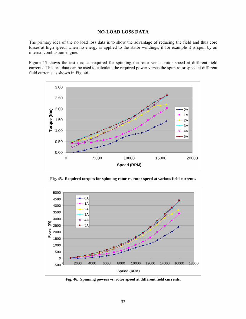
NO-LOAD LOSS DATA The primary idea of the no load loss data is to show the advantage of reducing the field and thus core losses at high speed, when no energy is applied to the stator windings, if for example it is spun by an internal combustion engine. Figure 45 shows the test torques required for spinning the rotor versus rotor speed at different field currents. This test data can be used to calculate the required power versus the spun rotor speed at different field currents as shown in Fig. 46.

0.00

0.50

1.00

1.50

2.00

2.50

3.00

0 5000 10000 15000 20000

Speed (RPM)

Torq

ue (N

m) 0A

1A2A3A4A5A

Fig. 45. Required torques for spinning rotor vs. rotor speed at various field currents.

-500

0

500

1000

1500

2000

2500

3000

3500

4000

4500

5000

0 2000 4000 6000 8000 10000 12000 14000 16000 18000

Speed (RPM)

Pow

er (W

)

0A1A2A3A4A5A

Fig. 46. Spinning powers vs. rotor speed at different field currents.

33

Figure 47 shows that the data can be rearranged to plot the spinning losses versus field current for various rotor speeds. The spinning loss can be greater than double when the field is strong. Figure 47 confirms the advantage of the field control capability of the RIPM-BFE motor; the loss is significantly reduced when spinning at high speed with zero field current.

Fig. 47. Spinning losses vs. field current for various rotor speeds.

34

EFFICIENCY MAPPING Efficiency tests were conducted using the same approach that was taken in the first series of tests. Optimal motor control was insured by observing efficiency feedback as control conditions were varied throughout the entire operation range. Data points for each efficiency map were taken from 1,000 rpm to 16,000 in 1,000 rpm increments and from 0 Nm increasing in 10 Nm increments to a final high torque value at each speed. A total of six efficiency maps were generated for corresponding dc field currents of 0A, 1A, 2A, 3A, 4A, and 5A which are shown in the Appendix. For instance, the 16,000-rpm RIPM BFE efficiency contours with 5A field without field losses are shown in Fig. 48.

Fig. 48. 16,000-rpm RIPM BFE efficiency contours with 5 A field without field losses.

A consistent scale for torque and speed was used to clarify the differences between the efficiency maps. The optimal efficiency of all field currents for each torque and speed (without field winding losses considered) was selected to produce the optimized efficiency map shown in Fig. 49. The corresponding optimal field currents were mapped for the entire torque-speed range, as shown in Fig. 50. For a large portion of the speed operation range, the most optimal field current to use while producing high torque or high power is 5A. A peak efficiency of 93% is obtained at 5000 rpm and 50 Nm while using a field current of 3A. Note that a speed limit of about 10,000 rpm was imposed for field currents below 5A to prevent failures associated with over-voltage, particularly on the dc-link which will reach over 1,200 V when the sinusoidal back-emf is rectified. During these tests, it is common to shut down and restart the motor when instability is reached, which is inevitable since optimal operation at high speeds is barely within the voltage limit range. In application, the controller would be programmed to operate within these limits and in the rare event of instability, it would also turn off power to the field winding to reduce the induced back-emf voltage prior to releasing the power applied to the stator windings.

35

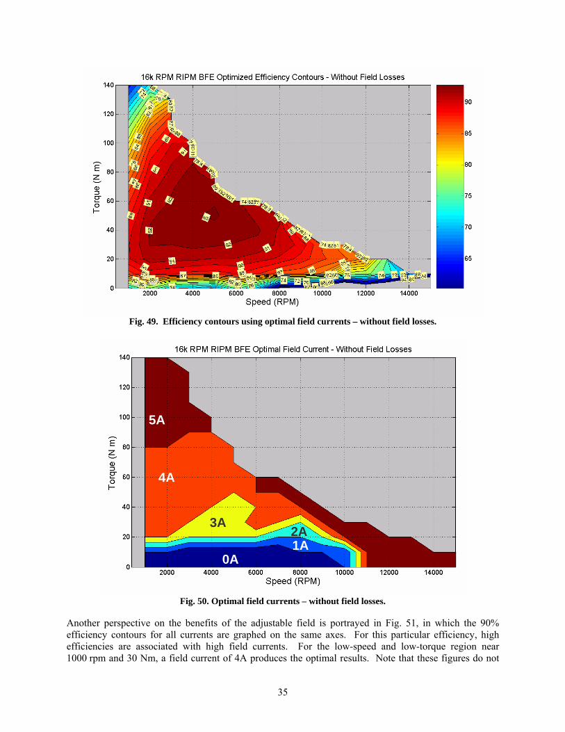
Fig. 49. Efficiency contours using optimal field currents – without field losses.

Fig. 50. Optimal field currents – without field losses.

Another perspective on the benefits of the adjustable field is portrayed in Fig. 51, in which the 90% efficiency contours for all currents are graphed on the same axes. For this particular efficiency, high efficiencies are associated with high field currents. For the low-speed and low-torque region near 1000 rpm and 30 Nm, a field current of 4A produces the optimal results. Note that these figures do not

5A

4A

0A 1A

3A 2A

36

account for field losses and the effects of variable field currents will be more substantial when field losses are considered. Nonetheless, these figures still hold importance as the effects from the variable field current are observed, while showing the potential of the system if a more efficient means of field excitation is developed.

Fig. 51. Efficiency contours for 90% without field losses for all field currents.

The power associated with field excitation will impact the efficiency contours significantly, particularly for high field currents and low mechanical power levels. There are two excitation coils with resistances of about 8 ohms each. The coils were connected in series, giving a power requirement of Pexc ≈ Iexc

2 16, and a voltage requirement of Vexc ≈ Iexc 16. So for 5A operation, the power and voltage requirements are 400 W and 80 VDC, respectively. Therefore, if the system is operating at 10 kW, about 4% of the power is devoted to the field excitation. Incorporating this power requirement with the 5A efficiency data produces the efficiency map shown in Fig. 52. A comparison of the 5A efficiency maps in Figs. 48 and 52, which neglect and consider field losses respectively, provides deeper insight into the effects of the field losses, particularly for low-torque regions. An even more interesting comparison is observed when comparing 0A and 5A efficiency maps in the Appendix. The low-speed, low-torque region of the 0A map reveals much higher efficiencies than that of the 5A efficiency map. As the field current increases, this high efficiency region expands and moves to regions of higher torques and higher speeds. Efficiency maps which include field losses for all field currents can be found in the Appendix. The optimal efficiency of all field currents for each torque and speed (with field winding losses considered) was selected to produce the optimized efficiency map shown in Fig. 53. The corresponding optimal current map is shown in Fig. 54. Discrepancies between Figs. 50 and 54 reveal the advantage of using lower field currents, as the low current regions expand significantly when field losses are considered. Similar to Fig. 50, Fig. 55 portrays the 90% contours for all currents. The importance of using lower field currents is again observed in Fig. 55, as the 4A and 5A contours have reduced significantly in size.

37

Fig. 52. Efficiency contours with 5A field – including field losses.

Fig. 53. Efficiency contours using optimal field current – including field losses.

5A

38

Fig. 54. Optimal field currents when including field losses.

Fig. 55. Efficiency contours for 90% with field losses for all field currents.

There are strong correlations between the decrease of back-emf voltage, torque-current ratio, and motor efficiency when results from test series 1 and 2 are compared. Back-emf test results yield a 4–5% decrease from the back-emf voltage measured from test 1. Unfortunately our testing time was limited and

5A

4A

3A

2A 1A 0A

39

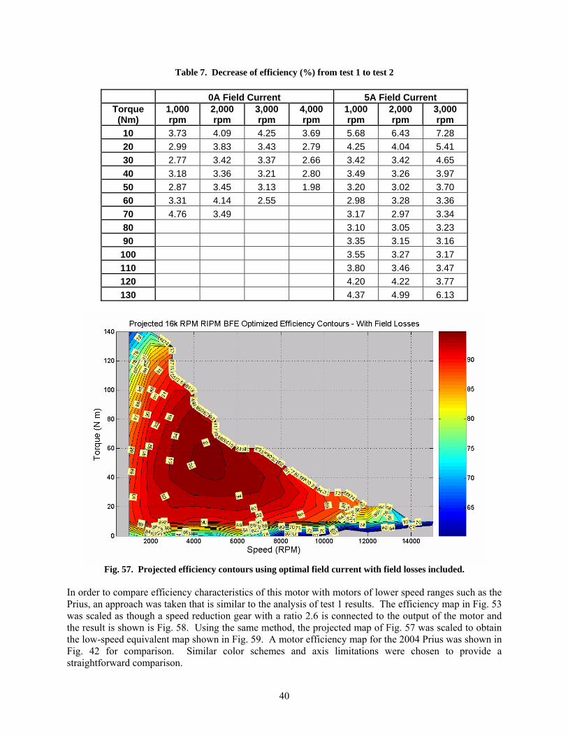
locked-rotor tests were not conducted. However, the torque-current ratio has a similar connotation for this assessment. The torque-current ratio with a field current of 5A for test 1 at 2900 rpm and test 2 at 3000 rpm is shown in Fig. 56. From test 1 to test 2, the average decrease of the torque-current ratio for speeds below 5000 rpm and field currents of 0A and 5A is between 4 and 5%, which is exceptionally close to the decrease observed in the back-emf voltage. This reaffirms that flux is inhibited more in the second stator than in the first stator. A comparison of motor efficiencies measured in each of the tests is provided in Table 7. The table shows the amount of efficiency decrease from test 1 to test 2, which is for the most part between 3 and 4%. Note that field losses are not included in the efficiencies list in Table 7. These correlations were incorporated with the efficiency data of test 2 in order to extrapolate an efficiency map for stator 1 over the entire speed range, which is shown in Fig. 57 and should be comparable at low speeds with Fig. 41. Note that the efficiency map of the second test series is lacking the low-torque peak efficiency regions, which are well defined in Fig. 41. For example, at 10 Nm and 2500 rpm, efficiencies reach 94% in test 1, but the efficiency only reaches about 88% in test 2, which is much greater than the average difference of 3–4%.

0

0.2

0.4

0.6

0.8

1

1.2

0 50 100 150

Torque (N m)

Torq

ue/C

urre

nt R

atio

(Nm

/Arm

s)

2900rpm Test13000rpm Test2

Fig. 56. Torque-current ratio for tests 1 and 2 at 5A.

40

Table 7. Decrease of efficiency (%) from test 1 to test 2

0A Field Current 5A Field Current Torque (Nm)

1,000 rpm

2,000 rpm

3,000 rpm

4,000 rpm

1,000 rpm

2,000 rpm

3,000 rpm

10 3.73 4.09 4.25 3.69 5.68 6.43 7.28 20 2.99 3.83 3.43 2.79 4.25 4.04 5.41 30 2.77 3.42 3.37 2.66 3.42 3.42 4.65 40 3.18 3.36 3.21 2.80 3.49 3.26 3.97 50 2.87 3.45 3.13 1.98 3.20 3.02 3.70 60 3.31 4.14 2.55 2.98 3.28 3.36 70 4.76 3.49 3.17 2.97 3.34 80 3.10 3.05 3.23 90 3.35 3.15 3.16

100 3.55 3.27 3.17 110 3.80 3.46 3.47 120 4.20 4.22 3.77 130 4.37 4.99 6.13

Fig. 57. Projected efficiency contours using optimal field current with field losses included.

In order to compare efficiency characteristics of this motor with motors of lower speed ranges such as the Prius, an approach was taken that is similar to the analysis of test 1 results. The efficiency map in Fig. 53 was scaled as though a speed reduction gear with a ratio 2.6 is connected to the output of the motor and the result is shown is Fig. 58. Using the same method, the projected map of Fig. 57 was scaled to obtain the low-speed equivalent map shown in Fig. 59. A motor efficiency map for the 2004 Prius was shown in Fig. 42 for comparison. Similar color schemes and axis limitations were chosen to provide a straightforward comparison.

41

Fig. 58. RIPM BFE efficiency map with field losses and gear ratio of 2.6.

Fig. 59. Projected RIPM BFE efficiency map with field losses and gear ratio of 2.6.

A comparison of Fig. 58 with Fig. 42 shows that the low-speed efficiency is slightly higher than the Prius efficiency in this region. The Prius has slightly broader contour areas for efficiencies above 90%, and significantly higher efficiencies at high speeds. These maps would look even more similar if a slightly smaller gear ratio were used. The projected efficiency map in Fig. 59 is substantially superior to the Prius efficiency map. Note As indicated in Fig. 41, that the efficiencies below 5,000 (or ~1,923 in Fig. 59) have been experimentally verified. Also, the high-speed efficiencies of stator 1 were likely to be higher than what is indicated in Fig. 58, since a modest method was used to generate the projected map.

42

VIBRATION ANALYSIS A vibration analysis obtained from testing is shown in Fig. 60. The vibration analysis test was not repeated over the higher speed range, because the motor was running smoothly at high speed.

Vibration vs Speed

0

0.01

0.02

0.03

0.04

0.05

0.06

0 1000 2000 3000 4000 5000 6000

Speed (RPM)

Velo

city

(Inc

hes/

seco

nd)

Fig. 60. Vibration analysis obtained from test.

43

CONCLUSIONS (1) This research effort proves that BFE from the third dimension (i.e. the axial direction) for an IPM

machine is practical and effective. The back-emf is easily controlled with an external field excitation current in the 0–5A range. The excitation dc voltage does not exceed 80 volts. This field excitation range is capable of changing the air-gap flux density up to 2.5 times at a given speed. This enables the motor to have the high power density advantage of conventional strong PM reluctance motors as well as the low back-emf and lower core loss advantage of weak PM reluctance motors. The circuitry required to supply the excitation current to the coils is projected to cost under $10 in production quantities.

(2) While the rotor is rotating at high speed with no field current, the core loss is significantly lower

than that of fixed PM motors. The core and friction loss test results show the benefits of lower air-gap flux density. For example, at 5000 rpm the core and friction loss is 200 W at zero field excitation, compared with 600 W at high field excitation for a high air-gap flux density. This should positively impact the highway fuel efficiency of the vehicle.

(3) The prototype motor design permits the rotor punching bridges to be thicker to satisfy the high

speed mechanical stress requirements. Due to this rotor design, flux produced by the PMs can leak through causing the air-gap flux density produced by the PMs to be reduced more than in similar IPM machines (such as the lower-speed baseline motor). The weaker air-gap flux density improves high-speed operation and can be compensated with BFE current for increased torque production at lower speeds.

(4) The rotor performed at high speed without failure. (5) The PM in the rotor acts as a flux barrier; thus, the air gap flux depends mainly on the adjustable

field excitation. The ideal PM property for the field excitation should be a high coercivity, Hc, and a relatively low remanence, Br. These would enhance the field adjustment ratio and lower the high speed core losses.

(6) If an interior short-circuit fault occurs in the windings, the excitation current can be cut off to

prevent inadvertently damaging the motor. (7) The RIPM-BFE motor benefits from using an optimal field current combined with the capability of

reducing the air gap flux when not needed. This results in increased efficiencies at low torques for both partial loads and high speeds. This can be confirmed by comparing Figs. 41 and 42 for the low speed region of the tests conducted prior to rewinding the motor. The projected RIPM-BFE motor performance from the rewound motor show greater efficiency advantages than those of the baseline (Prius) motor.

Although the rewound motor had a lower efficiency, the benefits of variable field excitation are still

clearly observed. (8) Rewound motor tests indicated a variable 2–5% drop in efficiency from the initial motor tests. It

was determined that the stator bore was enlarged by the winding fabricator during cleaning before rewinding. This was confirmed by lower back-emf results in subsequent testing. The original stator showed significant advantages, particularly in terms of motor efficiency, over motors of similar application and power level, such as the Prius. The efficiency map for the high speed region was projected from the test results of the rewound motor to indicate what the efficiency would be if the tests were conducted on the initial motor.

44

(9) An aluminum frame is used in the prototype design so as to not increase the weight of the field

excitation. (10) Test confirms that the asymmetrical rotor can increase the forward performance on the expense of

reducing the backward performance. However, further study on this topic is needed. (11) The RIPM-BFE motor should not present any manufacturing issues in mass production. Design

improvements on the excitation coils to motor housing interface will result in a reduction of both mass and volume of the prototype motor thereby reducing manufacturing costs.

(12) As a result of this research effort, a significant improvement in the development of accurate 3-D

finite-element simulations and a magnetically saturated lump parameter computational method for 3-D electric machine designs was achieved.

(13) The prototype motor is not the optimal possible design of a high speed motor that uses the 3-D field

excitation technology. It was initially designed to compare with the lower speed baseline (Prius) motor. Various improvement options learned from this project can be used to meet different design constrains.

45

REFERENCES

1. Munehiro Kamiya, “Development of Traction Drive Motors for the Toyota Hybrid System,” Toyota

Motor Corporation, 1, Toyota-cho, Toyota, Aichi, 471-8571, Japan. 2. Masaki Okamura, Eiji Sato, and Shoichi Sasaki, “Development of Hybrid Electric Drive System

Using a Boost Converter,” Toyota Motor Corporation, 1, Toyota-cho, Toyota, Aichi, 471-8572, Japan.

Patents: J. S. Hsu et al., Method for Providing Slip Energy Control in Permanent Magnet Electric Machines,

U.S. Patent No. 7,134,180, November 14, 2006. J. S. Hsu et al., Method and Radial Gap Machine for High Strength Undiffused Brushless Operation,

U.S. Patent No. 7129611, October 31, 2006. J. S. Hsu et al., Auxiliary Power Generation in a Motor Transformer, U.S. Patent No. 7,092,267,

August 15, 2006. G. J. Su et al., Integrated Inverter for Driving Multiple Electrical Machines, U.S. Patent No. 7,023,171,

April 4, 2006. J. S. Hsu et al., Rotor Apparatus for High Strength Undiffused Brushless Electric Machine, U.S. Patent

No. 6,989,619, January 24, 2006. J. S. Hsu et al., Hybrid-Secondary Uncluttered Permanent Magnet Machine and Method, U.S. Patent No.

6,977,454, December 20, 2005. J. S. Hsu et al., Permanent Magnet Machine and Method with Reluctance Poles for High Strength

Undiffused Brushless Operation, U.S. Patent No. 6,972,504, December 6, 2005. J. S. Hsu et al., Simplified Hybrid-Secondary Uncluttered Machine and Method, U.S. Patent No.

6,891,301, May 10, 2005. J. S. Hsu et al., High Strength Undiffused Brushless (HSUB) Machine, U.S. Patent No. 6,573,634,

June 3, 2003. J. S. Hsu et al., Hybrid Secondary Uncluttered Induction Machine, U.S. Patent No. 6,310,417,

October 30, 2001. J. S. Hsu et al., Permanent Magnet Energy Conversion Machine, U.S. Patent No. 5,952,756,

September 14, 1999.

46

APPENDIX: ADDITIONAL SECOND SERIES TEST EFFICIENCY MAPS

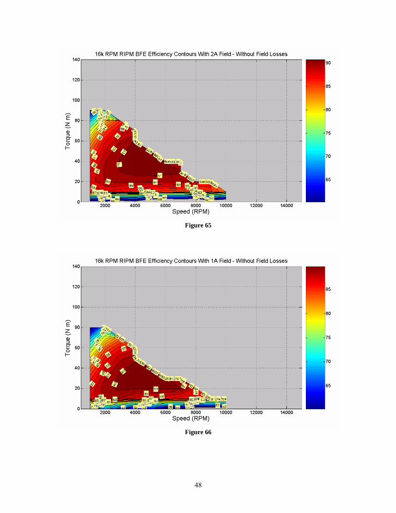
OF 16,000-RPM RIPM BFE REWOUND MOTOR Efficiency Maps without Field Losses Included (Figs. 61–67).

Figure 61

Figure 62

47

Figure 63

Figure 64

48

Figure 65

Figure 66

49

Figure 67

Efficiency Maps with Field Losses Included

Figure 68

50

Figure 69

Figure 70

51

Figure 71

Figure 72

52

Figure 73

Figure 74

53

DISTRIBUTION

Internal

1. D. J. Adams 2. T.A. Burress 3. C. L. Coomer 4. E. C. Fox 5. K. P. Gambrell 6. J. S. Hsu

7. S. T. Lee 8. L. D. Marlino 9. J. H. McKeever

10. M. Olszewski 11. R. H. Wiles 12. Laboratory Records

External

13. R. Al-Attar, DCX, raa9@dcx.com. 14. T. Q. Duong, U.S. Department of Energy, EE-2G/Forrestal Building, 1000 Independence

Avenue, S.W., Washington, D.C. 20585. 15. R. R. Fessler, BIZTEK Consulting, Inc., 820 Roslyn Place, Evanston, Illinois 60201-1724. 16. K. Fiegenschuh, Ford Motor Company, Scientific Research Laboratory, 2101 Village Road,

MD-2247, Dearborn, Michigan 48121. 17. V. Garg, Ford Motor Company, 15050 Commerce Drive, North, Dearborn, Michigan 48120-

1261. 18. G. Hagey, Sentech, Inc., 501 Randolph St., Williamsburg, Virginia 23185. 19. E. Jih, Ford Motor Company, Scientific Research Laboratory, 2101 Village Road, MD-1170,

Rm. 2331, Dearborn, Michigan 48121. 20. K. J. Kelly, National Renewable Energy Laboratory, 1617 Cole Boulevard, Golden, Colorado

80401 21. A. Lee, Daimler Chrysler, CIMS 484-08-06, 800 Chrysler Drive, Auburn Hills, Michigan 48326-

2757. 22. F. Liang, Ford Motor Company, Scientific Research Laboratory, 2101 Village Road, MD1170,

Rm. 2331/SRL, Dearborn, Michigan 48121. 23. M. W. Lloyd, Energetics, Inc., 7164 Columbia Gateway Drive, Columbia, Maryland 21046. 24. M. Mehall, Ford Motor Company, Scientific Research Laboratory, 2101 Village Road, MD-2247,

Rm. 3317, Dearborn, Michigan 48124-2053. 25. J. A. Montemarano–Naval Surface Warfare Center, Carderock Division; Code 642, NSWCD,

9500 MacArthur Boulevard; West Bethesda, Maryland 20817 26. N. Olds, United States Council for Automotive Research (USCAR), nolds@uscar.org 27. J. Rogers, Chemical and Environmental Sciences Laboratory, GM R&D Center, 30500 Mound

Road, Warren, Michigan 48090-9055. 28. S. A. Rogers, U.S. Department of Energy, EE-2G/Forrestal Building, 1000 Independence

Avenue, S.W., Washington, D.C. 20585. 29. G. S. Smith, General Motors Advanced Technology Center, 3050 Lomita Boulevard, Torrance,

California 90505. 30. E. J. Wall, U.S. Department of Energy, EE-2G/Forrestal Building, 1000 Independence Avenue,

S.W., Washington, D.C. 20585. 31. B. Welchko, General Motors Advanced Technology Center, 3050 Lomita Boulevard, Torrance,

California 90505. 32. P. G. Yoshida, U.S. Department of Energy, EE-2G/Forrestal Building, 1000 Independence Avenue,

S.W., Washington, D.C. 20585.