15.997 Practice of Finance: Advanced Corporate Risk Management · 2020-01-04 · 15.997 Practice of Finance: Advanced Corporate Risk Management ... Some students will be familiar

MIT OpenCourseWarehttp://ocw.mit.edu

15.997 Practice of Finance: Advanced Corporate Risk Management Spring 2009

For information about citing these materials or our Terms of Use, visit: http://ocw.mit.edu/terms.

http://ocw.mit.edu

http://ocw.mit.edu/terms

Lecture Notes on Advanced Corporate Financial Risk Management John E. Parsons and Antonio S. Mello

Chapter 6: Measuring Risk–Dynamic Models

Part A—The Random Walk Model of Stock Prices

Recent decades have witnessed revolutionary advances in the tools used to model risk

and to price risky financial assets. The Black-Scholes-Merton approach to option pricing has been

generalized to all corporate liabilities, including stocks, bonds and derivatives of all types. This

approach is now commonly used to price mortgage obligations, currency agreements, insurance

contracts and myriad other financial instruments. Most recently, the approach has been extended

to the valuation of real options, investments in real assets such as the development of oil fields,

the operation of electric generating plants and the negotiation of options to purchase aircraft.

The engine under the hood of every real options model is a stochastic process model of

one or more critical variables or factors—the oil price, for example. A stochastic process model is

a parsimonious description of the dynamics governing the evolution of the variable through time.

It captures long-term trends—such as any forecasted long-term increase in the price. It captures

short-term dynamics such as seasonal fluctuations, as well as the tendency of sudden price shocks

to reverse themselves. And it captures all elements of uncertainty, both short-term shocks that are

dissipated and long-term shocks that persist and are compounded. Once the stochastic process

model is specified and its parameters estimated, an analyst can value all varieties of real assets

with cash flows tied in any complicated way to the factor.

How well the engine runs depends upon what you put in it. If the model accurately

captures the dynamics—both in general structure, as well as in the precise values of the

parameters—then the risk assessment and valuations made using the model will be useful. If the

model is inaccurate, then, …well, then we have a problem. So it is critical for the corporate

manager to understand the essential characteristics of alternative models and be able to evaluate

the fidelity of the model to the dynamics of the factors and risks driving their business.

Chapter 6: Measuring Risk—Dynamic Models

This chapter is predicated on a distinction between the underlying factor and the

derivative asset. First we model the underlying factor. Then we determine how the cash flows or

value of an asset is derived from this underlying factor – hence the term ‘derivative’. Then we try

to understand how the risk from the underlying factor is translated into risk for the asset.

Some students will be familiar with the tools here as developed for modeling stocks and

other financial instruments. Our analysis is meant to apply more generally. Any variable can

conceivably be a factor, and we need to think about the many ways that risk should be modeled

for the full diversity of variables that can be factors. Because our analysis is meant to be very

general, students should be cautious about applying all of the results learned in the context of

modeling financial assets. The equilibrium conditions determining the prices of financial assets

impose specific conditions on the models used. Since we are modeling general variables, not just

financial assets, the equilibrium conditions may not apply and the models may have properties

different from what the student is familiar with.

In this chapter we have tried to strike a difficult balance. We present the bare essentials of

stochastic process modeling, attempting to minimize the mathematical detail, while still providing

enough material to enable the reader to actually implement and evaluate these models. We

present a broad selection of models which embody very different structures of risk and which we

believe give the reader a good feel for the various risk patterns that can be modeled. But, of

course, the full library of potential models is much larger, and the true specialist will know that

we have only touched the surface. We have tried to select models that we believe provide a useful

representation of relevant factors—for example, a good model of the oil price that can be reliably

used to assess the risk of major oil related capital investments. In doing so, we have chosen to

brush aside aspects that we believe are of lesser significance for corporate managers, although

they may be significant for short-term money managers speculating on oil futures. All of these

choices involve judgment and reasonable people may differ. This is our best shot.

6.1 Discrete Time Stochastic Process

We start with the standard discrete time stochastic process model for stock prices, the

random walk model. Suppose that we want to analyze a stock with an average annual return of

μ=12%, also known as the drift, and volatility σ=22%. Suppose further that we are analyzing the

stock’s possible movement through the horizon T=2. We divide this into N total periods or n

periods per year, n=N/T, where the length of each period is Δt=1/n. If n=12, then each period is a

page 2


month and Δt=0.0833, if n=52, then each period is a week and Δt=0.0192, if n=250, then each

period is a trading day and Δt=0.0040, and so on. We mark off the N points in time as t0, t1 …

ti,… tN, with t0=0 and tN=T. Figure 6.1 below illustrates this structure.

The initial stock price, S(t0), is given. The return earned over the period from t0 to t1,

R(t1), and therefore the next period stock price, S(t1), are random variables. We define the return

as the continuously compounded return so that:

S(ti ) = S(ti−1)eR (ti ) , (6.1)

or equivalently,

R(ti ) = ln⎜⎜⎛

⎝ SS (( tt

i−

i

1

)) ⎟⎟⎞

⎠ = ln(S(ti ))− ln(S(ti−1)) . (6.2)

An important property of continuously compounded returns is that they are additive: the

cumulative return over any horizon, R(t0,ti), is equal to the sum of the returns over that horizon.

One can see this by analyzing the recursive calculation of the price:

S(t1) = S(t0 )eR (t1)

and

S(t2 ) = S(t1)eR (t2 ) ,

therefore

S(t2 ) = S(t0 )eR (t1) eR (t2 ) ,

or, equivalently

S(t2 ) = S(t0 )eR (t1)+R (t2 ) ,

which, by definition, is the cumulative return,

S(t2 ) = S(t0 )eR (t1,t2 ) .

This recursive substitution can be repeated any number of periods. Therefore, we are free to write

i

R(t0 ,ti ) = ∑R( ) tk (6.3) k=1

page 3


and,

S(ti ) = S(t0 ) eR(t0 ,ti ) . (6.4)

We assume each return is an independently and identically distributed random variable

from a normal distribution with mean m and variance v2:

R(ti ) = m + v ε~ i (6.5)

where εi is a standard normal random variable. The mean and variance of the period return

depend on the size of the period, Δt. In order that the annual return and variance equal μ and σ as

assumed above, we set m and v as follows:

1 2m(Δt) = (μ − 2 σ )Δt , (6.6)

v(Δt) =σ Δt . (6.7)

The rationale for this definition will become clear shortly.

6.2 Monte Carlo Simulation

We can easily simulate this stochastic process. First we need a series of N draws of the

standard normal random variables, ε1, ε2, … εN, which can be readily generated in a standard

Excel spreadsheet or with any of a number of other mathematical programs. We then calculate the

N return variables R(t1), R(t2), … R(tN) using equation (6.5), and then calculate the N cumulative

return variables, R(t0,t1), R(t0,t2), … R(t0,tN) using equation (6.3) and the N stock price variables,

S(t1), S(t2), … S(tN) using equation (6.4). This gives us a sample path for the stock price.

Table 6.1 shows a sample of the first 10 draws of the standard normal random variable

and the calculation of returns, cumulative returns and stock prices assuming input parameters

μ=12% and σ=22% and periods of a week’s length, n=52 and Δt=0.0192. For these parameters

we have m=0.18% and v=3.05%.

Figure 6.2 shows how a sample path of the stock price series might appear given three

different choices for the length of a period—one month, one week and one trading day.

Figure 6.3 shows 4 different sample paths of the stock price generated by the same

parameters, but using different sets of draws of the standard normal random variables, ε1, ε2, …

εN. Also shown in Figure 6.3 are the corresponding sample paths of cumulative returns.

page 4


In constructing our simulation, we used the intermediate step of calculating cumulative

returns and then stock prices, when it would have been possible to move directly from returns to

stock prices by applying equation (6.1) recursively. There are a number of reasons why it is

useful to construct our simulation and perform much of the analysis in cumulative returns instead

of directly in terms of stock prices. Once we have constructed the cumulative return at any

horizon, it is a simple matter to translate that back into a stock price. One reason for working in

returns is that the scale is invariant. In a graph of cumulative returns, a five percentage point

change looks the same, regardless of whether it is a five percentage point change from a low

cumulative return or from a high cumulative return. In a graph of stock prices, a five percentage

point change looks smaller if it is a change from a low stock price and looks larger if it is a

change from a high stock price. Since stock prices tends to grow exponentially, this tends to

exaggerate the significance of later returns as compared to earlier returns and distorts our ability

to grasp the dynamics. Working in returns is also useful in minimizing the impact of the rounding

errors that creep into calculations with many periods. The cumulative impact of these errors is

smaller if we first sum returns and only exponentiate the cumulative return at the conclusion of

the analysis in order to translate the results back into stock prices.

By generating repeated paths of the series of returns and stock prices we can produce a

histogram of values for the stock price and the cumulative return at any point in time, t∈{t1 …

ti,… tN}. Figure 6.4 shows a histogram of cumulative returns for a simulation of 100 sample paths

over a horizon of T=2 years using N=100 periods in total or n=50 per year, with μ=12% and

σ=22%.

For a large enough set of paths, this histogram should approximate the true probability

distribution for the process we are simulating, and so can be used to estimate an answer for

certain standard types of probability questions. What is the expected cumulative return to T=2? In

this small sample, the mean cumulative return at T=2 is 21.2%. What is the standard deviation of

cumulative returns at T=2? The sample standard deviation is 28.1%. What is the probability that

the stock price at 2 years is greater than $90? In our small sample, 86% of the paths end with a

stock price greater than $90 at T=2. What is the expected stock price at T=2, given that it is

greater than $90? In our sample, the average stock price at T=2 among those paths for which the

price is greater than $90, is $136.62. What is the probability that between t=0 and t=T the price is

always above $90 within the 2 year horizon? In our sample, 46% of the paths are always above

page 5


$90 throughout the entire window. As tedious as these types of calculations are, they are

nevertheless readily doable with a computer.

Obviously, the accuracy of our estimated answers to these questions depends upon the

size of the sample we take. A sample of 100 is useful for getting an initial feel for a problem, but

is far too small for reliable results on any interesting questions. It is common to see results

presented using a sample size of 10,000 runs, but there is nothing sacrosanct about this number.

The right sample needed depends upon the degree of accuracy required and the particular

function being estimated. The accuracy also depends on other elements of the simulation. For

example, the formula and procedure used to generate the random number can affect the accuracy.

Also, it should be clear that simply reproducing the distribution in the way we have described—

simple sampling—is a sort of brute force technique. A number of techniques have been

developed to deliberately select a sample that most efficiently reflects the properties of the

underlying distribution, i.e., using the smallest sample size. See, for example, Latin hypercube

sampling or orthogonal sampling. These techniques will not be explored in any more detail here.

More important than the size or technique of sampling, of course, is the question of

whether the mathematical model we are using is the right one and whether the parameter values

we have selected are right. As always, we are subject to the dictum ‘garbage in, garbage out.’

6.3 The Normal Distribution of Returns

Earlier we assumed that each period’s return was normally distributed and that each

period’s return was independently and identically distributed. This will give us a simple

expression for the probability distribution of returns at every horizon, which in turn will enable us

to derive explicit formulas for the types of questions we had asked earlier, questions about the

likely and conditional values of the stock price and returns.

The sum of a set of normal random variables is itself normally distributed. Because the

returns each period are independently distributed, the mean of the sum is the sum of the means.

And because they are identically distributed, the sum of the mean returns is simply proportional

to the number of periods, i, or elapsed time, ti:

[ ( )] = E⎡ i

R t ⎤=

i

E[R( )t ] = i

m = miE R t0 ,t ( ) .i ⎢∑ k ⎥ ∑ k ∑⎣ k=1 ⎦ k=1 k=1

page 6


Noting that the mean return in a single period, m, is actually a function of the length of the period,

m(Δt), we can rewrite this as

1 2 1 2E R t0 ,ti ( 2 ( . (6.8)[ ( )] = m(Δt)i = μ − σ )Δt i = μ − 2 σ )ti

The assumption of independently distributed returns also implies that the variance of the

sum of returns is equal to the sum of the variances of the returns. And since the returns are

identically distributed, the variance of the sum of returns is also linear in the number of periods, i,

or elapsed time, ti:

2 2[ ( )] =Var⎡ i

R t ⎤=

i

Var[R( )t = i

v = v iVar R t0 ,ti ⎢∑ ( )k ⎥ ∑ k ] ∑ . ⎣ k=1 ⎦ k=1 k=1

Noting that the standard deviation of the return in a single period, v, is actually a function of the

length of the period, v(Δt), we can rewrite this as

[ ( )]= v(Δt) i =σ Δt iVar R t0 ,ti 2 2 =σ 2 ti . (6.9)

Therefore, the cumulative return from period 0 to period i is normally distributed, with mean mi

and variance vi2:

R(t0,ti) ~ N(mi,v2i),

or, equivalently, the cumulative return from period 0 to period i is normally distributed, with

mean (μ–½σ2)t and variance σ2t:

1 2 2R( )t0 ,ti ~ N ((μ − 2 σ )ti ,σ ti ).

The top panel of Figure 6.5 shows the probability distribution of cumulative returns over

a horizon of T=2 years with μ=12% and σ=22%. It should be compared against the histogram of

returns shown in Figure 6.4. The mean of the distribution is a return of 19.2%. This should be

compared against the mean in the sample which was 21.2%. The difference between those two

values reflects the error we get because our small sample turns out not to be wholly representative

of the full distribution. The larger the sample size the smaller this error is likely to be. The

standard deviation of the distribution shown in Figure 6.5 is 31.1%. This should be compared

against the standard deviation of the sample which was 28.1%.

page 7


The top panel of Figure 6.6 shows the expected cumulative return at each horizon using

equation (6.8). Also shown are the one standard deviation confidence bounds which correspond

to the 68% confidence interval using these equations:

1UR(t0,ti) = (μ − 2 σ 2 )ti + σ ti (6.10)

1LR(t0,ti) = (μ − 2 σ 2 )ti −σ ti . (6.11)

One can see in the figure as well as in equation (6.8) that the expected cumulative return grows

linearly in time. One can see in equation (6.9) that the variance of return also grows linearly in

time. This means that the standard deviation or volatility of return grows as the square root of

time, and one sees this in the shape of the confidence bounds graphed in Figure 6.6 and in the

form of equations (6.10) and (6.11).

6.4 The Lognormal Distribution of Prices

The expected value and variance of the stock price variable is slightly more complicated

since the stock price is equal to the exponentiated return. Rewriting the relationship between the

stock price and returns shown in equation (6.2) we have

ln(S(ti )) = ln(S(ti−1)) + R(ti )

~ = ln(S(ti−1)) + m + vε i . (6.12)

Since the return is a normally distributed random variable, equation (6.12) implies that

the log of the price is normally distributed. In that case, the price itself is lognormally distributed:

S(ti) ~ Log-N (ln(S(ti−1) + m,v2 ),

or, alternatively,

1 2 2S(ti) ~ Log-N (ln(S(t0 ) + (μ − 2 σ )ti ,σ ti ) .

The bottom panel of Figure 6.5 shows a lognormal distribution. Contrast the normal

distribution of cumulative returns shown in the top panel of Figure 6.5 with the lognormal

distribution of prices. A lognormally distributed random variable can never go below zero, which

is an appropriate feature for a distribution describing stock prices. But this contributes to the fact

that the lognormal is not a symmetric distribution. It is skewed to the left, with a long upper tail.

Consequently, the median of the distribution will lie to the left of the mean, which is an important

page 8


property in understanding the relationship between expected returns and expected prices. The

mean return in the top panel is also the median return. Looking back at the bottom panel of Figure

6.3, the histogram of stock prices from our Monte Carlo simulation, you can see the features of a

lognormal distribution there, too, and you can contrast these with the features of the normal

distribution in the histogram of stock returns immediately above it.

Standing at t0, the expected value of the stock price at t1, S(t1), is given by:

2E(S(t1)) = S(t0 ) em+ 1v2

.

Note that the volatility parameter, v, enters into the expectation, increasing the expected

value. Consequently, the expected stock price is greater than the price corresponding to the

expected return:

E(S(t1)) = S(t0 ) em+ 12v2

> S(t0 ) em = S(t0 ) eE ( R(t1)) .

This is because the variance component of the return makes its own contribution to the expected

stock price:

E(S(t1)) = E(S(t0 )eR (t1) ) = E(S(t0 ) em+vε~1 ) = S(t0 ) em E(evε~ i ) .

Although the mean of the random term ε1 is zero, the expected value of the exponentiated random

term is not zero:

vε~1 2vE(e ) = e 1 2

.

The expected stock price through time is therefore given by

⎜m+ v ⎟i⎝ 2 ⎠E(S(ti )) = S(t0 ) e ⎛ 1 2 ⎞

.

Noting that the mean return in a single period, m, is actually a function of the length of the period,

m(Δt), we can rewrite this as

⎝ 2 2 ⎠ μ tiE(S(ti )) = S(t0 ) e ⎜⎛ μ− 1σ 2+ 1σ 2 ⎟⎞ti = S(t0 ) e . (6.13)

Our earlier choice of parameterization for the per period mean return, writing 1 2m(Δt) = (μ − σ )Δt , allowed us here, in calculating the mean price, to cancel the terms where 2

the volatility enters and obtain an expression exclusively in terms of the single parameter, μ.

page 9


The bottom panel of Figure 6.6 graphs the expected stock price through time from

equation (6.13). Also graphed is the median stock price, which is the price corresponding to the

median return given in equation (6.8):

⎛ − ⎞ ⎝ 2 ⎠S(t0 ) e ⎜ μ 1σ 2 ⎟ti . (6.14)

The median stock price is always less than the mean stock price. Finally, the bottom panel of

Figure 6.5 also graphs the upper and lower bounds on the 68% forecast confidence interval for

the stock price. These are calculated by exponentiating the upper and lower bounds confidence

interval for returns in equations (6.10) and (6.11):

US(ti ) = S(t0 )eUR(t0 ,ti ) , and (6.15)

LS (ti ) = S(t0 )eLR (t0 ,ti ) . (6.16)

6.5 Probability Calculations

Earlier, we used Monte Carlo simulation to estimate answers to questions such as, what is

the probability that the stock price at T=2 is greater than $90? Monte Carlo simulation is a very

empirical way to approach this question, but one that requires the brute force of many

calculations to implement. Because we now have a convenient characterization of the distribution

of prices at every horizon, we can directly derive the precise answer to this question without

going through the full simulation process. We start by noting that S(ti)>X exactly when

ln(S(ti))>ln(X), so that:

Pr(S(ti ) > X ) = Pr(ln(S(ti )) > ln(X ))

Since ln(S(ti) is normally distributed, if we subtract the mean and divide by the standard

deviation, we will transform it to a standard normal random variable for which the relevant

probabilities are readily to hand. Doing this to both sides of the expression inside the probability

function gives us:

ln(S(ti )) ( S(t ) − μ − σ )t ln X − ln S t )− ( −⎛ − ln 0 ) ( 12

2 i ( ) ( ( 0 ) μ 1

2 σ2 )ti

⎞ = Pr⎜⎜

⎝ σ ti

>σ ti

⎟⎟⎠

= Pr ⎛⎜⎜ z >

ln( ) ( X − ln S(t0 ))− (μ − 12 σ

2 )ti ⎞⎟ ,

⎝ σ ti ⎟⎠

page 10


where z is a standard normally distributed random variable. Taking advantage of symmetry

around zero in the standard normal distribution, we can rewrite this as

ln( ) ( − ln S t )− (μ − σ )t = Pr⎜⎜

⎛

⎝ z < −

X ( σ

0 ) ti

12

2 i

⎟⎟⎞

⎠

ln( ( )) ( )ln X + ( − σ ) ⎞ = Pr⎜

⎛ z <

S t0 − μ 12

2 ti ⎟ ⎜ σ ti

⎟⎠⎝

= N ⎛⎜ (S(t )) ( )ln + ( − 1

2 σ2 )t ⎞⎟ ,

ln 0 − X μ i

⎜ σ ti ⎟⎠⎝

where N( ) is the cumulative normal distribution function. The expression inside the parenthesis is

of a form that appears in the Black-Scholes equation for the price of a call option. Black-Scholes

used the variable d2 for this expression. Since our expression is similar, but slightly different, we

will use the variable d̂2 :

1 2 ˆ ln(S(t0 ))− ln(X )+ (μ − 2 σ )tid2 = , (6.17)

σ ti

so that we have

Pr(S(ti ) > X ) = N (d̂2 ). (6.18)

We can solve for the complementary probability that the price ends up below the value X,

Pr(S(ti ) < X ) = N (− d̂2 ) . (6.19)

We will come back to analyze the expression for d̂2 in more detail when we come to pricing risk

and the valuation of a call option. We can evaluate equations 6.18 and 6.19 in Excel using the

NormSDist function. For our assumed parameters of T=2 years, μ=12% and σ=22%, we have

d̂2 =0.95447 and we arrive at the solution that Pr(S(ti)>X)= 83%. This should be contrasted with

the value of 86% from our Monte Carlo simulation.

Earlier we had also asked, what is the expected stock price at T=2 given that it is greater

than $90? This, too, can be given a precise answer without resort to simulation.

page 11


∞ ∞

E[S(ti ) S(ti ) > X ] = ∫ S(ti ) f (S(ti )) dS(ti ) ∫ f (S(ti )) dS(ti ) X X

⎛ X μ 1 2 ⎞ = S(t0 ) eμ ti N⎜ ln(S(t0 ))− ln( ) + ( + 2 σ )ti ⎟ N d̂2( )⎜ σ ti

⎟⎠⎝

= S(t ) eμ ti N (d̂ ) N (d̂2 ) (6.20)0 1

where,

1 2 ˆ ln(S(t0 ))− ln(X )+ (μ + 2 σ )ti ˆd1 = = d2 +σ ti . (6.21)

σ ti

The variable d̂1 is also comparable to the variable d1 which appears in the Black-Scholes

equation. More on that later. Using equations 6.20 and 6.21, in our numerical example, we have

d̂1 =1.26559 and the expected stock price at T=2 given that it is greater than $90 is $137.40.

6.6 Estimating the Parameters

Until now, we have assumed a given stochastic process driving the evolution of the stock

price, and we have assumed values for the pair of parameters defining that process, μ and σ. Then

we have generated probabilistic forecasts of what realization of stock returns and prices we would

be likely to see. In reality, neither the process nor the parameters are given. We observe a history

of past stock returns and prices, and we infer the structure of the process, including the values for

the parameters μ and σ.

For the moment, we are going to continue with the assumption that we know the general

structure of the stochastic process driving returns and prices. However, we are going to

acknowledge that we do not necessarily know the values for the parameters μ and σ. How do we

estimate the parameters μ and σ from a history of stock price data?

One of the attractive things about the stochastic process model we have been using is that

the estimation of the two parameters is very simple. Given a sample of N+1 stock price variables,

S(t0), S(t1), S(t2), … S(tN) we first calculate the sequence of N return variables R(t1), R(t2), …

R(tN), where R(ti)=ln(S(ti))/ln(S(ti-1)). Now we recall that the per period expected return is m, and

page 12


the volatility in per period returns is v. Estimates for m and v are simply the sample mean return

and sample standard deviation of returns:

N

ˆ ∑R tim = Mean = R = ( ) N , (6.22) i=1

N

∑( ( ) )v̂ = StDev = R ti − R 2 (N −1) . (6.23) i=1

Recalling that these estimators have been calculated from returns calculated over periods of

length Δt=1/n, whereas the parameters μ and σ are denominated as annual values, we need to

annualize the results by multiplying times the number of periods. In addition, we have to take

care to adjust the mean return estimator with one-half the variance:

μ̂ = (m̂ + 12 σ̂ 2 ) n , (6.24)

σ̂ = v̂ n . (6.25)

Table 6.2 shows the estimation of μ and σ based on a short sample of observed stock

prices. Because the sample is so short, both estimates have significant error. A larger number of

observations is obviously required.

There are two ways to obtain a larger number of observations: (i) observe the price more

frequently, increasing n and decreasing the length of a period, Δt, while keeping the horizon, T,

constant, or (ii) extend the horizon, T, keeping the length of a period, Δt, constant. Increasing the

frequently of observations, increasing n, and decreasing the length of a period, Δt, improves the

precision of the estimate of volatility, but does not improve the precision of the estimate of drift.

Extending the horizon improves the precision of the estimate of both drift and volatility, but it

improves the precision of drift most. Nevertheless, a good estimate of the drift generally takes a

very long horizon of data.

An intuitive way to understand why increasing the frequency of observations improves

the precision of the estimate of volatility, but not of drift, and to understand why increasing the

horizon is most useful for improving the estimate of drift is to examine the portion of a single

period’s return determined by each: Look at the ratio of the standard deviation of the return in a

period, v(Δt) to the mean return:

page 13


v(Δt) σ Δt σ x = = m(Δt) (μ − 1

2 σ 2 )Δt = (μ − 1

2 σ 2 ) . Δt

As the length of the period becomes very short, with Δt approaching zero, this ratio goes to

infinity. This means that what we observe in a very, very short period reflects volatility. As the

length of the period grows, with Δt approaching infinity, this ratio goes to zero, so that the

majority of what we are observing reflects the drift. Unfortunately, it takes a long time to get to

infinity, so it is difficult to get the information that we would like on the drift. It is much easier to

make more frequent observations and improve our estimate of volatility. In theory, greater and

greater frequency of observations will eventually give us a perfectly precise estimate of volatility.

In practice, there are extra elements of noise in frequent observations – such as bid-ask bounce or

a lack of trading, or simply mis-reporting of data – which put a limit on the value of the extra

frequency of observations and a bound on how precise can our estimates of volatility become. We

abstracted from these extra elements of noise when we structured the assumptions of our model.

6.7 The Continuous Time Representation

In the previous material, we modeled the stock price as a discrete time stochastic process.

Each year was divided into n periods of length Δt. Suppose we increase the number of periods a

year, letting the length of each period get smaller and smaller. If we continue this to the limit, so

that Δt is infinitesimally small, then we have a continuous process. We can write the process two

ways. The first is directly in terms of the stock price:

dSS(

( tt )) = μ dt + σ dz , (6.26)

The term dS(t) is the continuous time equivalent of the per period change in price, S(ti)-S(ti-1). The

term dt is the continuous time equivalent of Δt. The term dz is the continuous time equivalent of

the standard normal random variables, εi. However, this simple statement hides the very

complicated mathematical properties embedded in it. The term dz is called the Brownian motion.

The key feature of the Brownian motion is that variation in the value of the process are normally

distributed with a variance that is proportional to the length of the time period. Although the

volatility parameter in equation (6.26) does not, on its face, appear to be multiplied times the

square root of the time period—there is no dt multiplying the σ—this is only because the time

element is implicit in the Brownian motion term, dz.

page 14


This second way to write this process is in terms of the log of the price, i.e., in terms of

the returns:

1 2d ln(S(t)) = (μ − σ )dt + σ dz , (6.27)2

All of the properties we derived earlier for the discrete time process apply as well to this

continuous time version. Returns are normally distributed, with the mean and variance of the

return proportional to the horizon over which the return is compounded. Stock prices are

lognormally distributed, and the expected stock price at t is S0 eμ. All of the earlier functions for

the expected price and returns, confidence bounds and probability distributions remain valid.

Continuous time models are very mathematically demanding to develop and manipulate.

But the investment often pays off since the mathematics enables development of powerful

insights that can be difficult to grasp as readily when working in discrete time. Nevertheless, it is

beyond the scope of this book to provide the reader with the tools necessary to work directly in

continuous time. Instead, we simply exploit the continuous time results that have been produced

and published in the literature, without attempting to derive them here. And we will try to make

clear the correspondence between a given continuous time model and an alternative discrete time

representation so that the reader develops the ability to perform as an intelligent consumer of

future results in continuous time mathematics. In general, we will limit ourselves in this book to

implementing solutions and simulations using discrete time processes, even where we regularly

report on a particular continuous time model.

6.8 The Binomial and Other Tree or Lattice Representations

In this section we present a third way to model the random walk process, made popular

by one well known binomial version. The general idea is to represent the evolution of the price

through a series of branches in a tree. As with the discrete time stochastic process model, the

model hypothesizes a series of discrete steps that can be specified as longer or shorter time

intervals. However, at each point in time there are only a finite number of possible outcomes—in

the binomial model, unsurprisingly, just two. With a large enough number of steps, the final

distribution is very dense, despite the narrow range at each instant.

Using a tree structure has a couple of benefits. One is pedagogical. By reducing the

number of possible outcomes at each time, it is possible to describe very simply the key value

page 15


relationships from period to period. This makes the solutions transparent and easy to understand.

Therefore the binomial model has become a popular teaching tool.

Second, using the tree structure expands the range of valuation problems we can tackle.

Valuation is inherently forward looking and requires understanding the full structure of future

contingencies. Current values are calculated by discounting future cash flows. In this sense,

valuations starts from the end in time and moves backwards. To know today’s value, we first

need to know the distribution of possible values at the end of one year and then work backward.

The Monte Carlo method works the other ways around. It starts from the current parameter value

and generates a distribution for later dates. This works well for the single parameter being

simulated, for which the governing stochastic process has been exogenously specified. But it

doesn’t work well for determining the value of assets with cash flows that are tied to that

underlying parameter. With a binomial tree, once we know how the underlying parameter value

evolves along the nodes of the tree, we can also work backwards and calculate the values of an

asset with cash flows tied to that underlying parameter, and we can then learn how the value of

that asset evolves through time.

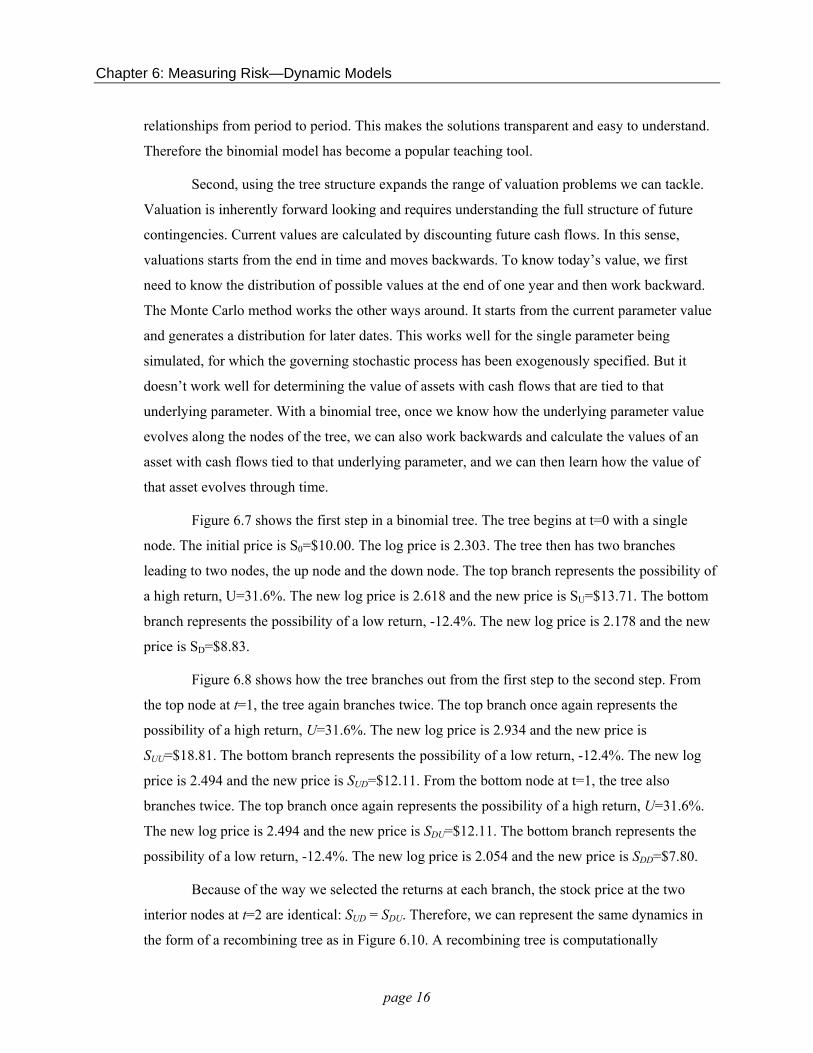
Figure 6.7 shows the first step in a binomial tree. The tree begins at t=0 with a single

node. The initial price is S0=$10.00. The log price is 2.303. The tree then has two branches

leading to two nodes, the up node and the down node. The top branch represents the possibility of

a high return, U=31.6%. The new log price is 2.618 and the new price is SU=$13.71. The bottom

branch represents the possibility of a low return, -12.4%. The new log price is 2.178 and the new

price is SD=$8.83.

Figure 6.8 shows how the tree branches out from the first step to the second step. From

the top node at t=1, the tree again branches twice. The top branch once again represents the

possibility of a high return, U=31.6%. The new log price is 2.934 and the new price is

SUU=$18.81. The bottom branch represents the possibility of a low return, -12.4%. The new log

price is 2.494 and the new price is SUD=$12.11. From the bottom node at t=1, the tree also

branches twice. The top branch once again represents the possibility of a high return, U=31.6%.

The new log price is 2.494 and the new price is SDU=$12.11. The bottom branch represents the

possibility of a low return, -12.4%. The new log price is 2.054 and the new price is SDD=$7.80.

Because of the way we selected the returns at each branch, the stock price at the two

interior nodes at t=2 are identical: SUD = SDU. Therefore, we can represent the same dynamics in

the form of a recombining tree as in Figure 6.10. A recombining tree is computationally

page 16


convenient since the number of nodes grows linearly with the number of period, whereas in the

non-recombining tree the number of nodes grows exponentially. However, there will be cases in

which a recombining tree is not useful since information about the history of returns is lost. More

on this later.

At first glance, a binomial tree appears too crude to adequately represent the risk

structure we used earlier to model a stock price. But the tree can be expanded to include many

more steps, and in that case the final branchings are a very dense representation of the range of

possible future stock prices. Figure 6.11 shows a recombining binomial tree with N=24 time

steps.

In the illustrations shown so far, we carefully selected the high and low returns for the

purpose of generating stock returns that are approximately normally distributed. Figure 6.11

shows the probability distribution across the final node of the tree. You can see that this

distribution is approximately normal. There are several different ways to define the returns and

probabilities along the tree so as to assure that the distribution across nodes is approximately

normal. In these lecture notes our default method will be to set the up node as one standard

deviation above the expected value and the down node as one standard deviation below the

expected value.1 The probability of following either path will be ½. In this example, with μ=9%,

σ=22%, and Δt=1 we have:

E[ln(S1)] = ln(S0)+(μ− 1/2σ2)Δt = 2.398,

so that

1 2ln(SU)= ln(S0 )+ (μ − 2 σ )Δt +σ Δt = 2.618

ln(SD)= ln( )+ ( − σ )Δt −S0 μ 12

2 σ Δt = 2.178.

We repeat this process at the subsequent nodes. Starting from t=1, at the top node where S1=SU,

we have:

E[ln(S2)] = ln(SU)+(μ− 1/2σ2)Δt = 2.714,

so that

1 This is slightly different from the more well known Cox-Ross-Rubinstein method. For finite length of the period, the choice of method matters. However, as the length of a period decreases and the number of steps per year increases, both methods converge to the normal distribution and calculations done using the two methods yield the same result.

page 17


1 2ln(SUU)= ln(SU )+ (μ − 2 σ )Δt +σ Δt = 2.934

2ln(SUD)= ln(SU )+ (μ − 12 σ )Δt −σ Δt = 2.494.

Applying these steps throughout the tree produces a probability distribution across

returns at each date that is approximately normal. As the length of the period, Δt, declines to zero,

the distribution approaches the normal distribution. The mean of this distribution of returns grows

linearly with the time horizon. The variance of this distribution grows linearly with the time

horizon so that the standard deviation grows as the square root of the time horizon. These are the

same properties that we derived for our discrete stochastic process and for the continuous time

stochastic process. The binomial tree is just another tool for representing the same dynamics.

6.9 Complications

The assumption of normality in returns and lognormality in stock prices leads to a very

tractable and convenient model. This is a valuable property. But does the model fit the data? Are

stock returns normally distributed? Are stock prices lognormal?

The lognormal model has proven very valuable for stock prices. At a certain level of

precision, it appears to work very well. However, there appear to be a number of ways in which

stock prices don’t fit the model. One of the most important ones is the observation of fat tails, i.e.

more large returns – whether positive or negative – than predicted by the normal distribution.

How large of a problem this is depends upon the purposes to which one is employing the model.

For large investment funds this is an important detail to consider. We will come back to this issue

later in the lecture notes.

Another, more implicit assumption we have been making as we developed the model

above is that the parameters were stable throughout the horizon we were studying. This need not

be the case. In particular, it is widely observed that there are periods of lower and periods of

higher volatility. Although it is convenient to develop the model with a constant mean and

volatility, it is not necessary that they be constant. Allowing the mean and the volatility to change

through time will certainly complicate our calculations. For example, in the binomial tree, the

ability to have the tree recombine is predicated on this stability in the parameters. If the

parameters are changing, we can develop a ‘fix’ to our modeling, but it will require more

attention and time.

page 18


6.10 From Factor Risk to Project Risk

Having modeled the price of a stock and measured its risk, we now want to analyze the

risk of a derivative claim on the stock. The risk of the stock flows through to the derivative claim.

But the risk is altered by the nature of the derivative claim. Sometimes the derivative may be

riskier, and sometimes the derivative may have less risk. The source of the risk is the stock price

risk. In that sense, we call the stock price the factor. But the factor risk can be either concentrated

or diluted by the terms of the derivative claim. And the amount of factor risk channeled through

to the derivative claim may change with the price of the stock.

While we focus, for the moment, on a derivative claim on a stock, this illustrates a very

general principle in risk analysis. Project cash flows reflect underlying factors. The key question

in analyzing project risk is understanding (i) the risk of the factor, and (ii) how that risk is

channeled to the project. Going from the underlying factor risk to project risk can be complicated,

but it is essential. Analyzing a simple derivative claim on a stock price is a convenient starting

point for developing our understanding of this complicated phenomenon.

We focus on the risk of a call option. A call option written on a stock gives the option

holder the right to buy the stock at a fixed price, the exercise price any time up to an including a

maturity date. Later we will examine carefully how the price of a call option is determined. For

the moment, we will simply take as given that the price of the call is determined by the Black-

Scholes equation:

−rTC = S N (d1 )− K e N (d2 ),

where,

1 2ln(S) − ln(K ) + (r + 2 σ )Td1 = ,σ T

1 2ln(S) − ln(K ) + (r − 2 σ )Td2 = d1 −σ T = ,σ T

and where,

page 19


C is the price of the call, S is the current price of the stock, K is the exercise price, T is the

maturity date, σ is the volatility of the stock, r is the risk free rate of interest, and N( ) is the

cumulative normal distribution.

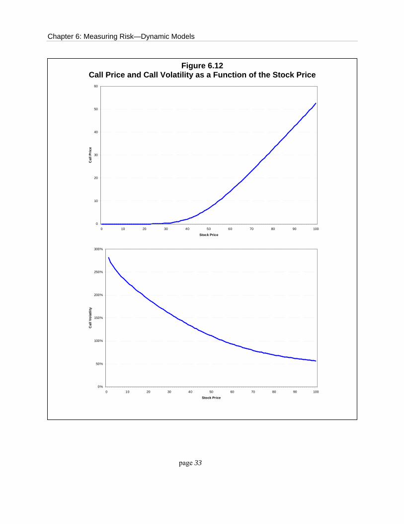
The top panel of Figure 6.12 shows the graph of the call price as a function of the stock

price. For this calculation we have set the exercise price to $50, the maturity to 1 year, the

volatility to 30% and the risk-free interest rate to 5%. The key fact to notice is that the graph is

not linear. Only as the stock goes deep in-the-money, i.e. the stock price is above the exercise

price, does the function become approximately linear. When the stock price is below the exercise

price so that the call option is out-of-the-money, the function is very convex. One consequence of

this relationship is that the riskiness of the call option changes as the stock price changes. We will

write σoption to denote the volatility of the derived option price, and σstock to denote the volatility of

the underlying stock. At very high stock prices, when the option is deep in-the-money, holding

the call is virtually identical to holding the stock, so that the risk of the call option equals the risk

of the stock: σoption ≅ σstock. At very low stock price, when the option is far out-of-the-money, the

risk of the option grows far above the risk of the stock: σoption > σstock.

The formula relating the risk of the option to the risk of the stock is:

S Δ S N (d1 )σoption = σstock × |Ω| = σstock = σstock C C

where Ω is the option elasticity and Δ is the option delta, the measure of the change in the option

price for a $1 change in the stock price. The bottom panel of Figure 6.13 shows the graph of the

volatility of the call price as a function of the stock price. Recall that the volatility of the stock

price is constant, regardless of the level of the stock price. At very high stock prices, the volatility

of the call is almost double the volatility of the stock. As the stock price drops, the volatility of

the call price grows, and grows sharply, so that the volatility of a far out-of-the-money option

grows to nearly ten times the volatility of the stock.

This is a good illustration of how important it is to understand the relationship between

the risk of the underlying factor and the risk of the derivative asset. One underlying factor for a

commodity producer – a gold mining company, for example – is the price at which it can sell the

commodity. If the company will produce the gold regardless of how low the price goes, then its

payoff will be linear with the gold price. Suppose instead that the company has flexibility to

respond to changes in the gold price. Suppose it will shut down some production as the price of

page 20


gold falls, and if the company owns some mines that it will reopen or potential mines that it will

develop should the gold price rise sharply, then the company’s payoff will be non-linear in the

price of gold, and the company’s risk will change as the gold price changes just as the call option

risk changes as the stock price changes.

6.11 Application of the Random Walk to Other Variables

The use of stochastic processes in the field of finance was pioneered through the

development of the geometric Brownian motion model applied to stocks. As the power of this

tool became clear, it also occurred to many analysts that this tool could be applied to modeling

many other variables. Unfortunately, the widespread application of this model to other variables

reflected the adage, “when the only tool you have is a hammer, everything looks like a nail." In

the following section, we will discuss alternative stochastic processes and their application to

modeling appropriately selected variables. Nevertheless, there are some variables where this

simple model has, perhaps, been usefully applied.

One such case is the price of gold. This is because gold is used as an investment vehicle,

and because the cost of storing gold is relatively small. For example, in analyzing the hedging

strategies of gold companies, Fehle and Tysplakov (2005) model the gold price based on data

from 1992-2000 setting the mean annual return at 2% and the annual volatility at 10%.2

d’Halluin et al. (2003) examine how to determine when to expand bandwidth capacity on

a wireless network when the growth in traffic is modeled as a geometric Brownian motion.3

The random walk model is a very specialized process with particular properties that make

it attractive for modeling stock prices. One such feature is the property that the uncertainty about

future stock price grows without bound. There is no maximum beyond which the price is certain

not to go.

A second key feature of this model is that changes in the current spot price translate one-

for-one into a permanent revision of the forecast of future prices. There is no such thing as a

temporary shock to the stock price, i.e., a shock in which the stock price goes up and then

predictably comes down again.

2 Fehle, F. and S. Tysplakov, (2005), Dynamic risk management: Theory and evidence, Journal of Financial Economics 78, 3–47. 3 d’Halluin, Y., P.A. Forsyth, and K.R. Vetzal, 2003, “Wireless Network Capacity Investment,” Working Paper.

page 21


The two panels of Figure 6.13 illustrate this second key feature, the permanent impact of

any shock in a random walk process. The top panel shows a historic sample of data for a price

series. The price has recently experienced a sharp run-up. If we were to forecast the future path of

the price using the random walk model, our forecast would follow the nearly straight line heading

to the right and slightly upward. This line reflects the expected rate of growth in the price, μ. The

forecast takes off from wherever is the most recent value. Any further run-up in the price above

the expected growth rate will shift the whole forecast line up, at all horizons. This is the sense in

which any shock or innovation to the price is treated as a permanent shock.

The bottom panel of Figure 6.13 shows the same historic price data, but constructs a

forecast of future prices by applying a different model, the mean reverting model. The mean is

shown as a dashed line running through the historic data and continuing out into the future time.

The most recent run-up in the historic price series has sent the price far above the mean. In the

mean reverting model, we expect the price to return back to the mean. The forecast is shown as

the curved line heading down from the most recent historic price towards the mean and ultimately

asymptoting to the mean. The mean price is growing at a rate μ, but the actual price is forecasted

to be declining until it returns close enough back to the mean. Therefore, the recent run-up in

price is viewed exclusively as a temporary shock. The long-run forecast is entirely unaffected by

the shock. Only the short-run forecast is dragged upward.

This property of the random walk makes the model very easy to handle. Not only are the

forecasted distributions normal variables, but because of this “permanent shock” property, the

conditional distribution always have the same structure, no matter the current value of the

variable. This makes working with the data and estimating the parameters very simple. There are

never any complicated adjustments to be made. In a mean-reverting model, the conditional

distributions are changing depending upon the current value of the variable. This makes working

with the data and estimating parameters more difficult since adjustments have to be made to

compensate or reflect these changing conditional distributions.

We can illustrate the difference with the simple example of reporting volatility on an

annualized basis. Suppose we measure returns using weekly data and calculate a weekly

volatility. The annualized volatility is calculated by taking the weekly volatility and multiplying

by the square root of 52. This makes sense with the random walk because the volatility grows by

the square root of time, and the volatility in the process never changes. The annualized weekly

volatility should roughly match what you would get if you calculated the volatility from annual

page 22


data. But the same is not true with a mean reverting process. Annualizing the weekly volatility by

multiplying it by the square root of 52 will produce a number that is larger than what you would

get if you calculated the annual volatility from annual data. With a mean reverting process, one

needs to take more care in this type of reporting and comparison.

Unfortunately, the ‘permanent shock’ property is exactly what makes the random walk

model unattractive for representing the dynamics of many other variables that determine project

cash flows and values. These factors include interest rates, foreign exchange rates, various

commodity prices such as oil, natural gas and electricity, and many others. Many of these other

factors exhibit more complicated conditional forecasts. Many exhibit mean reversion of one form

or another, for example. In most cases it is a mistake to casually move from returns and volatility

measured and denominated over one interval of time to returns and volatility measured and

denominated over another interval. So it is necessary to develop other models appropriate to the

peculiar dynamics of these other, underlying factors central to asset valuation and management.

Having already alluded to the properties of a mean reverting process, it is now time to

formally present one. The next part of this chapter develops the pure mean reverting process and

shows how it is used to model interest rates. The final part of the chapter gives a brief overview

of other processes that are used to model a wide range of commodity prices and other factors.

page 23


Figure 6.1 Period Layout for a Monte Carlo Simulation

Δt

t = t0 t1 t2 tN=T=2

time

i = 0 1 2 3 4 5 6 7 8=N

Time horizon, T=2 years, Number of periods in total, N=8,

Number of periods per year, n=N/T=4, Length of a period, Δt=1/n=0.25, i.e., quarterly.

Time horizon, T=2 years,

page 24


page 25

Figure 6.2 Simulations of the Same Horizon Using Different Period Lengths

0

5

10

15

20

0 0.25 0.5 0.75 1

0

5

10

15

20

0 0.25 0.5 0.75 1

period = one week

0

5

10

15

20

0 0.25 0.5 0.75 1

period = one trading day

period = one month


Figure 6.3 Four Sample Paths of the Same Simulation

simulated stock price paths 45

35

25

15

5

0 1 2 3 4 5

simulated cumulative returns 150%

100%

50%

0% 0 1 2 3 4 5

-50%

page 26


Figure 6.4 Histograms for a Sample of 100 Paths

Cumulative Returns to T=2 Years

1 0

4

13

19

23

21

14

4

1 0

0

5

10

15

20

25

-74% -53% -33% -12% 9% 30% 50% 71% 92% 112% Above

cumulative return (labels show top of bin)

freq

uenc

y in

sam

ple

Stock Price at T=2 Years

1

9

18

21

15

11

4 3

1 0 0

0

5

10

15

20

25

47.63 76.56 105.49 134.42 163.36 192.29 221.22 250.15 279.08 308.02 Above

stock price (labels show top of bin)

freq

uenc

y in

sam

ple

page 27


Figure 6.5 Model Probability Distributions

0.000

0.200

0.400

0.600

0.800

1.000

1.200

1.400

-100% -80% -60% -40% -20% 0% 20% 40% 60% 80% 100% 120% 140%

Cumulative Return @ t=2

prob

abili

ty d

ensi

ty

19.2% mean cum return

0.000

0.005

0.010

0.015

0.020

0.025

0.030

0.035

0.040

0 50 100 150 200 250 300 350

Stock Price @ t=2

prob

abili

ty d

ensi

ty

121.12 median price

127.12 mean price

Figure 6.6 Expected Values with Confidence Bounds

-20%

-10%

0%

10%

20%

30%

40%

50%

60%

0.0 0.5 1.0 1.5 2.0

Years

Cum

ulat

ive

Ret

urn

Upper Mean Lower

$0

$20

$40

$60

$80

$100

$120

$140

$160

$180

0.0 0.5 1.0 1.5 2.0

Years

Sto

ck P

rice Upper

Mean Median Lower

page 28


Figure 6.7 One-Step in a Binomial Tree

t=0 t=1

high return, U= high log price= high price, SU=

31.6% 2.618 13.71

initial price, S0= initial log price=

10.00 2.303

low return, D= low log price= low price, SD=

-12.4% 2.178 8.83

page 29


Figure 6.9 Two Steps in a Binomial Tree

t=0 t=1 t=2

return, U= 31.6% cum return UU= 63.2% log price= 2.934 price, SUU= 18.81

high return, U= 31.6% high log price= 2.618 high price, SU= 13.71

return, D= -12.4% cum return UD= 19.2% log price= 2.494 price, SUD= 12.11

initial price, S0= 10.00 initial log price= 2.303

return, U= 31.6% cum return DU= 19.2% log price= 2.494 price, SDU= 12.11

low return, D= -12.4% low log price= 2.178 low price, SD= 8.83

return, D= -12.4% cum retuDD= -24.8% log price= 2.054 price, SDD= 7.80

page 30


Figure 6.10 Recombining in a Binomial Tree

return, U= 31.6% cum return UU= 63.2%

13.71

high return, U= 31.6% log price= 2.934 high log price= 2.618 price, SUU= 18.81 high price, SU=

return, D= -12.4% initial price, S0= 10.00 cum return UD= 19.2% initial log price= 2.303 log price= 2.494

price, SUD= 12.11

-12.4%low return, D= low log price= 2.178 return, D= -12.4%low price, SD= 8.83 cum retuDD= -24.8%

log price= 2.054 price, SDD= 7.80

page 31


Figure 6.11 A 24 Period Recombining Binomial Tree

\ PeriodNode \ 0 1 2 3 4 5 6 7 8 9 10 11 12 13 14 15 16 17 18 19 20 21 22 23 24

0 0.00001% 1 0.00014% 2 0.00165% 3 0.01206% 4 0.06334% 5 0.25334% 6 0.80225% 7 2.06294% 8 4.38375% 9 7.79333%

10 11.69000% 11 14.87818% 12 16.11803% 13 14.87818% 14 11.69000% 15 7.79333% 16 4.38375% 17 2.06294% 18 0.80225% 19 0.25334% 20 0.06334% 21 0.01206% 22 0.00165% 23 0.00014% 24 0.00001%

page 32


Figure 6.12 Call Price and Call Volatility as a Function of the Stock Price

0

10

20

30

40

50

60

0 10 20 30 40 50 60 70 80 90 100

Stock Price

Cal

l Pri

ce

0%

50%

100%

150%

200%

250%

300%

0 10 20 30 40 50 60 70 80 90 100

Stock Price

Cal

l Vol

atlit

y

page 33


Figure 6.13 Forecast Made Using a Random Walk Model

vs. Forecast Made Using a Mean Reverting Model

pric

e pr

ice

time

history RW forecast

time

history mean MR forecast

page 34


Table 6.1 Calculation of a Sample Path

random cumulative stock week variable return return price

0 12.00 1 1.57580 4.99% 4.99% 12.61 2 0.34769 1.24% 6.24% 12.77 3 -2.42436 -7.21% -0.98% 11.88 4 -0.01376 0.14% -0.83% 11.90 5 -0.94792 -2.71% -3.54% 11.58 6 1.72028 5.43% 1.89% 12.23 7 0.14646 0.63% 2.52% 12.31 8 1.39280 4.43% 6.96% 12.86 9 -0.34718 -0.87% 6.08% 12.75

10 -0.98923 -2.83% 3.25% 12.40

page 35


Table 6.2 Estimating Drift and Volatility Parameters

stock week price return

0 12.00 1 12.61 4.99% 2 12.77 1.24% 3 11.88 -7.21% 4 11.90 0.14% 5 11.58 -2.71% 6 12.23 5.43% 7 12.31 0.63% 8 12.86 4.43% 9 12.75 -0.87%

10 12.40 -2.83%

Mean 0.32% Std. Dev. 3.99%

Variable Estimate Input Error μ 21.0% 12.0% 75.2% σ 28.8% 22.0% 30.7%

page 36

Documents

15.997 Practice of Finance: Advanced Corporate Risk Management · 2020-01-04 · 15.997 Practice of Finance: Advanced Corporate Risk Management ... Some students will be familiar