1592 IEEE TRANSACTIONS ON IMAGE PROCESSING, …faculty.ucmerced.edu/mhyang/papers/tip16_reconstructi… · · 2016-04-141592 IEEE TRANSACTIONS ON IMAGE PROCESSING, VOL. 25, NO

1592 IEEE TRANSACTIONS ON IMAGE PROCESSING, VOL. 25, NO. 4, APRIL 2016

Dense and Sparse Reconstruction ErrorBased Saliency Descriptor

Huchuan Lu, Senior Member, IEEE, Xiaohui Li, Lihe Zhang, Xiang Ruan,and Ming-Hsuan Yang, Senior Member, IEEE

Abstract— In this paper, we propose a visual saliency detectionalgorithm from the perspective of reconstruction error. Theimage boundaries are first extracted via superpixels as likelycues for background templates, from which dense and sparseappearance models are constructed. First, we compute dense andsparse reconstruction errors on the background templates foreach image region. Second, the reconstruction errors are propa-gated based on the contexts obtained from K -means clustering.Third, the pixel-level reconstruction error is computed by theintegration of multi-scale reconstruction errors. Both the pixel-level dense and sparse reconstruction errors are then weighted byimage compactness, which could more accurately detect saliency.In addition, we introduce a novel Bayesian integration methodto combine saliency maps, which is applied to integrate thetwo saliency measures based on dense and sparse reconstructionerrors. Experimental results show that the proposed algorithmperforms favorably against 24 state-of-the-art methods in termsof precision, recall, and F-measure on three public standardsalient object detection databases.

Index Terms— Saliency detection, dense/sparse reconstructionerror, sparse representation, context-based propagation, regioncompactness, Bayesian integration.

I. INTRODUCTION

V ISUAL saliency is concerned with the distinct percep-tual quality of biological systems which makes certain

regions of a scene stand out from their neighbors and catchimmediate attention. Numerous biologically plausible modelshave been developed to explain the cognitive process ofhumans and animals [1], [2]. In computer vision, moreemphasis is paid to detect salient objects in images basedon features with generative and discriminative algorithms.Due to its advantage of reducing the complexity of sceneanalysis, saliency detection plays an important preprocessing

Manuscript received May 13, 2015; revised October 1, 2015 andDecember 18, 2015; accepted January 21, 2016. Date of publication Feb-ruary 2, 2016; date of current version February 23, 2016. The work of H. Luand L. Zhang were supported by the National Natural Science Foundationof China under Grant 61528101, Grant 61472060, and Grant 61371157. Theassociate editor coordinating the review of this manuscript and approving itfor publication was Prof. Yongyi Yang.

H. Lu, X. Li, and L. Zhang are with the Faculty of Electronic Informa-tion and Electrical Engineering, School of Information and CommunicationEngineering, Dalian University of Technology, Dalian 116024, China (e-mail:[email protected]; [email protected]; [email protected]).

X. Ruan is with OMRON Corporation, Kusatsu 525-0035, Japan (e-mail:[email protected]).

M.-H. Yang is with the Department of Electrical Engineering and ComputerScience, University of California at Merced, Merced, CA 95344 USA (e-mail:[email protected]).

Color versions of one or more of the figures in this paper are availableonline at http://ieeexplore.ieee.org.

Digital Object Identifier 10.1109/TIP.2016.2524198

role in many computer vision tasks, including image segmen-tation [3], categorization [4], detection [5], recognition [6], [7],thumbnailing [8] and compression [9], [10], to name a few.

Recently many saliency detection approaches have beenproposed, which can be generally divided into two cate-gories: slow, knowledge-driven, top-down models and fast,data-driven, bottom-up models. Contrast-based saliency hasbeen widely investigated in recent years and has become one ofthe most active sub-topics in bottom-up saliency. The researchon contrast-based saliency mainly focuses on two aspects,which can be summarized as “how to contrast” and “whatto contrast with”.

Motivated by the neuronal architecture of the earlyprimate vision system, Itti et al. [11] propose a saliencydetection model based on multi-scale image features anddefine visual attention as the local center-surround differ-ence, which is the early answer to “what to contrast with.”Klein and Frintrop [12] regard the center-surround differenceas the multi-scale contrast of the center and surround featuredistributions, inspired by the information theory Kullback-Leibler divergence. While center-surround contrast-based mea-sures are able to detect salient objects, existing bottom-upapproaches are less effective in suppressing background pixels.Different from the center-surround contrast, local contrast ismeasured by comparing a region only with its relevant contexts(defined as a set of region neighbors in the spatial or featurespace) [13]–[15].

Despite local contrast accords with the neuroscience princi-ple global contrast should also be taken into account when oneregion is similar to its surrounds but still distinct in the wholescene. In other words, global contrast aims to capture theholistic rarity or uniqueness from an image. Achanta et al. [16]use global Gaussian blur to suppress noise and high frequencypatterns but do not account for spatial relationship, which maylead to highlighted background. Recent methods [17], [18]measure global contrast-based saliency based on spatiallyweighted feature dissimilarities. Perazzi et al. [19] formulatesaliency estimation using two Gaussian filters by which colorand position are respectively exploited to measure regionuniqueness and distribution.

Recent years, saliency detection algorithms based on learn-ing [20], [21] or deep learning [22], [23] techniques haveattracted more and more attention. Lu et al. [20] first learnoptimal saliency seeds, and then propagates saliency informa-tion under a diffusion framework. Liu et al. [21] learn a novelPartial Differential Equation system adaptively to model the

1057-7149 © 2016 IEEE. Personal use is permitted, but republication/redistribution requires IEEE permission.See http://www.ieee.org/publications_standards/publications/rights/index.html for more information.

LU et al.: DENSE AND SPARSE RECONSTRUCTION ERROR-BASED SALIENCY DESCRIPTOR 1593

Fig. 1. Saliency maps based on dense and sparse reconstructionerrors. Brighter pixels indicate higher saliency values. (a) Original images.(b) (c) Saliency maps from dense and sparse reconstruction, respectively.(d) The Bayesian integrated saliency map of (b) and (c). (e) Ground truth.

learned saliency seeds propagation process. Zhao et al. [22]employ deep Convolutional Neural Networks (CNNs) forvisual saliency detection which simultaneously take global andlocal context into consideration. In [23], multi-scale featuresare extracted by CNNs to model a high-quality saliencydetection framework.

In this paper, we exploit image boundaries as the likelybackground regions from which templates are extracted.Motivated by the observations that dense representation frombackground template is able to capture the intrinsic propertiesof background characteristic but is sensitive to noise, whilesparse representation manages to model the uniqueness andcompactness of regions but is less robust when backgroundtemplates incorporate foreground regions, we use their com-bination as indication of saliency which will work in acomplementary way to compensate for the defects of eachother. We exploit a context-based propagation mechanism toobtain more uniform reconstruction errors over the image.The reconstruction error of each pixel is then assigned by anintegration of multi-scale reconstruction errors. Furthermore,we incorporate region compactness into the dense andsparse reconstruction errors to further improve their accuracy.In addition, we present an effective Bayesian integrationmethod to combine saliency maps constructed from dense andsparse reconstruction (see Figure 1).

The main contributions of this work are as follows:1. We propose an algorithm to detect salient objects by denseand sparse reconstruction for each individual image, whichcomputes more effective bottom-up contrast-based saliency.2. A context-based propagation mechanism is proposed forregion-based saliency detection, which uniformly highlightsthe salient objects and smooths the region saliency.3. A compactness weighted reconstruction error is proposedby incorporating spatial compactness into the dense and sparsereconstruction errors.4. We present a Bayesian integration method to combinesaliency maps, which achieves more favorable results than theexisting integration strategy.

II. RELATED WORKS

A. Boundary Prior for Saliency Detection

According to the basic rule of photographic compositionthat human photographers tend to place objects of interest inthe center of photographs [24], Wei et al. [25] define geodesicsaliency by regarding image boundaries as background priors,

which is validated reasonable and effective. Based on the factthat there is a strong center bias in some saliency detectiondatabases [26], we also consider image boundary regions asbackground priors for saliency detection. However differentfrom [25], we extract image boundary regions as likely cuesfor background templates, by which dense and sparse recon-struction errors are computed for each image region.

B. Image Representation for Saliency Detection

To describe patch features in a relatively low dimensionalspace, Duan et al. [18] adopt an equivalent method to Prin-ciple Component Analysis (PCA) to reduce data dimensionand use the reduced dimensional feature to calculate patchdissimilarities. Sparse representation is similarly employed asa way of image feature representation in [15], [27], and [28],with a dictionary trained from a large set of natural imagefeatures. Since each image patch is represented by a dictionaryor basis functions learned from a set of natural image patchesrather than the remaining other patches of its correspondingimage, the most relevant visual information of each individualimage is not fully extracted and exhaustively used in saliencyestimation. Therefore, these methods do not uniformly detectsalient objects or suppress the background in a scene.

To address the above mentioned issues, we make full useof image visual information by constructing background basesfrom the extracted background templates for each individualimage. From the view of reconstruction, we assume thatthe image background can be better reconstructed than theforeground by a linear combination of the background bases.Therefore, the contrast-based saliency of an image regionis indicated by its reconstruction error, which implies itsdifference from the background information. In other words,larger reconstruction error based on the background templatesindicates larger saliency value for an image region.

C. Bayesian Inference for Saliency Detection

Bayes formula is used in many saliency detection modelssuch as [24], [29], and [30]. Zhang et al. [24] propose asaliency detection algorithm based on a Bayesian frameworkfrom which bottom-up saliency emerges naturally as the self-information of visual features. Xie and Lu [30] develop aprior map to replace the constant value in [29] as Bayesprior probability, which largely improves the accuracy ofBayes posterior probability. Both [29] and [30] compute thelikelihood probability through CIELab color. However, thenoise in color space may be introduced again despite it hasbeen removed by the prior, which may have negative impacton the posterior, sometimes even make the posterior moreinaccurate than the prior. Therefore, if a saliency map whichbetter expresses image saliency than color information acts asthe observation likelihood, a more accurate Bayes posteriorprobability could be achieved, as done in this work.

III. DENSE AND SPARSE RECONSTRUCTION ERRORS

We use both dense and sparse reconstruction errors tomeasure the saliency of each image region. We note that


Fig. 2. Main steps of dense and sparse reconstruction errors.

a dense appearance model renders more expressive andgeneric descriptions of background templates, whereas asparse appearance model generates unique and compactrepresentations. It is well known that dense appearancemodels are more sensitive to noise. For cluttered scenes, denseappearance models may be less effective in measuring salientobjects via reconstruction errors. On the other hand, solutions(i.e., coefficients) by sparse representation are less stable(e.g., similar regions may have different sparse coefficients),which may lead to discontinuous saliency detection results.In this work, we use both representations to model regionsand measure saliency based on reconstruction errors.

The dense and sparse reconstruction errors are obtainedas shown in Figure 2. First, we extract the image boundarysegments as the background templates for saliency detection.Second, we reconstruct all the image regions based on thebackground templates and normalize the reconstruction errorsto the range of [0, 1]. Third, a propagation mechanism isproposed to exploit local contexts obtained from K-meansclustering. Forth, pixel-level reconstruction error is computedby integrating multi-scale reconstruction errors.

A. Background Templates

To better capture structural information, we first generatesuperpixels using the simple linear iterative clustering (SLIC)algorithm [31] to segment an input image into multiple uni-form and compact regions (i.e., segments). We use the meanLab and RGB color features and coordinates of pixels todescribe each segment by x = {L, a, b, R, G, B, x, y}�. Theentire image is then represented as X = [x1, x2, . . . , xN ] ∈R

D×N , where N is the number of segments and D is thefeature dimension. Motivated by the representation ability ofimage boundary, we extract the D-dimensional feature of eachboundary segment as b and construct the background templateset as B = [b1, b2, . . . , bM ], where M is the number ofimage boundary segments Figure 2 shows some backgroundtemplates extracted at different scales. Given the backgroundtemplates, we compute two reconstruction errors by dense andsparse representation for each image region, respectively.

B. Dense Reconstruction Error

A segment with larger reconstruction error based on thebackground templates is more likely to be the foreground.Based on this concern, the reconstruction error of each region

Fig. 3. Saliency maps based on dense and sparse reconstructionerrors. Brighter pixels indicate higher saliency values. (a) Original images.(b) Saliency maps from dense reconstruction. (c) Saliency maps from sparsereconstruction. (d) Ground truth.

is computed based on the dense appearance model gener-ated from the background templates B = [b1, b2, . . . , bM ],B ∈ R

D×M using Principal Component Analysis (PCA).The eigenvectors from the normalized covariance matrix

of B, UB = [u1, u2, . . . , uD′ ], corresponding to the largestD′ eigenvalues, are computed to form the PCA bases of thebackground templates. With the PCA bases UB, we computethe reconstruction coefficient of segment i (i ∈ [1, N]).

βi = UB�(xi − x̄), (1)

and the dense reconstruction error of segment i is

εdi = ‖xi − (UBβi + x̄)‖2

2 , (2)

where x̄ is the mean feature of X. The saliency measure isproportional to the normalized reconstruction error (within therange of [0, 1]).

Figure 3(b) shows some saliency detection results via densereconstruction. Dense representations model data points witha multivariate Gaussian distribution in the feature space,and thus it may be difficult to capture multiple scatteredpatterns especially when the number of examples is limited.Therefore, when image saliency detection encounters compli-cated background, it may be difficult for the dense appearancemodel to train a set of background bases which could extractcomplete background information, thus leading to backgroundnoise in saliency map. The first row of Figure 3 shows anexample where some background regions have large densereconstruction errors (i.e., inaccurate saliency measure).

C. Sparse Reconstruction Error

Motivated by the demonstrated success of sparsity-basedclassifiers for computer vision tasks [32], [33], we make an


assumption that the background can be better represented thanthe foreground by a linear combination of the backgroundtemplates. We use the set of background templates B asthe bases for sparse representation, and encode the imagesegment i by

α∗i = argmin

αi

‖xi − Bαi‖22 + λ‖αi‖1, (3)

and the sparse reconstruction error is

εsi = ∥

∥xi − Bα∗i

∥∥2

2 . (4)

Since all the background templates are regarded as the basisfunctions, sparse reconstruction error can better suppressthe background compared with dense reconstruction errorespecially in cluttered images, as shown in the middle rowof Figure 3.

Nevertheless, there are some drawbacks in measuringsaliency with sparse reconstruction errors. If some fore-ground segments are collected into the background templates(e.g., when objects appear at the image boundaries), theirsaliency measures are close to 0 due to low sparse recon-struction errors. In addition, the saliency measures for theother regions are less accurate due to inaccurate inclusionof foreground segments as part of sparse basis functions.On the other hand, the dense appearance model is not affectedby this problem. When foreground segments are mistakenlyincluded in the background templates, the extracted principlecomponents from the dense appearance model may be lesseffective in describing these foreground regions. As shown inthe second row of Figure 3, when some foreground segmentsat the image boundary (e.g., torso and arm) are not detectedvia sparse reconstruction, these regions are still be detected bythe dense counterpart.

We note sparse reconstruction error is more robust to dealwith complicated background, while dense reconstruction erroris more accurate to handle the object segments at imageboundaries. Therefore, dense and sparse reconstruction errorsare complementary in measuring saliency.

D. Context-Based Reconstruction Error Propagation

Considering that even the best segmentation algorithmscan not avoid to separate an image region into multiplesmaller homogeneous ones. Thus two segments sharing similarfeatures in the feature space may share different reconstructionerrors, which results in discontinuous saliency maps. On theother hand, even though salient objects do not touch the imageboundaries in most cases, some background templates maybe part of foreground in fact. In this case, the reconstructionerrors may not precisely represent the contrast with the truebackground and consequently results in mistakes in saliencydetection.

To overcome the above two problems, we propose a context-based error propagation method to smooth the reconstructionerrors generated by dense and sparse appearance models.Both dense and sparse reconstruction errors of segment i(i.e., εd

i and εsi ) are denoted by εi for conciseness.

We first apply the K-means algorithm to cluster N imagesegments into K clusters via their D-dimensional features and

Fig. 4. Saliency maps with the context-based error propagation. (a) and (b)are original images and ground truth. (c) and (d) are original and propagateddense reconstruction errors. (e) and (f) are original and propagated sparsereconstruction errors.

initialize the propagated reconstruction error of segment i asε̃i = εi . All the segments are sorted in descending orderby their reconstruction errors and considered as multiplehypotheses. They are processed sequentially by propagatingthe reconstruction errors in each cluster. The propagatedreconstruction error of segment i belonging to cluster k(k = 1, 2, . . . , K ), is modified by considering its appearance-based context consisting of the other segments in cluster k asfollows:

ε̃i = τ

Nc∑

j=1

wik j ε̃k j + (1 − τ ) εi , (5)

wik j =exp(−

∥∥∥xi−xk j

∥∥∥

2

2σx2 )(

1 − δ(

k j − i))

Nc∑

j=1exp(−

∥∥∥xi −xk j

∥∥∥

2

2σx2 )

, (6)

where {k1, k2, . . . , kNc } denote the Nc segment labels in clusterk and τ is a weight parameter. The first term on the righthandside of Eq. 5 is the weighted averaging reconstruction error ofthe other segments in the same cluster, and the second termis the initial dense or sparse reconstruction error. That is, forsegment i , by considering all the other segments belonging tothe same cluster k (i.e., the appearance-based local context),the reconstruction error can be better estimated. The weight ofeach segment context is defined by its normalized similaritywith segment i in Eq. 6, where σ 2

x is the sum of the variance ineach feature dimension of X and δ(·) is the indicator function.

Figure 4 shows two examples where the context-basedpropagation mechanism smooths the reconstruction errors ina cluster, thereby uniformly highlighting the image objects.The bottom row of Figure 4 presents one case that severalsegments of the object (e.g., torso) are mistakenly includedin the background templates, and therefore they are not cor-rectly identified by the dense and sparse appearance models.Nevertheless, the reconstruction errors of these segments aremodified by taking the contributions of their contexts intoconsideration using Eq. 5.

E. Pixel-Level Reconstruction Error

For a full-resolution saliency map, we assign saliency toeach pixel by integrating results from multi-scale reconstruc-tion errors.

To handle the scale problem, we generate superpixels atNs different scales. We compute and propagate both dense


Fig. 5. Saliency maps with the multi-scale integration of propagatedreconstruction errors. (a) and (b) are original images and ground truth.(c) and (d) are propagated dense reconstruction errors without and withintegration. (e) and (f) are propagated sparse reconstruction errors withoutand with integration.

and sparse reconstruction errors for each scale. We integratemulti-scale reconstruction errors and compute the pixel-levelreconstruction error by

E(z) =

Ns∑

s=1ωzn(s) ε̃n(s)

Ns∑

s=1ωzn(s)

, ωzn(s) = 1∥∥dz − xn(s)

∥∥

2

, (7)

where dz is a D-dimensional feature of pixel z and n(s)

denotes the label of the segment containing pixel z at scale s.Similarly to [14], we utilize the similarity between pixel zand its corresponding segment n(s) as the weight to averagethe multi-scale reconstruction errors.

Figure 5 shows some examples where objects are moreprecisely identified by the reconstruction errors with multi-scale integration, which suggests the effectiveness of usingmulti-scale integration mechanism to measure saliency.

IV. COMPACTNESS WEIGHTED

RECONSTRUCTION ERROR

Considering that salient regions generally group compactlyin the spatial domain, while background ones always distributeover the entire image with higher spatial variance, we concludethat region compactness in the image spatial domain is vitalto saliency detection.

The dense and sparse reconstruction errors introducedin Section III imply the feature distance of an image region tothe background templates in the color space, which exhibitspromising performance in suppressing the background noise.However, spatially adjacent regions may still share largelydifferent reconstruction errors without considering the colorcompactness or distribution in spatial domain. Therefore wepropose a compactness weighted reconstruction error to mea-sure saliency by taking the color distribution into considerationin order to smooth the object saliency.

A. Region Compactness

Based on the observation that salient regions tend todistribute compactly, we define the region compactness by itsinverse spatial variance, i.e. the smaller the spatial variance is,the larger the compactness is, thus the more salient the regionwill be.

We represent the image segment i as xi = [fi ; pi ] wheref = {L, a, b, R, G, B}� and p = {x, y}� denote the color

Fig. 6. Saliency maps based on compactness weighted reconstructionerror. (a) Original images. (b) Saliency maps from sparse reconstruction.(c) Saliency maps generated by region compactness. (d) Saliency maps basedon compactness weighted reconstruction error. (e) Ground truth.

feature and position information of each segment respectively.Then the region compactness of segment i can be defined as

ci = 1 − ||N∑

j=1

πi j p j2 − (

N∑

j=1

πi j p j )2||1, (8)

where

πi j =exp(−‖fi −f j‖

2σf2

2)

N∑

j=1exp(−‖fi−f j‖

2σf2

2)

. (9)

The squared position is computed as p2 = {x2, y2}� in Eq. 8.The region position is weighted by the normalized colorsimilarity in Eq. 9 similarly to [19], where σ 2

f is the sumof the variance in each feature dimension similarly to σ 2

xin Eq. 6. The color weighted region position minus themean weighted region position effectively describes the spatialdistribution of region i , and L1-norm combines the horizontaland vertical variances together. As summarized in Eq. 8, weinverse the description of the spatial distribution to calculateregion compactness over the entire image.

Figure 6(c) shows some saliency maps generated by theregion compactness. Compared to the sparse reconstructionerror (Figure 6(b)), the region compactness could highlightthe salient object more uniformly due to the spatially compactdistribution of object color. However, the region compact-ness is more sensitive to background noise. The bottom rowof Figure 6 shows a failure case where the object is of largesize and the background color is uniformly distributed, whichconsequently leads to false object detection. Therefore wepropose a compactness weighted reconstruction error in orderto further enhance the contrast between salient object andbackground.

B. Compactness Weighted Reconstruction Error

Without taking region compactness into consideration, thereconstruction error of salient object is not grouped as well asthe color feature. Therefore we weigh the reconstruction errorintroduced in Section III by the region compactness.


We first propagate the initial region compactness (i.e., ci foreach segment in Eq. 8) and integrate the multi-scale results toobtain pixel-level compactness as C(z) for pixel z, similarlyto the reconstruction error E(z) in Eq. 7. Then we calculatethe compactness weighted reconstruction error for pixel z as

E(z) = wC (z) ∗ E(z), (10)

where function wC (·) can be any positive weight function(e.g., exponential, log and sigmoid function) of region com-pactness and we simply define it as wC (z) = C(z) inthis work.

Figure 6 shows three examples where the compactnessweighted sparse reconstruction error performs better than thenon-weighted one. As shown on the top and middle row, thesalient object uniformly pops out due to the region compact-ness which presents larger contrast between the foreground andbackground than the reconstruction error. However, we notethat region compactness may be more sensitive to the back-ground noise than the reconstruction error (see the bottom tworows of Figure 6). By taking spatial distribution into account,the compactness weighted reconstruction error could reducethe negative impact of region compactness and highlight theforeground as well as suppress the background. The weightedreconstruction error detects the salient regions more accuratelyand uniformly, even correcting the false detection by the regioncompactness in the bottom image. In summary, as an importantfactor for saliency detection, the region compactness largelyhelps to locate the object by weighing the reconstruction error.

C. Saliency Assignment Refined by Object-Biased Gaussian

Borji et al. show that there is a center bias in some saliencydetection datasets [26]. Recently center prior has been usedin [14], [15], [18], [19], and [34] and usually formulated as aGaussian model,

G (z) = exp

[

−(

(xz − μx )2

2σx2 +

(

yz − μy)2

2σy2

)]

, (11)

where μx = xc and μy = yc denote the coordinates of theimage center and xz and yz are the coordinates of pixel z.Since salient objects do not always appear at the image centeras Figure 7 shows, the center-biased Gaussian model is noteffective and may include background pixels or miss theforeground regions. We use an object-biased Gaussian modelGo with μx = xo and μy = yo, where xo and yo denote theobject center derived from the pixel error in Eq. 7:

xo =∑

i

E(i)∑

jE( j)

xi , yo =∑

i

E(i)∑

jE( j)

yi . (12)

We set σx = 0.25 × H and σy = 0.25 × W , where W and Hrespectively denote the width and height of an image. Withthe object-biased Gaussian model, the saliency of pixel z iscomputed by

S (z) = Go (z) ∗ E (z). (13)

Figure 7 shows an example when the object does not locateat the image center. Comparing the two refined maps of the

Fig. 7. Comparison of center-biased (Gc) and object-biased (Go) Gaussianrefinement. Ed and Es are the multi-scale integrated dense and sparsereconstruction error maps, respectively.

saliency via dense or sparse reconstruction in the bottom row,the proposed object-biased Gaussian model renders moreaccurate object center, and therefore better refines the saliencydetection results.

V. BAYESIAN INTEGRATION OF SALIENCY MAPS

As mentioned in Section III, the saliency measures bydense and sparse reconstruction errors are complementaryto each other. To integrate both the saliency measures, wepropose an integration method by Bayesian inference, differentfrom the conventional integration strategy simply by weightedaveraging saliency maps in [25] and [26].

A. Bayes Formula

Recently, the Bayes formula has been used to measuresaliency by the posterior probability in [29] and [35]:

p(F |H (z)) = p(F)p(H (z)|F)

p(F)p(H (z)|F) + (1 − p(F))p(H (z)|B),

(14)

where the prior probability p(F) is a uniform [29] or asaliency map [35] and H (z) is a feature vector of pixel z.The observation likelihood probabilities are computed as:

p(H (z)|F) =∏

r∈{L ,a,b}

NbF (r(z))

NF,

p(H (z)|B) =∏

r∈{L ,a,b}

NbB (r(z))

NB, (15)

where NF denotes the number of pixels in the foregroundand NbF (r(z))(r ∈ {L, a, b}) is the number of pixels whosecolor features fall into the foreground bin bF (r(z)) whichcontains feature r(z), while the color distribution histogramof the background is denoted likewise by NB and NbB (r(z)).However, the noise in color space may be introduced again


Fig. 8. Bayesian integration of saliency maps. The two saliency measuresvia dense and sparse reconstruction are respectively denoted by S1 and S2.

though it has been removed by the prior probability, and resultsin inaccurate posterior probability, which makes the posterioreven worse than the prior in some cases.

Considering this problem, we take one saliency map in thiswork as the prior and use the other one instead of Lab colorinformation to compute the likelihoods, which integrates morediverse information from different saliency maps.

B. Bayesian Integration Formula

Given two saliency maps S1 and S2 (i.e., from dense andsparse reconstruction), we treat one of them as the priorSi (i = {1, 2}) and use the other one Sj ( j �= i, j = {1, 2})to compute the likelihood, as shown in Figure 8. First, wethreshold the map Si by its mean saliency value and obtain itsforeground and background regions described by Fi and Bi ,respectively. In each region, we compute the likelihoodsby comparing Sj and Si in terms of the foreground andbackground bins at pixel z:

p(Sj (z)|Fi ) = NbFi (S j (z))

NFi

, p(Sj (z)|Bi) = NbBi (S j (z))

NBi

. (16)

Consequently the posterior probability is computed with Si

as the prior by

p(Fi |Sj (z)) = Si (z)p(Sj (z)|Fi )

Si (z)p(Sj (z)|Fi ) + (1 − Si (z))p(Sj (z)|Bi ).

(17)

Similarly, the posterior saliency with Sj as the prior is com-puted. We use these two posterior probabilities to compute anintegrated saliency map, SB(S1(z), S2(z)), based on Bayesianintegration:

SB(S1(z), S2(z)) = p(F1|S2(z)) + p(F2|S1(z)). (18)

The proposed Bayesian integration of saliency maps is illus-trated in Figure 8. It should be noted that Bayesian integrationenforces these two maps to serve as the prior and cooperatewith each other in an effective manner, which uniformlyhighlights salient objects in an image. The proposed saliencydetection algorithm via dense and sparse reconstruction issummarized in Algorithm 1.

Algorithm 1 Saliency Detection via Dense and SparseReconstruction

VI. EXPERIMENTS

We evaluate the proposed algorithm with twenty-fourstate-of-the-art algorithms including IT [11], MZ [36],LC [37], GB [38], SR [39], AC [40], FT [16], CA [13],RA [29], RC [17], CB [14], SVO [41], DW [18], SDS [42],SF [19], LR [34], GS [25], XL [35], SIA [43], HS [44],wCO [45], HCT [46], MKB [47], and DSR1 [48] onthree benchmark data sets: ASD, MSRA and SOD.

A. Data Sets

The MSRA database [49] contains 5000 images. The ASDdatabase [16] includes 1000 images selected from the MSRAdatabase. Most images in the MSRA and ASD databaseshave only one salient object and there are usually strongcontrast between objects and backgrounds. In addition, weevaluate the proposed algorithm on the SOD database. TheSOD database [50] is based on the Berkeley segmentationdataset which is more challenging than the other databaseswith multiple objects of different sizes and locations in morecomplicated backgrounds. All images in these dataset corre-spond to manually labeled ground truth. In order to evaluatethe effectiveness of saliency detection models, we employ thecommon used Precision-Recall (PR) curve and F-measure.

B. Parameter Setting

The two main parameters of our method are the numberof clusters K and the weight factor τ in Eq. 5. We setK = 8 and τ = 0.5 in all experiments. The parameter λ ofEq. 3, is empirically set to 0.01. For dense reconstruction, weuse the eigenvectors corresponding to the biggest eigenvalueswhich retain 95% of the energy. For background templateupdate, we empirically set the maximal iteration number to3 in our experiment. For multi-scale reconstruction errors, wegenerate superpixels at eight different scales respectively with50 to 400 superpixels. The developed MATLAB code will bemade available to the public.


Fig. 9. Evaluation of saliency via reconstruction error. (a) Based onthe context-based propagation. (b) Based on the multi-scale reconstructionerror integration. DE: dense reconstruction error; DEP: propagated DE;MDEP: multi-scale integrated DEP; SE: sparse reconstruction error;SEP: propagated SE; MSEP: multi-scale integrated SEP; RC11: baselinemethod [17].

C. Evaluation of Reconstruction Error

We evaluate the proposed dense and sparse reconstructionerrors as well as the compactness weighted ones on theASD database.

1) Reconstruction Error: We evaluate the contribution ofthe context-based propagation and multi-scale reconstruc-tion error integration in Figure 9. The approach in [17](referred as RC11) is also presented as a baseline model forcomparisons. Figure 9(a) shows that the sparse reconstructionerror based on background templates achieves better accuracyin detecting salient objects than RC11 [17], while the denseone is comparable with it. This is due to the strong capacityof dense and sparse reconstruction techniques to model back-ground appearance characters. The context-based reconstruc-tion error propagation method uses segment contexts throughK-means clustering to smooth the reconstruction errors andminimize the detection mistakes introduced by the objectsegments in background templates with improved performance(Figure 9(a)). The reconstruction error of a pixel is assignedby integrating the multi-scale reconstruction errors, whichhelps generate more accurate and uniform saliency maps.Figure 9(b) shows the improved performance due to theintegration of multi-scale reconstruction errors.

2) Compactness Weighted Reconstruction Error: To evalu-ate the compactness weighted reconstruction error, we calcu-late pixel-level compactness by the context-based propagationand multi-scale integration and directly utilize it to describeimage saliency. We quantitatively compare the performanceof the non-weighted and weighted reconstruction errors tofigure out the contribution of region compactness to saliencydetection. We can see from Figure 10(a) that the pixel-levelcompactness shows higher precision than RC11 [17], whichdemonstrates that color compactness is of as much importanceas color uniqueness that used in RC11 [17]. Owing to theincorporated compactness factor, the weighted reconstructionerror achieves better performance in detecting saliency thanthe non-weighted one as shown in Figure 10(a). In addition,we also evaluate the object-biased Gaussian refinement forthe weighted reconstruction error. Figure 10(b) shows that theobject-biased Gaussian model further refines the results andperforms better than the center-biased one.

Fig. 10. Evaluation of saliency via compactness weighted reconstruc-tion error. (a) Based on the compactness weighted reconstruction error.(b) Based on the object-biased Gaussian refinement. Compactness: pixel-levelcompactness; CDE and CSE: compactness weighted dense and sparse recon-struction error; NDE and NSE: non-weighted dense and sparse reconstructionerror; CDEG and CSEG: Gaussian refined CDE and CSE; RC11: baselinemodel [17].

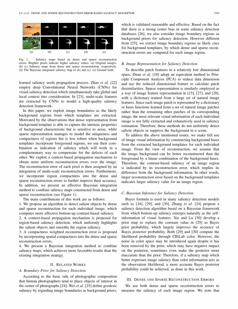
Fig. 11. Saliency maps based on different Bayes posterior probabilities.(a) and (d) are original image and ground truth. (b) and (c) are saliencymaps from Bayes posterior probability. We treat the saliency map by dense(or sparse) reconstruction as the prior, and use the other saliency map bysparse (or dense) reconstruction and Lab color to compute the likelihood,denoted by Dense-Sparse (or Sparse-Dense) and Dense-Lab (or Sparse-Lab),respectively.

D. Evaluation of Bayesian Integration

We also evaluate the proposed Bayesian integration methodfor combining saliency maps.

1) Bayesian Integration of the Dense and Sparse SaliencyMaps: In Section V, we discuss that the posterior probabilitycan be more accurate with likelihood computed by a saliencymap rather than the CIELab color space on the condition ofthe same prior in the Bayes formula. We present experimentalresults in which we treat the saliency map by dense (or sparse)reconstruction as the prior, and use the other saliency map bysparse (or dense) reconstruction and Lab color to computethe likelihood probability, denoted respectively by Dense-Sparse (or Sparse-Dense) and Dense-Lab (or Sparse-Lab)in Figure 11. With the saliency generated by dense (or sparse)reconstruction as the prior, the result with the likelihood basedon sparse (or dense) reconstruction (Figure 11(c)) is moreaccurate than that with the CIELab color space (Figure 11(b)),which suggests that the Bayes posterior probability withlikelihood computed by a saliency map can achieve higherrecall (see the top row) and precision (see the bottom row)than that computed by color information, due to the less noisein the saliency map than CIELab color.


Fig. 12. (a) F-measure curves of the proposed Bayesian integrated saliency and four other integrated ones of CDEG and CSEG. (b) Precision-recall curvesof Bayesian integrated saliency of four state-of-the-art methods. (c) F-measure curves of the proposed Bayesian integrated saliency and four other integratedones of SF [19] and GS [25]. (d) Further improvement of seven state-of-the-art methods by the proposed saliency propagation, where dashed lines areprecision-recall curves of the original state-of-the-art methods, while solid ones are the variants (i.e., the propagated results) denoted by the original namessuffixed with -Prop.

Fig. 13. Saliency maps based on the proposed Bayesian integration.(a) Original images. (d) The Bayesian integrated saliency map of (b) and (c).(e) Ground truth. Sd and Ss are saliency maps via dense and sparsereconstruction, respectively. RC [17], SVO [41], CB [14] and GS [25] denotefour state-of-the-art saliency maps.

In addition, we also present the F-measure curve depictedby the mean F-measure at each threshold from 0 to 255in Figure 12(a). We evaluate the performance of Bayesian inte-grated saliency map SB by comparing it with the integrationstrategies formulated in [26]:

Sc = 1

Z

∑

i

Q (Si ) or Sc = 1

Z

∏

i

Q (Si ), (19)

where Z is the partition function. In Figure 12(a), we denotethe linear summation Sc with Q(x) = {x, exp(x),−1/ log(x)}respectively by Identity, Exp and Log, while denote the accu-mulation Sc with Q(x) = x by Mult. Figure 12(a) shows thatthe F-measure of the proposed Bayesian integrated saliencymap is higher than the other methods at most thresholds, whichdemonstrates the effectiveness of Bayesian integration.

2) Bayesian Integration of State-of-the-Art Saliency Maps:To further validate the effectiveness of the proposed Bayesianintegration mechanism, we implement it on the state-of-the-art methods and evaluate the performance of the integratedsaliency maps. We employ Bayesian integration to combineseveral best salient object detection models reported by [26],including CB [14], SVO [41], RC [17], SF [19] and GS [25].Figure 12(b) shows that the Bayesian integrated saliencyresults SB(RC, SV O) and SB(C B, GS) achieve betterprecision-recall curves than either individual saliency. TheBayesian integrated saliency maps (Figure 13(d)) have com-parable capability to suppress the background with both thetwo individual saliency maps (Figure 13(b) and (c)), andsimultaneously highlight the salient object more uniformly

than them. Due to the uniformly highlighted salient object, therecall value of the integrated saliency map is largely improved,which can be figured out from the quantitative comparisons(see Figure 12(b)) where the minimum recall value of theBayesian integrated saliency is much higher than others.

We also implement the Bayesian integration on SF [19]and GS [25], and compare the integrated result SB(SF, GS)with those obtained by other four conventional integrationformulas (Eq. 19). Figure 12(c) presents the F-measure curvesof the integrated results of SF and GS, including Identity,Mult, Exp, Log, and SB(SF, GS). As shown in Figure 12(c),the Bayesian integrated result SB(SF, GS) achieves higherF-measure than other integrated ones at most thresholds, whichfurther demonstrates the effectiveness of Bayesian integration.

E. Comparisons With State-of-the-Art Methods

We present the evaluation results of the proposed algorithmcompared with the state-of-the-art saliency detection methodson the ASD database in Figure 14, and the MSRA andSOD databases in Figure 15. The precision-recall curvesshow the proposed algorithm achieves consistent and favor-able performance against the state-of-the-art methods. In thebar graphs, the precision, recall and F-measure of theproposed algorithm are comparable with those of the othermethods, especially with higher recall and F-measure value.Figure 16 shows that the proposed model generates moreaccurate saliency maps with uniformly highlighted foregroundand well suppressed background on the ASD, MSRA andSOD databases.

Compared with the latest and best salient object detectionmodels (e.g., HS [44], wCO [45], HCT [46] and MKB [47]),our method achieves better or comparable performanceamong the three databases as shown in Figure 14 and 15.Due to the robust dense and sparse reconstruction model,our saliency map shows better performance than GS [25]which also exploits image boundaries as background priors.wCO [45] introduces the concept of boundary connectivitywhich describes the likelihood of a region belonging to back-ground effectively. Figure 14 and 15 demonstrate that ourbackground templates based reconstruction error acquire simi-lar performance with this approach. HCT [46] combine feature


Fig. 14. Performance of the proposed method compared with twenty-four state-of-the-art methods on the ASD database.

Fig. 15. Performance of the proposed algorithm compared with other state-of-the-art methods on the MSRA and SOD databases, respectively.(a) MSRA. (b) SOD.

Fig. 16. Comparisons of saliency maps. Top, middle and bottom two rows are images from the ASD, SOD and MSRA data sets, respectively.DSR: the proposed algorithm based on dense and sparse reconstruction. DSR cut: cut map using the generated saliency map. GT: ground truth.

TABLE I

COMPARISON OF AVERAGE RUN TIME (SECONDS PER IMAGE)

vectors in high-dimensional color space linearly to distinct thesalient object and background of the input image. However,this algorithm is sensitive to the initial color seed and thehigh-dimensional color transformation does not fully accordwith human visual perception. Therefore, the robustness ofthis framework is undesirable. MKB [47] learns a multi-kernel boost Support Vector Machine (SVM) classifier withina single image. Because of the lack of samples, MKB [47]performs less robust than our proposed algorithm. The pro-posed algorithm DSR2 in this paper also performs better than

the published conference version DSR1 [48] on the ASDand MSRA databases, and achieves comparable experimentalresults on the challenging SOD database.

Run Time: The average run time of the proposed methodand currently top-performance methods on the SOD databaseare presented in Table I based on a machine with Intel(R)Core(TM) i7-3770 3.4GHz CPU and 32GB RAM. Basedon the current implementation without code optimization,the proposed algorithm takes about 5 seconds to process animage (where the most time-consuming part is the multi-scale


superpixel segmentation), which costs less time than thestate-of-the-art salient object detection models (e.g., RA [29],CA [13], LR [34] and SVO [41]).

F. Further Improvement of State-of-the-Art Saliency Maps

As discussed in Section VI-C, the propagated reconstruc-tion error is more accurate than the non-propagated one(see Figure 9(a)), which validates the effectiveness of thecontext-based error propagation in this work. Intuitively, theproposed saliency propagation mechanism (Section III-D) mayalso further improve the performance of other state-of-the-artmethods by smoothing saliency among image contexts.

We implement the context-based propagation on seven state-of-the-art models including DW [18], RA [29], CA [13],FT [16], SR [39], GB [38] and IT [11]. In detail, we firstcalculate the mean pixel saliency of each SLIC superpixelas the initial saliency for the corresponding segment. Thenwe propagate the saliency of each image segment by takingthe contextual information into consideration using Eq. 5-6.The mean propagated saliency value for each pixel is finallyobtained by the multi-scale saliency integration from Eq. 7.We evaluate the propagated saliency map of each methodand compare it with the original result in Figure 12(d).The propagated saliency results (solid lines) achieve betterperformance of precision-recall curves than the originalnon-propagated ones (dashed lines), which attributes to thesignificant contribution of image contexts in the propagationmechanism (see Eq. 5).

VII. CONCLUSIONS

In this paper, we present a saliency detection algorithmvia dense and sparse reconstruction based on the backgroundtemplates. Considering the prominent contribution of colorcompactness for saliency detection, we propose a compact-ness weighted reconstruction error to better measure saliency.A context-based propagation mechanism is designed to prop-agate the reconstruction errors through local context obtainedby K-means clustering. The pixel-level saliency is finallycomputed by an integration of multi-scale reconstruction errorsfollowed by an object-biased Gaussian refinement. To combinethe two saliency maps via dense and sparse reconstruction, weintroduce a Bayesian integration method which performs betterthan the conventional integration strategy. Experimental resultsshow the performance improvement of the proposed methodcompared to twenty-four state-of-the-art models. Our saliencymap can well suppress the background while uniformlyhighlight the foreground objects.

REFERENCES

[1] L. Itti and C. Koch, “Computational modelling of visual attention,”Nature Rev. Neurosci., vol. 2, no. 3, pp. 194–201, 2001.

[2] J. M. Wolfe and T. S. Horowitz, “What attributes guide the deploymentof visual attention and how do they do it?” Nature Rev. Neurosci., vol. 5,no. 6, pp. 495–501, 2004.

[3] J. Han, K. N. Ngan, M. Li, and H.-J. Zhang, “Unsupervised extractionof visual attention objects in color images,” IEEE Trans. Circuits Syst.Video Technol., vol. 16, no. 1, pp. 141–145, Jan. 2006.

[4] C. Siagian and L. Itti, “Rapid biologically-inspired scene classificationusing features shared with visual attention,” IEEE Trans. Pattern Anal.Mach. Intell., vol. 29, no. 2, pp. 300–312, Feb. 2007.

[5] C. M. Privitera and L. W. Stark, “Algorithms for defining visual regions-of-interest: Comparison with eye fixations,” IEEE Trans. Pattern Anal.Mach. Intell., vol. 22, no. 9, pp. 970–982, Sep. 2000.

[6] D. Gao, S. Han, and N. Vasconcelos, “Discriminant saliency, the detec-tion of suspicious coincidences, and applications to visual recognition,”IEEE Trans. Pattern Anal. Mach. Intell., vol. 31, no. 6, pp. 989–1005,Jun. 2009.

[7] U. Rutishauser, D. Walther, C. Koch, and P. Perona, “Is bottom-up attention useful for object recognition?” in Proc. CVPR, 2004,pp. 37–44.

[8] L. Marchesotti, C. Cifarelli, and G. Csurka, “A framework for visualsaliency detection with applications to image thumbnailing,” in Proc.ICCV, 2009, pp. 2232–2239.

[9] C. Guo and L. Zhang, “A novel multiresolution spatiotemporal saliencydetection model and its applications in image and video compression,”IEEE Trans. Image Process., vol. 19, no. 1, pp. 185–198, Jan. 2010.

[10] L. Itti, “Automatic foveation for video compression using a neurobio-logical model of visual attention,” IEEE Trans. Image Process., vol. 13,no. 10, pp. 1304–1318, Oct. 2004.

[11] L. Itti, C. Koch, and E. Niebur, “A model of saliency-based visualattention for rapid scene analysis,” IEEE Trans. Pattern Anal. Mach.Intell., vol. 20, no. 11, pp. 1254–1259, Nov. 1998.

[12] D. A. Klein and S. Frintrop, “Center-surround divergence of fea-ture statistics for salient object detection,” in Proc. ICCV, 2011,pp. 2214–2219.

[13] S. Goferman, L. Zelnik-Manor, and A. Tal, “Context-aware saliencydetection,” in Proc. CVPR, 2010, pp. 2376–2383.

[14] H. Jiang, J. Wang, Z. Yuan, T. Liu, N. Zheng, and S. Li, “Automaticsalient object segmentation based on context and shape prior,” in Proc.BMVC, 2011, pp. 1–12.

[15] A. Borji and L. Itti, “Exploiting local and global patch rarities forsaliency detection,” in Proc. CVPR, 2012, pp. 478–485.

[16] R. Achanta, S. Hemami, F. Estrada, and S. Susstrunk, “Frequency-tunedsalient region detection,” in Proc. CVPR, 2009, pp. 1597–1604.

[17] M.-M. Cheng, G.-X. Zhang, N. J. Mitra, X. Huang, and S.-M. Hu,“Global contrast based salient region detection,” in Proc. CVPR, 2011,pp. 409–416.

[18] L. Duan, C. Wu, J. Miao, L. Qing, and Y. Fu, “Visual saliency detectionby spatially weighted dissimilarity,” in Proc. CVPR, 2011, pp. 473–480.

[19] F. Perazzi, P. Krahenbuhl, Y. Pritch, and A. Hornung, “Saliency filters:Contrast based filtering for salient region detection,” in Proc. CVPR,2012, pp. 733–740.

[20] S. Lu, V. Mahadevan, and N. Vasconcelos, “Learning optimal seedsfor diffusion-based salient object detection,” in Proc. CVPR, 2014,pp. 2790–2797.

[21] R. Liu, J. Cao, Z. Lin, and S. Shan, “Adaptive partial differentialequation learning for visual saliency detection,” in Proc. CVPR, 2014,pp. 3866–3873.

[22] R. Zhao, W. Ouyang, H. Li, and X. Wang, “Saliency detection by multi-context deep learning,” in Proc. CVPR, 2015, pp. 1265–1274.

[23] G. Li and Y. Yu, “Visual saliency based on multiscale deep features,”in Proc. CVPR, 2015, pp. 5455–5463.

[24] L. Zhang, M. H. Tong, T. K. Marks, H. Shan, and G. W. Cottrell, “SUN:A Bayesian framework for saliency using natural statistics,” J. Vis.,vol. 8, no. 7, p. 32, 2008.

[25] Y. Wei, F. Wen, W. Zhu, and J. Sun, “Geodesic saliency using back-ground priors,” in Proc. ECCV, 2012, pp. 29–42.

[26] A. Borji, D. N. Sihite, and L. Itti, “Salient object detection: A bench-mark,” in Proc. ECCV, 2012, pp. 414–429.

[27] X. Hou and L. Zhang, “Dynamic visual attention: Searching for codinglength increments,” in Proc. NIPS, vol. 21. 2008, pp. 681–688.

[28] W. Wang, Y. Wang, Q. Huang, and W. Gao, “Measuring visual saliencyby site entropy rate,” in Proc. CVPR, 2010, pp. 2368–2375.

[29] E. Rahtu, J. Kannala, M. Salo, and J. Heikkilä, “Segmenting salientobjects from images and videos,” in Proc. ECCV, 2010, pp. 366–379.

[30] Y. Xie and H. Lu, “Visual saliency detection based on Bayesian model,”in Proc. ICIP, 2011, pp. 645–648.

[31] R. Achanta, A. Shaji, K. Smith, A. Lucchi, P. Fua, and S. Süsstrunk,“SLIC superpixels,” EPFL, Lausanne, Switzerland, Tech. Rep. 149300,2010.

[32] W. Zhong, H. Lu, and M.-H. Yang, “Robust object tracking via sparsity-based collaborative model,” in Proc. CVPR, 2012, pp. 1838–1845.

[33] J. Wright, A. Y. Yang, A. Ganesh, S. S. Sastry, and Y. Ma, “Robust facerecognition via sparse representation,” IEEE Trans. Pattern Anal. Mach.Intell., vol. 31, no. 2, pp. 210–227, Feb. 2009.

[34] X. Shen and Y. Wu, “A unified approach to salient object detection vialow rank matrix recovery,” in Proc. CVPR, 2012, pp. 853–860.


[35] Y. Xie, H. Lu, and M.-H. Yang, “Bayesian saliency via low and midlevel cues,” IEEE Trans. Image Process., vol. 22, no. 5, pp. 1689–1698,May 2013.

[36] Y.-F. Ma and H.-J. Zhang, “Contrast-based image attention analysis byusing fuzzy growing,” in Proc. ACM Multimedia, 2003, pp. 374–381.

[37] Y. Zhai and M. Shah, “Visual attention detection in video sequencesusing spatiotemporal cues,” in Proc. ACM Multimedia, 2006,pp. 815–824.

[38] J. Harel, C. Koch, and P. Perona, “Graph-based visual saliency,” in Proc.NIPS, 2006, pp. 1–8.

[39] X. Hou and L. Zhang, “Saliency detection: A spectral residual approach,”in Proc. CVPR, 2007, pp. 1–8.

[40] R. Achanta, F. Estrada, P. Wils, and S. Süsstrunk, “Salient regiondetection and segmentation,” in Proc. ICVS, 2008, pp. 66–75.

[41] K.-Y. Chang, T.-L. Liu, H.-T. Chen, and S.-H. Lai, “Fusing genericobjectness and visual saliency for salient object detection,” in Proc.ICCV, 2011, pp. 914–921.

[42] M.-M. Cheng, N. J. Mitra, X. Huang, P. H. Torr, and S.-M. Hu, “Salientobject detection and segmentation,” IEEE Trans. Pattern Anal. Mach.Intell., vol. 2, no. 3, p. 9, Jun. 2011.

[43] M.-M. Cheng, J. Warrell, W.-Y. Lin, S. Zheng, V. Vineet, and N. Crook,“Efficient salient region detection with soft image abstraction,” in Proc.IEEE Int. Conf. Comput. Vis., Dec. 2013, pp. 1529–1536.

[44] Q. Yan, L. Xu, J. Shi, and J. Jia, “Hierarchical saliency detection,” inProc. CVPR, 2013, pp. 1155–1162.

[45] W. Zhu, S. Liang, Y. Wei, and J. Sun, “Saliency optimization from robustbackground detection,” in Proc. CVPR, 2014, pp. 2814–2821.

[46] J. Kim, D. Han, Y.-W. Tai, and J. Kim, “Salient region detectionvia high-dimensional color transform,” in Proc. CVPR, Jun. 2014,pp. 883–890.

[47] N. Tong, H. Lu, and M.-H. Yang, “Salient object detection via bootstraplearning,” in Proc. CVPR, 2015, pp. 1884–1892.

[48] X. Li, H. Lu, L. Zhang, X. Ruan, and M.-H. Yang, “Saliencydetection via dense and sparse reconstruction,” in Proc. ICCV, 2013,pp. 2976–2983.

[49] T. Liu, J. Sun, N.-N. Zheng, X. Tang, and H.-Y. Shum, “Learning todetect a salient object,” in Proc. CVPR, 2007, pp. 1–8.

[50] V. Movahedi and J. H. Elder, “Design and perceptual validation of per-formance measures for salient object segmentation,” in Proc. CVPRW,2010, pp. 49–56.

Huchuan Lu (SM’12) received the M.Sc. degreein signal and information processing and thePh.D. degree in system engineering from the DalianUniversity of Technology (DUT), Dalian, China,in 1998 and 2008, respectively. He joined DUTin 1998, as a Faculty Member, where he is currentlya Full Professor with the School of Information andCommunication Engineering. His current researchinterests include computer vision and pattern recog-nition with a focus on visual tracking, saliencydetection, and segmentation. He is a member of

the Association for Computing Machinery and an Associate Editor of theIEEE TRANSACTIONS ON SYSTEMS, MAN, AND CYBERNETICS—PART B:CYBERNETICS.

Xiaohui Li received the B.E. degree in electronicinformation engineering and the M.S. degree insignal and information processing from the DalianUniversity of Technology, Dalian, China, in 2011and 2014, respectively. Her research interest is insaliency detection.

Lihe Zhang received the Ph.D. degree in signal andinformation processing from the Beijing Universityof Posts and Telecommunications, Beijing, China,in 2004. He is currently an Associate Professorwith the School of Information and CommunicationEngineering, Dalian University of Technology.

His current research interests include computervision and pattern recognition.

Xiang Ruan received the B.E. degree from ShanghaiJiao Tong University, Shanghai China, in 1997, andthe M.E and Ph.D. degrees from Osaka City Univer-sity, Osaka, Japan, in 2001 and 2004, respectively.He is currently a Research Engineer with OMRONCorporation, Kusatsu, Japan. His current researchinterests include computer vision, machine learning,and image processing.

Ming-Hsuan Yang (SM’06) received the Ph.D.degree in computer science from the Universityof Illinois at Urbana–Champaign, Urbana, in 2000.He was a Senior Research Scientist with the HondaResearch Institute, working on vision problemsrelated to humanoid robots. He is currently an Assis-tant Professor with the Department of ElectricalEngineering and Computer Science, University ofCalifornia (UC), Merced. He has co-authored thebook Face Detection and Gesture Recognition forHuman–Computer Interaction (Kluwer, 2001) and

edited the special issue on face recognition for Computer Vision and ImageUnderstanding in 2003. He is a Senior Member of the Association forComputing Machinery. He was a recipient of the Ray Ozzie fellowship for hisresearch work in 1999. He received the Natural Science Foundation CAREERAward in 2012, the Campus Wide Senate Award for Distinguished EarlyCareer Research at UC in 2011, and the Google Faculty Award in 2009.He edited a special issue on real world face recognition for the IEEETRANSACTIONS ON PATTERN ANALYSIS AND MACHINE INTELLIGENCE.He serves as an Area Chair for the IEEE International Conference onComputer Vision in 2011, the IEEE Conference on Computer Vision andPattern Recognition in 2008 and 2009, and the Asian Conference on Computerin 2009, 2010, and 2012. He served as an Associate Editor of the IEEETRANSACTIONS ON PATTERN ANALYSIS AND MACHINE INTELLIGENCE

from 2007 to 2011, and the Image and Vision Computing.

Documents

1592 IEEE TRANSACTIONS ON IMAGE PROCESSING, …faculty.ucmerced.edu/mhyang/papers/tip16_reconstructi… · · 2016-04-141592 IEEE TRANSACTIONS ON IMAGE PROCESSING, VOL. 25, NO