14.581 lecture 10: Increasing returns to scale and … · —Lecture 10: Increasing Returns to Scale and Monopolistic Competition (Empirics) ... Bhagwati and Davis (1993) in a Chipman

14.581 MIT PhD International Trade —Lecture 10: Increasing Returns to Scale and

Monopolistic Competition (Empirics)—

Dave Donaldson

Spring 2011

Plan of Today’s Lecture

1. Introduction

2. Discussion of various pieces of evidence for (the importance of) increasing returns in explaining aggregate trade flows: 2.1 Intra-industry trade.

2.2 Preponderance of North-North trade.

2.3 The impressive fit of the gravity equation.

2.4 The importance of market access for determining living standards.

2.5 The home market effect.

2.6 Path dependence.

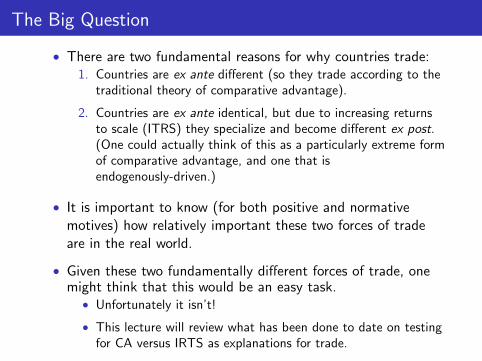
The Big Question

• There are two fundamental reasons for why countries trade: 1. Countries are ex ante different (so they trade according to the

traditional theory of comparative advantage).

2. Countries are ex ante identical, but due to increasing returns to scale (ITRS) they specialize and become different ex post. (One could actually think of this as a particularly extreme form of comparative advantage, and one that is endogenously-driven.)

• It is important to know (for both positive and normative motives) how relatively important these two forces of trade are in the real world.

• Given these two fundamentally different forces of trade, one might think that this would be an easy task.

• Unfortunately it isn’t!

• This lecture will review what has been done to date on testing for CA versus IRTS as explanations for trade.

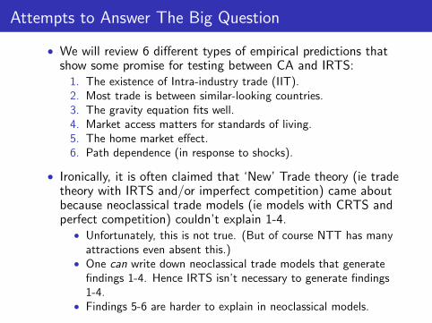
Attempts to Answer The Big Question

• We will review 6 different types of empirical predictions that show some promise for testing between CA and IRTS: 1. The existence of Intra-industry trade (IIT). 2. Most trade is between similar-looking countries. 3. The gravity equation fits well. 4. Market access matters for standards of living. 5. The home market effect. 6. Path dependence (in response to shocks).

• Ironically, it is often claimed that ‘New’ Trade theory (ie trade theory with IRTS and/or imperfect competition) came about because neoclassical trade models (ie models with CRTS and perfect competition) couldn’t explain 1-4.

• Unfortunately, this is not true. (But of course NTT has many attractions even absent this.)

• One can write down neoclassical trade models that generate findings 1-4. Hence IRTS isn’t necessary to generate findings 1-4.

• Findings 5-6 are harder to explain in neoclassical models.


1. Introduction







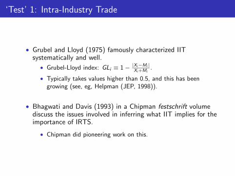
‘Test’ 1: Intra-Industry Trade

• Grubel and Lloyd (1975) famously characterized IIT systematically and well.

≡ 1 − |Xi −Mi |• Grubel-Lloyd index: GLi .Xi +Mi

• Typically takes values higher than 0.5, and this has been growing (see, eg, Helpman (JEP, 1998)).

• Bhagwati and Davis (1993) in a Chipman festschrift volume discuss the issues involved in inferring what IIT implies for the importance of IRTS.

• Chipman did pioneering work on this.

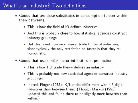
What is an industry? Two definitions

• Goods that are close substitutes in consumption (closer within than between).

• This is how the field of IO defines industries.

• And this is probably close to how statistical agencies construct industry groupings.

• But this is not how neoclassical trade thinks of industries, since typically the only restriction on tastes is that they’re homothetic.

• Goods that use similar factor intensities in production.

• This is how HO trade theory defines an industry.

• This is probably not how statistical agencies construct industry groupings.

• Indeed, Finger (1975): K/L ratios differ more within 3-digit industries than between them. (Though Maskus (1991) updated this and found there to be slightly more between than within.)

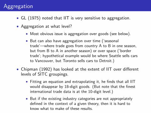
Aggregation

• GL (1975) noted that IIT is very sensitive to aggregation.

• Aggregation at what level?

• Most obvious issue is aggregation over goods (see below).

• But can also have aggregation over time (‘seasonal trade’—where trade goes from country A to B in one season, but from B to A in another season) or over space (‘border trade’; hypothetical example would be where Seattle sells cars to Vancouver, but Toronto sells cars to Detroit.)

• Chipman (1992) has looked at the extent of IIT over different levels of SITC groupings.

• Fitting an equation and extrapolating it, he finds that all IIT would disappear by 18-digit goods. (But note that the finest international trade data is at the 10-digit level.)

• But if the existing industry categories are not appropriately defined in the context of a given theory, then it is hard to know what to make of these results.

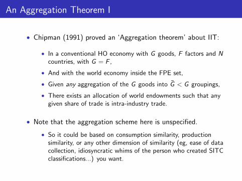
An Aggregation Theorem I

• Chipman (1991) proved an ‘Aggregation theorem’ about IIT:

• In a conventional HO economy with G goods, F factors and N countries, with G = F ,

• And with the world economy inside the FPE set,

• ¯Given any aggregation of the G goods into G < G groupings,

• There exists an allocation of world endowments such that any given share of trade is intra-industry trade.

• Note that the aggregation scheme here is unspecified.

• So it could be based on consumption similarity, production similarity, or any other dimension of similarity (eg, ease of data collection, idiosyncratic whims of the person who created SITC classifications...) you want.

An Aggregation Theorem II

• The intuition behind this result: • Imagine a perfectly symmetric world in which there is no trade. • Now let the countries exchange some of their relative

endowments such that incomes (and hence consumption patterns) remain unchanged. Production, however, will change.

• If the endowment change promotes production of good X in one country and good Y in the other country, and if goods X and Y are 2 goods that we’ve chosen to be inside the same ‘industry’ grouping, then the only trade that emerges is ‘intra-industry’.

• Note that ‘inside the FPE set’ is not innocuous here. • It requires that the A(w) matrix is non-singular, which requires

that each good G is using (even slightly) different factor intensities at w .

• So the two goods aggregated together into an industry can have ‘similar’, but not identical, factor intensities.

Chipman (1992)

• Chipman (1991) said that it is possible to get IIT in an HO model. But how much IIT should we expect in a ‘typical’ HO model?

• Chipman (1992) works with a simple example, but the intuition that emerges is, ‘a lot’.

• That is, IIT is likely to be the rule rather than the exception in an HO-style model.

• The basic intuition is that as the technologies for making 2 goods become more similar, the PPF becomes flatter, which gives rise to more specialization.

• So if we group goods into ‘industries’ based on production similarity, there will be lots of scope for intra-industry specialization within these groupings, and hence lots of scope for IIT.

• Rodgers (1988) extended this in a more formal direction, defining production similarity on a Euclidian norm operating on Cobb-Douglas elasticities.

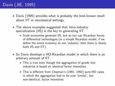
Davis (JIE, 1995)

• Davis (1995) provides what is probably the best-known result about IIT in neoclassical settings.

• The above examples suggested that intra-industry specialization (IIS) is the key to generating IIT.

• Scale economies generate IIS, but so too can Ricardian forces of differential technologies (in a simple Ricardian model, if we define the entire economy as one ‘industry’ then there is clearly both IIS and IIT).

• So Davis develops a HO-Ricardian model in which there is an arbitrary amount of IIT.

• This is true even though the aggregation of goods into industries is based on identical factor intensities.

• This is different from Chipman’s (1991, 1992) pure-HO cases in which the aggregation had to be over ‘similar’, but non-identical, factor intensities.

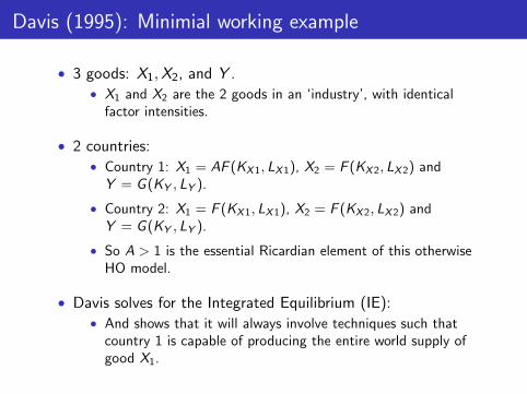
Davis (1995): Minimial working example

• 3 goods: X1, X2, and Y . • X1 and X2 are the 2 goods in an ‘industry’, with identical

factor intensities.

• 2 countries: • Country 1: X1 = AF (KX 1, LX 1), X2 = F (KX 2, LX 2) and

Y = G (KY , LY ).

• Country 2: X1 = F (KX 1, LX 1), X2 = F (KX 2, LX 2) and Y = G (KY , LY ).

• So A > 1 is the essential Ricardian element of this otherwise HO model.

• Davis solves for the Integrated Equilibrium (IE): • And shows that it will always involve techniques such that

country 1 is capable of producing the entire world supply of good X1.

210 D.R. Davis I Journal of International Economics 39 (1995) 201-226

kxl = kx2

Fig. 1. The integrated equilibrium.

Eing the integrated equilibrium technique. This is reflected by the vector V(1) that extends from 0, with slope k,, , reflecting total factor usage in good X,. Taking this factor requirement as a new vertex for country One, the equilibrium techniques used in production of goods X2 and Y give rise to cones for the two countries in factor space. Any division of the world factor endowment that falls within the parallelogram generated by the intersection of these two cones allows replication of the integrated equilibrium.

The FPE set Point V (1) is the vector of factors the IE would use to make good 1, which is then the new origin for country 1.

Figure from Davis, Donald. "Intra-industry Trade: A Heckscher-Ohlin-Ricardo Approach." Journal of International Economics 39, no. 3 (1995): 201-26. Courtesy of Elsevier. Used with permission.

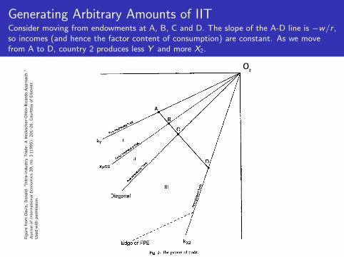
Generating Arbitrary Amounts of IIT Consider moving from endowments at A, B, C and D. The slope of the A-D line is −w/r , so incomes (and hence the factor content of consumption) are constant. As we move from A to D, country 2 produces less Y and more X2.

o

Figure

fro

m D

avis

, D

onal

d.

"Intr

a-in

dust

ry T

rade:

A H

ecks

cher

-Ohlin

-Ric

ardo A

ppro

ach."

Jour

nal o

f In

tern

atio

nal E

cono

mic

s 39,

no.

3 (

1995):

201-2

6.

Court

esy

of

Els

evie

r.U

sed w

ith p

erm

issi

on.

2

Davis (1995): A final point

• It has often been argued that product differentiation and IIT go hand in hand.

• Eg: Grubel-Lloyd (1975) subtitle: The theory and measurement of international trade in differentiated products.

• And product differentiation and IRTS are often argued to go hand in hand.

• But Davis (1995) points out that a rise in the number of products G relative to factors F (ie the presence of G > F , which we might think of as ‘product differentiation’) also makes any technology differences across countries more likely to generate IIT (even with CRTS).


1. Introduction







‘Test’ 2: Most trade is North-North; or, most trade is between similar-looking countries.

• It was never formally claimed that this could never happen in a neoclassical model.

• Key obstacle is that, with more than 2 countries, neoclassical models typically don’t make bilateral predictions about who trades with whom.

• Though non-FPE versions of the H-O model, like that in Helpman (1984), are exception, and do make bilateral statements.

• Davis (JPE, 1997):

• Showed in an elegant and transparent manner how endowment differences translate into trade flow differences.

• He hence documented the conditions under which, even in a pure HO model, similarly-endowed countries trade less with one another than do differently-endowed countries.

Davis (JPE, 1997)

• Consider a 4 × 4 × 4 framework:

• 2 Northern countries, 2 Southern countries.

• Northern countries relatively endowed with ‘North-type’ factors. Endowments inside FPE set.

• 2 ‘North-type’ industries (to be defined shortly), and 2 ‘South-type’ industries.

__

__

Davis (JPE, 1997)

⎤ ⎥⎥⎦

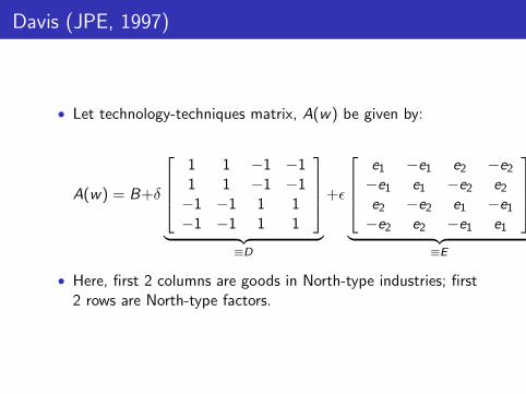
• Let technology-techniques matrix, A(w) be given by:

⎡⎤⎡ 1 1 −1 −1 e1 −e1 e2 −e2 ⎢⎢⎣

⎥⎥⎦+E⎢⎢⎣

−e1 e1 −e2 e2

e2 −e2 e1 −e1

1 1 −1 −1A(w) = B+δ −1 −1 1 1

−1 −1 1 1 −e2 e2 −e1 e1 ≡D ≡E

• Here, first 2 columns are goods in North-type industries; first 2 rows are North-type factors.

=

A B + δD + �E

• So the B matrix represents ‘average’ input coefficients.

• The D matrix represents technological dispersion between industries.

• The E matrix represents technological dispersion within industries

• And then the notion of an ‘industry’ (based on technological similarity) comes from conditions which (are not unambiguous but) generally require δ to exceed a mixture of E and e1 and e2.

• That is, there is more dispersion in A between industries than within.

Davis (1997): Results

• From this, Davis (1997) shows that the HOV equations imply the following: 1. V N − V S = 2tNS δD1 (where tNS is the total trade volume of

the North with the South, and D1 is the first row of D). 2. V N − V N = 2tNN EE1 (defined similarly).

• Hence, for fixed endowment differences, the volumes of trade depend critically on δ and E. 1. If the goods in which N and S specialize are very different in

their input intensities (high δ) then only a small amount of trade (low tNS ) is needed to accomplish the required amount of factor trade.

2. If the goods in which N and N’ specialize are very similar (low ε) then even though the net content of factor services traded will be small, there is lots of back-and-forth factor services trade, which is accomplished by lots of goods trade (high tNN ).

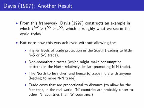
Davis (1997): Another Result

• From this framework, Davis (1997) constructs an example in > tNSwhich tNN > tSS , which is roughly what we see in the

world today.

• But note how this was achieved without allowing for:

• Higher levels of trade protection in the South (leading to little N-S or S-S trade).

• Non-homothetic tastes (which might make consumption patterns in the North relatively similar, promoting N-N trade).

• The North to be richer, and hence to trade more with anyone (leading to more N-N trade).

• Trade costs that are proportional to distance (to allow for the fact that, in the real world, ‘N’ countries are probably closer to other ‘N’ countries than ‘S’ countries.)

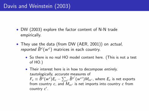
Davis and Weinstein (2003)

• DW (2003) explore the factor content of N-N trade empirically.

• They use the data (from DW (AER, 2001)) on actual, reported B̄ c (w c ) matrices in each country.

• So there is no real HO model content here. (This is not a test of HO.)

• Their interest here is in how to decompose entirely, tautologically, accurate measures of r Fc ≡ B̄ c (w c )Ec − B̄ c1

(w c ')Mcc1 , where Ec is net exports 1c1from country c , and Mcc is net imports into country c from

'country c .

DW (2003) Results

1. The pure intra-industry component of Fc is significant (42 % of all Fc ).

• In a conventional HO model (with FPE) there is no IIT FCT.

• In fact, as discussed above, the existence of IIT has been taken as evidence against the HO model.

• But in this setting, where the B̄ c (w c ) matrices are allowed to differ (and, strikingly, do differ) we see that, even within the richest countries in the OECD, IIT is a conduit for much factor services trade.

2. For the median G10 country, lots of factor services trade is within the North.

• For K: 48 % is within North. • For L: 37 % is within North.


1. Introduction







The Gravity Equation

• The gravity equation is one of the best fitting and most established empirical relationships in all of Trade.

• Though as an aside (which we will see more of in a later lecture), Trefler and Lai (2002) demonstrate how the segments of the variation that the gravity equation fits well require only assumptions that virtually any economic model would maintain (eg market clearing).

• For a long time, the impressive fit of the gravity equation was seen as evidence for the importance of IRTS in trade.

• This is partly because Helpman (1987) and Bergstrand (ReStat, 1989) showed how elegantly the monopolistic competition theory of trade (eg Helpman and Krugman (1985)) could be manipulated into a gravity equation form.

• But really, the field had known since at least Anderson (AER, 1979) that the Armington model could deliver a gravity equation, and the Armington model is really just an extreme Ricardian model. (We’ll see more of the Armington model in a later lecture.)

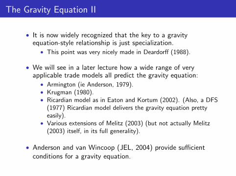
The Gravity Equation II

• It is now widely recognized that the key to a gravity equation-style relationship is just specialization.

• This point was very nicely made in Deardorff (1988).

• We will see in a later lecture how a wide range of very applicable trade models all predict the gravity equation:

• Armington (ie Anderson, 1979). • Krugman (1980). • Ricardian model as in Eaton and Kortum (2002). (Also, a DFS

(1977) Ricardian model delivers the gravity equation pretty easily).

• Various extensions of Melitz (2003) (but not actually Melitz (2003) itself, in its full generality).

• Anderson and van Wincoop (JEL, 2004) provide sufficient conditions for a gravity equation.

The Gravity Equation III

• Deardorff (1998) also discusses how the HO model has gravity-like features to it.

• At first glance this is surprising, since bilateral trade isn’t pinned down in the HO model.

• But Deardorff points out that bilateral trade isn’t determined because buyers are indifferent about where they buy from.

• So if buyers (somewhat plausibly?) settled this indifference randomly, and in proportion to the ‘number’ of sellers offering them goods from each country, the resulting bilateral trades would be gravity-like.

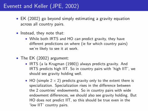
Evenett and Keller (JPE, 2002)

• EK (2002) go beyond simply estimating a gravity equation across all country pairs.

• Instead, they note that: • While both IRTS and HO can predict gravity, they have

different predictions on where (ie for which country pairs) we’re likely to see it at work.

• The EK (2002) argument: • IRTS (a la Krugman (1980)) always predicts gravity. And

IRTS predicts high IIT. So in country pairs with ‘high IIT’, we should see gravity holding well.

• HO (simple 2 × 2) predicts gravity only to the extent there is specialization. Specialization rises in the difference between the 2 countries’ endowments. So in country pairs with wide endowment differences, we should also see gravity holding. But HO does not predict IIT, so this should be true even in the ‘low IIT’ country pairs.

EK (2002): 4 Models

• They compare 4 models: Yi Yj1. Pure-IRTS: Complete specialization, so Mij = α YW with

α = 1. This is true in high-IIT samples, and more true as IIT rises.

2. Pure-HO with complete specialization (‘multicone HO’): so again α = 1. But this is in low-IIT samples, and more true as endowment differences (‘FDIF’) rise.

3. Mix HO-IRTS (a la Helpman and Krugman (1985)): now α = 1 − γ i , and γ i being the share of GDP that is in the CRTS sector. This is true in high-IIT samples, and more true as IIT rises.

4. Pure HO with incomplete specialization (‘unicone HO’): now α = γ i − γj , with γ i being the share of GDP in one of the 2 sectors. This is in low-IIT samples, and more true as endowment differences (‘FDIF’) rise.

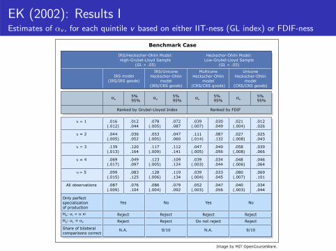
EK (2002): Results I Estimates of αv , for each quintile v based on either IIT-ness (GL index) or FDIF-ness

Benchmark Case

IRS/Unicone Heckscher-Ohlin

model (IRS/CRS goods)

Heckscher-Ohlin Model: Low-Grubel-Lloyd Sample

(GL < .05)

IRS/Heckscher-Ohlin Model: High-Grubel-Lloyd Sample

(GL > .05)

Unicone Heckscher-Ohlin

model (CRS/CRS goods)

Multicone Heckscher-Ohlin

model (CRS/CRS goods)

IRS model (IRS/IRS goods)

αυ 5% 95%

αυ 5% 95%

αυ 5% 95%

αυ 5% 95%

Ranked by Grubel-Lloyed Index Ranked by FDIF

υ = 1 .016 (.012) .044

.012 (.005) .078

.087

.072 (.007) .039

.049

.030 (.004) .021

.026

.012

υ = 2 .044 (.005) .052

.036 (.005) .053

.060

.047 (.014) .111

.132

.087 (.008) .027

.043

.025

υ = 3 (.013) .139

.164

.120 (.009) .117

.141

.112 (.005) .047

.056

.040 (.008) .058

.066

.039

υ = 4 (.017) .069

.097

.049 (.005) .123

.124

.109 (.003) .039

.044

.034 (.006) .048 .046

.064

υ = 5 (.015) .099

.125

.083 (.006) .128

.134

.119 (.004) .039

.045

.033 (.007) .080

.101

.069

All observations (.009) .087

.104

.076 (.004) .086

.092

.079 (.003) .052

.056

.047 (.003) .040 .034

.044

Only perfect specialization of production

Yes No Yes No

H0: αi = α A

i Reject Reject Reject Reject

H0: α1 = α5 Reject Reject Do not reject Reject

Share of bilateral comparisons correct

N.A. 9/10 N.A. 9/10

Image by MIT OpenCourseWare.

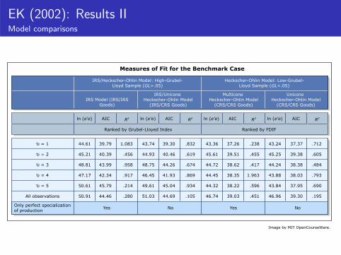
EK (2002): Results II Model comparisons

Measures of Fit for the Benchmark Case

IRS Model (IRS/IRS Goods)

IRS/Unicone Heckscher-Ohlin Model

(IRS/CRS Goods)

Unicone Heckscher-Ohlin Model

(CRS/CRS Goods)

Multicone Heckscher-Ohlin Model

(CRS/CRS Goods)

IRS/Heckscher-Ohlin Model: High-Grubel-Lloyd Sample (GL>.05)

Heckscher-Ohlin Model: Low-Grubel-Lloyd Sample (GL<.05)

ln (e'e) AIC R2 ln (e'e) AIC R2 ln (e'e) AIC R2 ln (e'e) AIC R2

Ranked by Grubel-Lloyed Index Ranked by FDIF

υ = 1 44.61 39.79 1.083 43.74 39.30 .832 43.36 37.26 .238 43.24 37.37 .712

υ = 2 45.21 40.39 .456 44.93 40.46 .619 45.61 39.51 .455 45.25 39.38 .605

υ = 3 48.81 43.99 .958 48.75 44.26 .674 44.72 38.62 .417 44.24 38.38 .484

υ = 4 47.17 42.34 .917 46.45 41.93 .869 44.45 38.35 1.963 43.88 38.03 .793

υ = 5 50.61 45.79 .214 49.61 45.04 .934 44.32 38.22 .596 43.84 37.95 .690

All observations 50.91 44.46 .280 51.03 44.69 .105 46.74 39.03 .451 46.96 39.30 .195

Only perfect specialization of production

Yes No Yes No



1. Introduction







‘Test’ 4: Market Size matters

• Two tests of this:

• Redding and Venables (JIE, 2004): does measured ‘market access’ (as measured from the fixed effects in a gravity equation) predict Y/L? Yes.

• Redding and Sturm (AER, 2008): When Germany was partitioned, did cities on the Eastern edge of West Germany (who lost market access) suffer? Did they recover when Germany was re-unified? Does ‘market access’ predict the magnitude of these effects? Yes, yes and yes.

• Unfortunately, the models used to generate a ‘market access’ term in these papers are all effectively ‘gravity models’, which (as discussed above) is a class of models that includes both IRTS and neoclassical variants. So the demonstrated evidence that ‘market size matters’ can’t be taken as evidence for IRTS over neoclassical forces.

5.3. Economic geography and per capita income: preferred specification

We now move on to present our preferred specification of the relationship between

economic geography and per capita income, where we control for cross-country variation

Fig. 2. GDP per capita and MA=DMA(1) + FMA.

Fig. 3. GDP per capita and MA=DMA(2) + FMA.

S. Redding, A.J. Venables / Journal of International Economics 62 (2004) 53–82 67

Redding and Venables (2004): Results MA (‘Market access’) is constructed using an inverse trade-cost weighted sum of gravity equation fixed effects.

Figure from Redding, Stephen, and Anthony Venables. "Economic Geography and International Inequality." Journal of Political Economy 62, no. 1 (2004): 53-82. Courtesy of Elsevier. Used with permission.

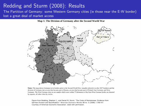
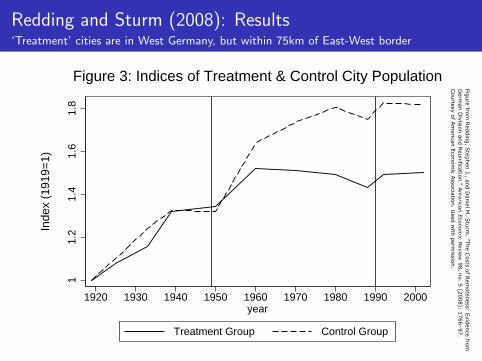
Map 1: The Division of Germany after the Second World War

Notes: The map shows Germany in its borders prior to the Second World War (usually referred to as the 1937 borders) and the division of Germany into an area that became part of Russia, an area that became part of Poland, East Germany and West Germany. The West German cities in our sample which were within 75 kilometers of the East-West German border are denoted by squares, all other cities by circles.

Redding and Sturm (2008): Results The Partition of Germany: some Western Germany cities (ie those near the E-W border) lost a great deal of market access

Figure from Redding, Stephen J., and Daniel M. Sturm. "The Costs of Remoteness: Evidence from German Division and Reunification." American Economic Review 98 no. 5 (2008): 1766–97. Courtesy of American Economic Association. Used with permission.

Figures 3 and 4

11.

21.

41.

61.

8

1920 1930 1940 1950 1960 1970 1980 1990 2000year

Treatment Group Control Group

Inde

x (1

919=

1)

Figure 3: Indices of Treatment & Control City Population−

0.3

−0.

2−

0.1

0.0

1920 1930 1940 1950 1960 1970 1980 1990 2000year

Tre

atm

ent G

roup

− C

ontr

ol G

roup

Figure 4: Difference in Population Indices, Treatment − Control

Figure fro

m R

eddin

g, S

tephen

J., and D

aniel M

. Stu

rm. "T

he C

osts o

f Rem

oten

ess: Evid

ence fro

mG

erman

Divisio

n an

d R

eunificatio

n." A

merican Econom

ic Review

98, n

o. 5

(2008): 1

766–97.

Courtesy o

f Am

erican E

conom

ic Asso

ciation. U

sed w

ith p

ermissio

n.

Redding and Sturm (2008): Results ‘Treatment’ cities are in West Germany, but within 75km of East-West border


1. Introduction







Test 5: The Home Market Effect

• Recall the HME (as in Krugman, 1980):

• In a 2-country world, with at least one sector featuring IRTS and transport costs, and FPE holding (driven in Krugman (1980) by the assumption of a perfectly competitive, homogeneous, zero-trade cost outside good), the country with higher relative demand for the IRTS good will export that good.


• The HME has been characterized as one particularly novel finding to emerge from IRTS theories of trade.

• In particular, in a CRTS world (with trade costs or not), it would be strange for an increase in a country’s relative demand for a good to cause that country to export more of the good.

• This is actually possible in a CRTS world, but would require very perverse import demand and export supply curves.

• HME is important, not just for distinguishing IRTS from CRTS in Trade theory:

• Important policy ramifications if HME is true.

• All of the ‘New’ Economic Geography (really, models of agglomeration based on pecuniary externalities through trade costs, as opposed to non-pecuniary externalities like knowledge spillovers) literature relies on the HME.


• So testing for the HME is attractive as a test for the importance of IRTS in trade.

• Unfortunately, testing for it is not trivial.

• We would like to nest it in an otherwise standard neoclassical model, which is hard.

• We would like to generalize it to many countries/industries, which is hard.

• We would like to drop the FPE assumption but this is also hard.

• Despite these difficulties, researchers have made progress here:

• Davis and Weinstein (JIE, 2003)

• Hanson and Xiang (AER, 2004)

• Behrens et al (2009)

Davis and Weinstein (2003)

• NB: A lot of what is going on in this paper is explained more fully in DW (1996, working paper).

• DW (2003) use data on OECD manufacturing and try to nest H-O with a version of Krugman (1980) that delivers an HME.

• They focus on the implications of the HME for production rather than exporting behavior, but the same intuition goes through for exporting.

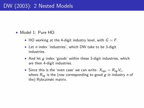
DW (2003): 2 Nested Models

• Model 1: Pure HO:

• HO working at the 4-digit industry level, with G = F .

• Let n index ‘industries’, which DW take to be 3-digit industries.

• And let g index ‘goods’ within these 3-digit industries, which are then 4-digit industries.

• Since this is the ‘even case’ we can write: Xngc = Rng Vc , where Rng is the (row corresponding to good g in industry n of the) Rybczinski matrix.

� � � �

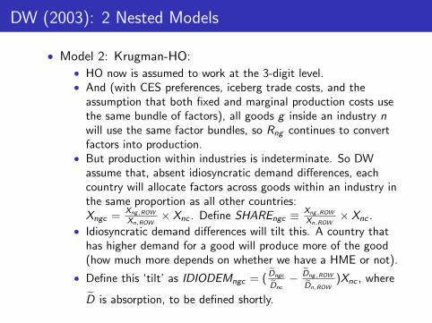
DW (2003): 2 Nested Models

• Model 2: Krugman-HO: • HO now is assumed to work at the 3-digit level. • And (with CES preferences, iceberg trade costs, and the

assumption that both fixed and marginal production costs use the same bundle of factors), all goods g inside an industry n will use the same factor bundles, so Rng continues to convert factors into production.

• But production within industries is indeterminate. So DW assume that, absent idiosyncratic demand differences, each country will allocate factors across goods within an industry in the same proportion as all other countries:

Xng ,ROW Xng ,ROW Xngc = × Xnc . Define SHAREngc ≡ × Xnc .Xn,ROW Xn,ROW

• Idiosyncratic demand differences will tilt this. A country that has higher demand for a good will produce more of the good (how much more depends on whether we have a HME or not).

D Dngc ng,ROW • Define this ‘tilt’ as IDIODEMngc = ( − )Xnc , where Dnc Dn,ROW

D� is absorption, to be defined shortly.

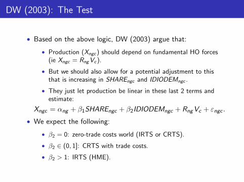
DW (2003): The Test

• Based on the above logic, DW (2003) argue that:

• Production (Xngc ) should depend on fundamental HO forces (ie Xngc = Rng Vc ).

• But we should also allow for a potential adjustment to this that is increasing in SHAREngc and IDIODEMngc .

• They just let production be linear in these last 2 terms and estimate:

Xngc = αng + β1SHAREngc + β2IDIODEMngc + Rng Vc + εngc .

• We expect the following:

• β2 = 0: zero-trade costs world (IRTS or CRTS).

• β2 ∈ (0, 1]: CRTS with trade costs.

• β2 > 1: IRTS (HME).

DW (2003): Constructing SHAREngc

• How do we measure a country’s total ‘demand’ (really, absorption) for a good, ie D�

ngc ? • DW (1996) used simply the amount of local demand in

country c for this good g in industry n. • DW (2003) instead use the derived demand for country c ’s

goods both at home and in its trading partners as well. To measure this they first regress, industry-by-industry, a gravity equation to get the effect of distance on demand. From this they can sum over all trade partners, down-weighting by distance, to get a sense of the ‘market size’ for g , n faced by country c .

• This distinction turns out to have big effects.

• An important concern is simultaneity bias: do un-modeled production differences drive idiosyncratic demand differences (for example, by changing prices, or even tastes?)

• DW use lagged (by 15 years) demand data to try to mitigate this.

• Various other discussions in text.

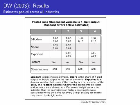
DW (2003): Results Estimates pooled across all industries

Pooled runs (Dependent variable is 4-digit output; standard errors below estimates)

1 2 3 4

Idiodem 1.67 0.05

1.67 0.05

1.57 0.10

1.57 0.10

Share 0.96 0.01

0.92 0.02

Exported 0.02 0.07 0.01

0.04

Factors No No Yes Yes

Observations 650 650 650 650

Idiodem is idiosyncratic demand, Share is the share of 4-digit output in 3-digit output in the rest of the world, Exported is a dummy variable that is one if the country is a net exporter of the good, and Factors indicates whether the coefficients on factor endowments were allowed to differ across 4-digit sectors. No indicates that the coefficients on factor endowments were constrained to be the same for every 3-digit sector; Yes means they varied by 4-digit sector.


DW (2003): Interpretation

• Strong evidence for β2 > 1, so an HME.

• Endowments account for around 50 % of production variation, and CRTS around 30 %.

• Running this regression industry-by-industry reveals that β2 > 1 in around half of the industries. At face value, these are not obviously the industries where you might expect to see the strongest tendency for an HME.

• This contrasts starkly with DW (1996), which used only local demand to construct D, where β2 = 0.3.

• In parallel work, DW (EER, 1999) did a similar exercise to DW (1996) on Japanese regions and estimated β2 = 0.9, which suggests greater scope for an HME within countries.

• Though these results are hard to compare with DW (1996, 2003) since the Japanese data are at a coarser level of industry aggregation.

Hanson and Xiang (AER, 2004)

• Hanson and Xiang (2004) is probably the most cited paper with reference to evidence for the HME.

• HX construct a Krugman (1980)-style model that makes predictions about which industries are more likely exhibit an HME, and then looks for that in export data.

• A nice feature is its ‘difference-in-difference’ design, which is there to try to difference out some unobserved and/or endogenous terms.

HX (2004): 2-country model

• They build intuition for their main, multi-country empirical specification by developing a 2-country model with many industries.

• 2 countries (H and F), with LH > LF .

• A continuum of industries (z), each of which is a Krugman (1980) sector (ie a continuum of varieties, with Dixit-Stiglitz tastes, CES parameter σ(z) and trade costs τ(z).)

• Have to restrict technologies a bit to simplify the cross-industry specialization. Recall the goal here is to get an industry-level prediction on how much HME there is in industry z .

HX (2004): 2-country model

• Can then derive the following intuitive results (where T and C are meant to make you think of ‘treatment’ and ‘control’):

1. Say that there is a larger HME in industry T than in C iff nH (T )/nF (T ) > nH (C )/nF (C ) > LH /LF , where n is the number of varieties (recall that with CES the output per variety is the same everywhere, so counting varieties is what matters).

2. Then, if industries T and C are such that τ(C )1−σ(C ) = τ(T )1−σ(T ), but σ(C ) > σ(T ) then there will be a larger HME in industry T than in C .

3. Likewise, if industries T and C are such that τ(C )1−σ(C ) = τ(T )1−σ(T ), but τ (C ) < τ (T ) then there will be a larger HME in industry T than in C .

HX (2004): N-country model

• HX (2004) then consider an N-country model, with a discrete number of industries.

• The only other modification is to write trade costs (from i icountry j to country k in industry k) as: τjk = tjk (djk )

γi , iwhere tjk is the tariff on this trade and djk is the distance

between j and k.

• They then show the following (which is a simple matter of writing down CES demand functions and substituting in the very simple supply side of a Krugman (1980) model):

ST /ST T T T T )1−σT jk hk nj /nh (wj /wh

= (djk /dhk )(1−σT )γT −(1−σC )γC

CSC /SC nC /n (wC /wC )1−σC jk hk j h j h

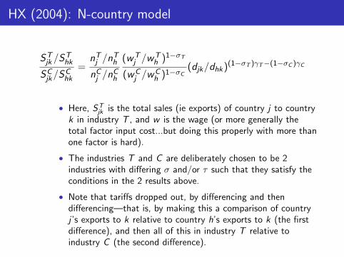
HX (2004): N-country model

ST /ST T T T T )1−σT jk hk nj /nh (wj /wh

= (djk /dhk )(1−σT )γT −(1−σC )γC

CSC /SC nC /n (wC /wC )1−σC jk hk j h j h

• Here, SjkT is the total sales (ie exports) of country j to country

k in industry T , and w is the wage (or more generally the total factor input cost...but doing this properly with more than one factor is hard).

• The industries T and C are deliberately chosen to be 2 industries with differing σ and/or τ such that they satisfy the conditions in the 2 results above.

• Note that tariffs dropped out, by differencing and then differencing—that is, by making this a comparison of country j ’s exports to k relative to country h’s exports to k (the first difference), and then all of this in industry T relative to industry C (the second difference).

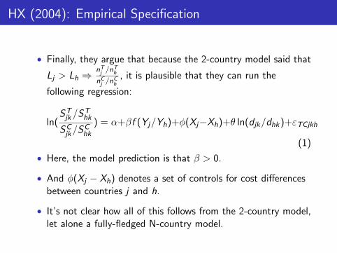
HX (2004): Empirical Specification

• Finally, they argue that because the 2-country model said that Tnj

T /nhLj > Lh ⇒ n /n

, it is plausible that they can run the C C j h

following regression:

ST /ST jk hk

ln( ) = α+βf (Yj /Yh)+φ(Xj −Xh)+θ ln(djk /dhk )+εTCjkhSC /SC jk hk

(1)

• Here, the model prediction is that β > 0.

• And φ(Xj − Xh) denotes a set of controls for cost differences between countries j and h.

• It’s not clear how all of this follows from the 2-country model, let alone a fully-fledged N-country model.

H

anso

n,

Gord

on H

., a

nd C

hong X

iang.

"The

Hom

e-M

arke

t Eff

ect

and B

ilate

ral Tra

de

Patt

erns.

" Am

eric

an E

cono

mic

Rev

iew

94,

no.

4 (

2004):

1108–29.

Court

esy

of

Am

eric

an E

conom

ic A

ssoci

atio

n.

Use

d w

ith p

erm

issi

on.

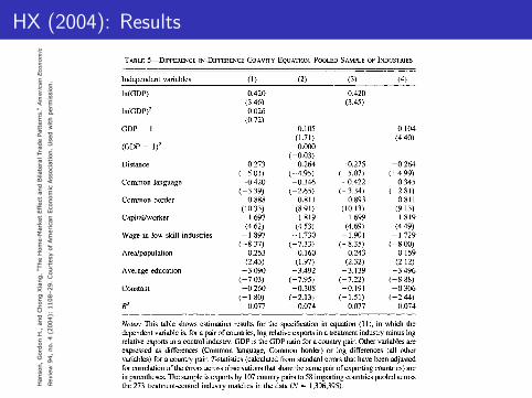
HX (2004): Results THE AMERICAN ECONOMIC REVIEW

TABLE 5-DIFFERENCE-IN-DIFFERENCE GRAVITY EQUATION, POOLED SAMPLE OF INDUSTRIES

Independent variables (1) (2) (3) (4)

ln(GDP) 0.420 0.420 (3.46) (3.45)

ln(GDP)2 0.026 (0.72)

GDP- 1 0.105 0.104 (1.71) (4.40)

(GDP - 1)2 0.000

(-0.03) Distance -0.273 -0.264 -0.275 -0.264

(-5.01) (-4.95) (-5.07) (-4.99) Common language -0.420 -0.346 -0.422 -0.345

(-3.39) (-2.65) (-3.34) (-2.81) Common border 0.888 0.811 0.893 0.811

(10.33) (8.91) (10.13) (9.13) Capital/worker 1.697 1.819 1.699 1.819

(4.62) (4.53) (4.69) (4.49) Wage in low-skill industries -1.897 -1.730 -1.901 -1.729

(-8.37) (-7.33) (-8.35) (-8.00) Area/population 0.253 0.160 0.243 0.159

(2.43) (1.97) (2.32) (2.12) Average education -3.090 -3.492 -3.139 -3.496

(-7.03) (-7.95) (-7.22) (-8.88) Constant -0.260 -0.308 -0.191 -0.306

(-1.80) (-2.13) (-1.51) (-2.44) R2 0.077 0.074 0.077 0.074

Notes: This table shows estimation results for the specification in equation (11), in which the dependent variable is, for a pair of countries, log relative exports in a treatment industry minus log relative exports in a control industry. GDP is the GDP ratio for a country pair. Other variables are expressed as differences (Common language, Common border) or log differences (all other variables) for a country pair. T-statistics (calculated from standard errors that have been adjusted for correlation of the errors across observations that share the same pair of exporting countries) are in parentheses. The sample is exports by 107 country pairs to 58 importing countries pooled across the 273 treatment-control industry matches in the data (N = 1,396,395).

term (nmj/lmh)l(nioj/loh)

in equation (10), with an

increasing function that is linear in polynomials of (YjYh - 1) or ln(YjIYh). This approximation result gives us the specification in equation (11), in which relative exports are a function of relative exporter size. In Table 5, we experiment with functional forms forf() in equation (11). Column (1) includes ln(YjlYh) and its square as regressors, column (2) includes (YjYh - 1) and its square as regressors, and columns (3) and (4) include ln(YJYh) or (Y/Yh - 1) alone.

In all regressions, relative exports are increasing in relative exporter GDP. This implies that larger countries export more of high transport cost, low-o- goods relative to their exports of low transport cost, high-o goods and is consistent with a home-market effect as stated in Propositions 1 and 2. The square terms on relative exporter size are statistically insignificant (as are higher order polynomials) and we drop

them in later regressions. The coefficient estimate on ln(YJ/Yh) is precisely estimated in all specifications and the coefficient estimates on

(YjlYh - 1) is precisely estimated when its

square is excluded as a regressor. Since the specification with log relative exporter GDP is closest to the standard gravity model, we adopt column (3) as our preferred specification. In this specification, log relative exporter GDP has a coefficient estimate of 0.42. This implies that if one exporter is 10 percent larger than another exporter, then the larger country will on average have export shipments of high transport cost, low-a goods that are 4.2 percent higher than the shipments of the smaller country, where these values are normalized by the two countries' relative shipments of low transport cost, high-o- goods.

Coefficient estimates on other regressors are consistent with results from gravity model esti-

SEPTEMBER 2004 1120

Other work on the HME

• Head and Ries (AER, 2001): • Studying which firms expanded and contracted in Canada

around NAFTA.

• Behrens , Lamorgese, Ottaviano and Tabuchi (2009):

• Point out that extending Krugman (1980) from 2 to N countries is hard, and that the simple HME doesn’t survive.

• This also casts doubt on Hanson and Xiang (2004) extension from 2 to N countries.


1. Introduction







Test 6: Path Dependence

• Under certain conditions, models of IRTS can generate path dependence: initial, random advantage can become permanent.

• This is what happens when the HME (in Krugman 1980) is combined with factor mobility (as Krugman (JPE, 1991) did to great effect).

• Tests of path dependence (have been contradictory!):

• Davis and Weinstein (AER, 2002): Did city population shares in Japan return to normal after WWII bombing? Yes.

• Davis and Weinstein (JRS, 2008): Did city-by-industry manufacturing output/employment shares do the same? Yes.

• Bleakley and Lin (2010): Is current US population clustered in places that have natural resources that were previously productive, but are no longer of any productive use? Yes.

Davis and Weinstein (2002) The big two returned to normal

THE AMERICAN ECONOMIC REVIEW

c 0o

a. 0

o

1925 1930 1935 1940 1947 1950 1955 1960 1965 1970 1975

Year

FIGURE 2. POPULATION GROWTH

wartime growth should asymptotically approach unity as the end period increases. In the last column of Table 3 we repeat the regression, only now extending the endpoint to 1965 instead of 1960. The estimated coefficient now reaches -1.027. That is, after controlling for prewar growth trends, by 1965 cities have entirely reversed the damage due to the war. Again, the impact of reconstruction subsidies also lessens as we move into the future. To- gether, these results suggest that the effect of the temporary shocks vanishes completely in less than 20 years.

One possible objection to our interpretation is that in most cases, the population changes cor- responded much more to refugees than deaths. Of the 144 cities with positive casualties, the average number of deaths per capita was only 1 percent. Most of the population movement that we observe in our data is due to the fact that the vast destruction of buildings forced people to live elsewhere. However, forcing them to move out of their cities for a number of years may not have sufficed to overcome the social networks and other draws of their home cities. Hence it may seem uncertain whether they are moving back to take advantage of particular character- istics of these locations or simply moving back to the only real home they have known.

However, there are two cases in which this argument cannot be made: Hiroshima and Na-

gasaki. In those cities, the number of deaths was such that if these cities recovered their populations, it could not be because residents who temporarily moved out of the city returned in subsequent years. We have already noted that our data underestimates casualties in these cities. Even so, our data suggest that the nuclear bombs immediately killed 8.5 percent of Na- gasaki's population and 20.8 percent of Hiro- shima's population. Moreover given that many Japanese were worried about radiation poison- ing and actively discriminated against atomic bomb victims, it is unlikely that residents felt an unusually strong attachment to these cities or that other Japanese felt a strong desire to move there. Another reason why these cities are in- teresting to consider is that they were not particularly large or famous cities in Japan. Their 1940 populations made them the 8th and 12th largest cities in Japan. Both cities were close to other cities of comparable size so that it would have been relatively easy for other cities to absorb the populations of these devastated cities.

In Figure 2 we plot the population of these two cities. What is striking in the graph is that even in these two cities there is a clear indica- tion that they returned to their prewar growth trends. This process seems to have taken a little longer in Hiroshima than in other cities, but this is not surprising given the level of destruction.

1282 DECEMBER 2002

Davis, Donald R., and David E. Weinstein. "Bones, Bombs, and Break Points: The Geography of Economic Activity." American Economic Review 92, no. 5 (2002): 1269–89. Courtesy of American Economic Association. Used with permission.

Dav

is,

Donal

d R

., a

nd D

avid

E.

Wei

nst

ein.

"Bones

, Bom

bs,

and B

reak

Poin

ts:

The

Geo

gra

phy

of

Eco

nom

ic A

ctiv

ity.

" Am

eric

an E

cono

mic

Rev

iew

92,

no.

5 (

2002):

1269–89.

Court

esy

of

Am

eric

an E

conom

ic A

ssoci

atio

n.

Use

d w

ith p

erm

issi

on.

Davis and Weinstein (2002) And in general, we see mean reversion (ie the opposite of path dependence) THE AMERICAN ECONOMIC REVIEW

(5) Sit+1 = Sit + 12it?I*

If p E [0, 1), then city share is stationary and any shock will dissipate over time. In other words, these two hypotheses can be distin- guished by identifying the parameter p.

One approach to investigating the magnitude of p is to search for a unit root. It is well known that unit root tests usually have little power to separate p < 1 from p = 1. This is due to the fact that in traditional unit root tests the innovations are not observable and so identify p with very large standard errors. A major advantage of our data set is that we can easily identify the innovations due to bombing. In particular, since by hypothesis the innovation, vit, is uncorre- lated with the error term (in square brackets), then if we can identify the innovation, we can obtain an unbiased estimate of p.

An obvious method of looking at the innovation is to use the growth rate from 1940 to 1947. However, this measure of the innovation may contain not only information about the bombing but also past growth rates. This is a measurement error problem that could bias our estimates in either direction depending on p. In order to solve this, we instrument the growth rate from 1940-1947 with buildings destroyed per capita and deaths per capita.20

We can obtain a feel for the data by considering the impact of bombing on city growth rates. As we argued earlier, if city growth rates follow a random walk, then all shocks to cities should be permanent. In this case, one should expect to see no relationship between historical shocks and future growth rates. Moreover, if one believes that there is positive serial correlation in the data, then one should expect to see a positive correlation between past and future growth rates. By contrast, if one believes that location-specific factors are crucial in under- standing the distribution of population, then one should expect to see a negative relationship between a historical shock and the subsequent growth rate. In Figure 1 we present a plot of

20 The actual estimating equation is Si60 -

Si47 = ( -

1)1V47 + [vi60 + P(P - 1)~i34] Our measure of the innovation is the growth rate between 1940 and 1947 or Si47

- Si40 = ^t47 + [Pi34

- 8i40]. This is clearly

correlated with the error term in the estimating equation, hence we instrument.

1.0-

r- I'*

0.- cr

0

0 2 0

oooo

0o ? 0o(~ 0 0 (^& Q^&(

Oo o

o

-0.5 0 0.5 Growth Rate 1940-1947

FIGURE 1. EFFECTS OF BOMBING ON CITIES WITH

MORE THAN 30,000 INHABITANTS

Note: The figure presents data for cities with positive casu-

alty rates only.

population growth between 1947 and 1960 with that between 1940 and 1947. The sizes of the circles represent the population of the city in 1925. The figure reveals a very clear negative relationship between the two growth rates. This indicates that cities that suffered the largest population declines due to bombing tended to have the fastest postwar growth rates, while cities whose populations boomed conversely had much lower growth rates thereafter.

In Table 2, we present a regression showing the power of our instruments. Deaths per capita and destruction per capita explain about 41 percent of the variance in population growth of cities between 1940 and 1947. Interestingly, although both have the expected signs, destruction seems to have had a more pronounced effect on the populations of cities. Presumably, this is because, with a few notable exceptions, the number of people killed was only a few percent of the city's population.

We now turn to test whether the temporary shocks give rise to permanent effects. In order to estimate equation (4), we regress the growth rate of cities between 1947 and 1960 on the growth rate between 1940 and 1947 using deaths and destruction per capita as instruments for the wartime growth rates. The coefficient on growth between 1940 and 1947 corresponds to (p - 1). In addition, we include government subsidies to cities to control for policies de- signed to rebuild cities.

If one believes that cities follow a random

1280 DECEMBER 2002

0

D

avis

, D

onal

d R

., a

nd D

avid

E.

Wei

nst

ein.

"Bones

, Bom

bs,

and B

reak

Poin

ts:

The

Geo

gra

phy

of

Eco

nom

ic A

ctiv

ity.

" Am

eric

an E

cono

mic

Rev

iew

92,

no.

5 (

2002):

1269–89.

Court

esy

of

Am

eric

an E

conom

ic A

ssoci

atio

n.

Use

d w

ith p

erm

issi

on.

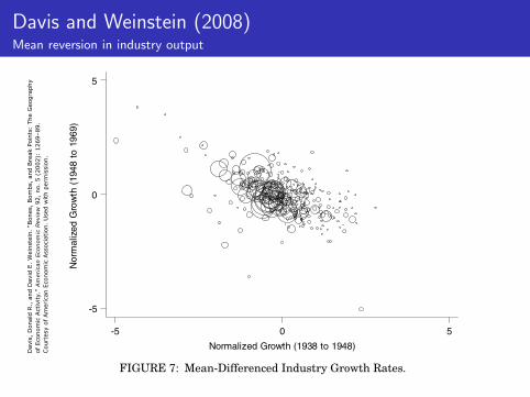
Davis and Weinstein (2008) Mean reversion in industry output DAVIS AND WEINSTEIN: A SEARCH FOR MULTIPLE EQUILIBRIA 53

Nor

mal

ized

Gro

wth

(19

48 t

o 19

69)

Normalized Growth (1938 to 1948)

-5 0 5

-5

0

5

FIGURE 7: Mean-Differenced Industry Growth Rates.

observations we find the same kind of mean reversion as Davis and Weinstein(2002, Figure 1) found in city population data.

Regression Results

In this section, we present our threshold regression results. Because it ispossible that multiple equilibria arise at one level of aggregation even if not atanother, we consider this at various levels of aggregation. We consider it firstusing the city population data considered in Davis and Weinstein (2002). Theanalysis of that data is augmented here by our new approach which sharpensthe contrast between the theory of unique versus multiple equilibria and whichalso places the theories on a more even footing in our estimation approach.Thereafter, we consider the same questions using data on city aggregate man-ufacturing and city-industry observations for eight manufacturing industries.Since manufacturing is less than half of all economic activity within a typicalcity, it should be clear that even if population in a city were to recover from theshocks, this need not be true of aggregate city-manufacturing. The same pointholds a fortiori for particular industries within manufacturing, which we alsoexamine.

We begin by considering city population data. Column 1 of Table 4 replicatesthe Davis and Weinstein (2002) results using population data. The IV estimatein column 1 tests a null of a unique stable equilibrium by asking if we can reject

C© Blackwell Publishing, Inc. 2008.

Dav

is,

Donal

d R

., a

nd D

avid

E.

Wei

nst

ein.

"Bones

, Bom

bs,

and B

reak

Poin

ts:

The

Geo

gra

phy

of

Eco

nom

ic A

ctiv

ity.

" Am

eric

an E

cono

mic

Rev

iew

92,

no.

5 (

2002):

1269–89.

Court

esy

of

Am

eric

an E

conom

ic A

ssoci

atio

n.

Use

d w

ith p

erm

issi

on.

Davis and Weinstein (2008) Mean reversion in industry output 54 JOURNAL OF REGIONAL SCIENCE, VOL. 48, NO. 1, 2008

Normalized Growth (1938 to 1948)

Ceramics

-4 -2 0 2-1

0

1

2

Chemicals

-1 0 1 2 3-2

-1

0

1

2

Processed Food

-2 -1 0 1 2-1

0

1

2

Lumber and Wood

-4 -2 0 2-6

-4

-2

2.2e-15

2

Machinery

-6 -4 -2 0 2-2

0

2

Metals

-4 -2 0 2

-1

0

1

2

3

Printing and Publishing

-4 -2 0 2

-2

-1

0

1

Textiles and Apparel

-4 -2 0 2-4

-2

0

2

4

FIGURE 8: Prewar vs Postwar Growth Rate.

that the coefficient on the wartime (1940–1947) growth rate is minus unity. Wecannot reject a coefficient of minus unity, hence cannot reject a null that there isa unique stable equilibrium. We also find that regionally-directed governmentreconstruction expenses following the war had no significant impact on citysizes 20 years after the war.

We next apply our threshold regression approach described above to testingfor multiple equilibria. This places unique and multiple equilibria on an evenfooting. The results are reported in the remaining columns of Table 4. In column2 of Table 4, we present the results for the estimation of equation (11) in the casein which there is a unique equilibrium. Given how close our previous estimateof � was to 0 (minus unity on wartime growth), it is not surprising that theestimates of the other parameters do not change much when we constrain � totake on this value.

Columns 3–5 present the results for threshold regressions premised onvarious numbers of equilibria.15 In these regressions, the constant plus �1 is

15In principle, we could have considered the possibility of more than four equilibria. However,neither the data plots nor any of the regression results suggested that raising the number ofpotential equilibria was likely to improve the results.

C© Blackwell Publishing, Inc. 2008.

Bleakley and Lin (2010) The ‘fall line’ is a geological feature. If one were traveling upstream from the ocean prior to the use of locks/canals, it the first point at which one would have had to engage in ‘portage’ (ie unload the boat and re-load a different boat upstream).

Appendix Figure A: The density of economic activity near intersections between the fall line and fall-line rivers

Notes: this map shows the contemporary distribution of economic activity across the southeastern U.S., measured by the 1996-7 nighttime lights layer from NationalAtlas.gov. The nighttimelights are used to present a nearly continuous measure of present-day economic activity at a high spatial frequency. The fall line (solid) is digitized from Physical Divisions of the United States,produced by the U.S. Geological Survey. Major rivers (dashed gray) are from NationalAtlas.gov, based on data produced by the U.S. Geological Survey. Many fall line-river intersections lie inpresent-day metropolitan areas, including (from the northeast) New Brunswick, Trenton, Philadelphia, Washington, Richmond, Fayetteville, Columbia, Augusta, Macon, Columbus, Tuscaloosa,Little Rock, Fort Worth, Austin, and San Antonio.

62

Courtesy of Jeffrey Lin and Hoyt Bleakley. Used with permission.

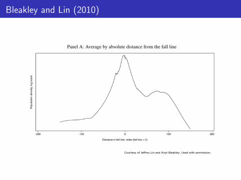
Bleakley and Lin (2010)

Panel A: Average by absolute distance from the fall line

Courtesy of Jeffrey Lin and Hoyt Bleakley. Used with permission.

MIT OpenCourseWare http://ocw.mit.edu

14.581 International Economics I Spring 2011

For information about citing these materials or our Terms of Use, visit: http://ocw.mit.edu/terms.

http://ocw.mit.edu/terms

http://ocw.mit.edu

Documents

14.581 lecture 10: Increasing returns to scale and … · —Lecture 10: Increasing Returns to Scale and Monopolistic Competition (Empirics) ... Bhagwati and Davis (1993) in a Chipman