Embed Size (px)
Citation preview

14.281 Contract Theory Notes
Richard HoldenMassachusetts Institute of Technology
E52-410Cambridge MA 02142
July 31, 2016
Contents
1 Introduction 41.1 Situating Contract Theory . . . . . . . . . . . . . . . . . . . . . . . . . . . . . 41.2 Types of Questions . . . . . . . . . . . . . . . . . . . . . . . . . . . . . . . . . 4
1.2.1 Insurance . . . . . . . . . . . . . . . . . . . . . . . . . . . . . . . . . . 41.2.2 Borrowing & Lending . . . . . . . . . . . . . . . . . . . . . . . . . . . 41.2.3 Relationship Specific Investments . . . . . . . . . . . . . . . . . . . . . 5
2 Mechanism Design 52.1 The Basic Problem . . . . . . . . . . . . . . . . . . . . . . . . . . . . . . . . . 62.2 Dominant Strategy Implementation . . . . . . . . . . . . . . . . . . . . . . . . 7
2.2.1 The Gibbard-Satterthwaite Theorem . . . . . . . . . . . . . . . . . . . 82.2.2 Quasi-Linear Preferences . . . . . . . . . . . . . . . . . . . . . . . . . 9
2.3 Bayesian Implementation . . . . . . . . . . . . . . . . . . . . . . . . . . . . . 112.4 Participation Constraints . . . . . . . . . . . . . . . . . . . . . . . . . . . . . 12
2.4.1 Public Project Example . . . . . . . . . . . . . . . . . . . . . . . . . . 132.4.2 Types of Participation Constraints . . . . . . . . . . . . . . . . . . . . 13
2.5 Optimal Bayesian Mechanisms . . . . . . . . . . . . . . . . . . . . . . . . . . 142.5.1 Welfare in Economies with Incomplete Information . . . . . . . . . . . 142.5.2 Durable Mechanisms . . . . . . . . . . . . . . . . . . . . . . . . . . . . 152.5.3 Robust Mechanism Design . . . . . . . . . . . . . . . . . . . . . . . . . 19
3 Adverse Selection (Hidden Information) 203.1 Static Screening . . . . . . . . . . . . . . . . . . . . . . . . . . . . . . . . . . . 20
3.1.1 Introduction . . . . . . . . . . . . . . . . . . . . . . . . . . . . . . . . 203.1.2 Optimal Income Tax . . . . . . . . . . . . . . . . . . . . . . . . . . . . 243.1.3 Regulation . . . . . . . . . . . . . . . . . . . . . . . . . . . . . . . . . 263.1.4 The General Case – n types and a continnum of types . . . . . . . . . 283.1.5 Random Schemes . . . . . . . . . . . . . . . . . . . . . . . . . . . . . . 323.1.6 Extensions and Applications . . . . . . . . . . . . . . . . . . . . . . . 33
3.2 Dynamic Screening . . . . . . . . . . . . . . . . . . . . . . . . . . . . . . . . . 34
1

3.2.1 Durable good monopoly . . . . . . . . . . . . . . . . . . . . . . . . . . 343.2.2 Non-Durable Goods . . . . . . . . . . . . . . . . . . . . . . . . . . . . 383.2.3 Soft Budget Constraint . . . . . . . . . . . . . . . . . . . . . . . . . . 39
4 Moral Hazard 404.1 Introduction . . . . . . . . . . . . . . . . . . . . . . . . . . . . . . . . . . . . . 404.2 The Basic Principal-Agent Problem . . . . . . . . . . . . . . . . . . . . . . . . 40
4.2.1 A Fairly General Model . . . . . . . . . . . . . . . . . . . . . . . . . . 404.2.2 The First-Order Approach . . . . . . . . . . . . . . . . . . . . . . . . . 414.2.3 Beyond the First-Order Approach I: Grossman-Hart . . . . . . . . . . 434.2.4 Beyond the First-Order Approach II: Holden (2005) . . . . . . . . . . 464.2.5 Value of Information . . . . . . . . . . . . . . . . . . . . . . . . . . . . 524.2.6 Random Schemes . . . . . . . . . . . . . . . . . . . . . . . . . . . . . . 534.2.7 Linear Contracts . . . . . . . . . . . . . . . . . . . . . . . . . . . . . . 54
4.3 Multi-Agent Moral Hazard . . . . . . . . . . . . . . . . . . . . . . . . . . . . 574.3.1 Relative Performance Evaluation . . . . . . . . . . . . . . . . . . . . . 574.3.2 Moral Hazard in Teams . . . . . . . . . . . . . . . . . . . . . . . . . . 594.3.3 Random Schemes . . . . . . . . . . . . . . . . . . . . . . . . . . . . . . 604.3.4 Tournaments . . . . . . . . . . . . . . . . . . . . . . . . . . . . . . . . 614.3.5 Supervision & Collusion . . . . . . . . . . . . . . . . . . . . . . . . . . 644.3.6 Hierarchies . . . . . . . . . . . . . . . . . . . . . . . . . . . . . . . . . 65
4.4 Moral Hazard with Multiple Tasks . . . . . . . . . . . . . . . . . . . . . . . . 684.4.1 Holmstrom-Milgrom . . . . . . . . . . . . . . . . . . . . . . . . . . . . 68
4.5 Dynamic Moral Hazard . . . . . . . . . . . . . . . . . . . . . . . . . . . . . . 704.5.1 Stationarity and Linearity of Contracts . . . . . . . . . . . . . . . . . 704.5.2 Renegotiation . . . . . . . . . . . . . . . . . . . . . . . . . . . . . . . . 74
4.6 Relational Contracts and Career Concerns . . . . . . . . . . . . . . . . . . . . 764.6.1 Career Concerns . . . . . . . . . . . . . . . . . . . . . . . . . . . . . . 764.6.2 Multi-task with Career Concerns . . . . . . . . . . . . . . . . . . . . . 794.6.3 Relational Contracts . . . . . . . . . . . . . . . . . . . . . . . . . . . . 80
5 Incomplete Contracts 845.1 Introduction and History . . . . . . . . . . . . . . . . . . . . . . . . . . . . . 845.2 The Hold-Up Problem . . . . . . . . . . . . . . . . . . . . . . . . . . . . . . . 85
5.2.1 Solutions to the Hold-Up Problem . . . . . . . . . . . . . . . . . . . . 875.3 Formal Model of Asset Ownership . . . . . . . . . . . . . . . . . . . . . . . . 87
5.3.1 Different Bargaining Structures . . . . . . . . . . . . . . . . . . . . . . 915.3.2 Empirical Work . . . . . . . . . . . . . . . . . . . . . . . . . . . . . . . 915.3.3 Real versus Formal Authority . . . . . . . . . . . . . . . . . . . . . . . 92
5.4 Financial Contracting . . . . . . . . . . . . . . . . . . . . . . . . . . . . . . . 945.4.1 Incomplete Contracts & Allocation of Control . . . . . . . . . . . . . . 945.4.2 Costly State Verification . . . . . . . . . . . . . . . . . . . . . . . . . . 965.4.3 Voting Rights . . . . . . . . . . . . . . . . . . . . . . . . . . . . . . . . 985.4.4 Collateral and Maturity Structure . . . . . . . . . . . . . . . . . . . . 100
5.5 Public v. Private Ownership . . . . . . . . . . . . . . . . . . . . . . . . . . . 1035.6 Markets and Contracts . . . . . . . . . . . . . . . . . . . . . . . . . . . . . . . 106
5.6.1 Overview . . . . . . . . . . . . . . . . . . . . . . . . . . . . . . . . . . 1065.6.2 Contracts as a Barier to Entry . . . . . . . . . . . . . . . . . . . . . . 107
2

5.6.3 Product Market Competition and the Principal-Agent Problem . . . . 1095.7 Foundations of Incomplete Contracts . . . . . . . . . . . . . . . . . . . . . . . 112
5.7.1 Implementation Literature . . . . . . . . . . . . . . . . . . . . . . . . . 1135.7.2 The Hold-Up Problem . . . . . . . . . . . . . . . . . . . . . . . . . . . 116
3

1 Introduction
1.1 Situating Contract Theory
Think of (at least) three types of modelling environments
1. Competitive Markets: Large number of players → General Equilibrium Theory
2. Strategic Situations: Small number of players → Game Theory
3. Small numbers with design → Contract Theory & Mechanism Design
• Don’t take the game as given
• Tools for understanding institutions
1.2 Types of Questions
1.2.1 Insurance
• 2 parties A & B
• A faces risk - say over income YA = 0, 100, 200 with probabilities1/3, 1/3, 1/3 and is risk-averse
• B is risk-neutral
• Gains from trade
• If A had all the bargaining power the risk-sharing contract is B pays A 100
• But we don’t usually see full insurance in the real world
1. Moral Hazard (A can influence the probabilities)
2. Adverse Selection (There is a population of A’s with different probabilities &only they know their type)
1.2.2 Borrowing & Lending
• 2 players
• A has a project, B has money
• Gains from trade
• Say return is f(e, θ) where e is effort and θ is the state of the world
• B only sees f not e or θ
• Residual claimancy doesn’t work because of limited liability (could also have risk-aversion)
• No way to avoid the risk-return trade-off
4

1.2.3 Relationship Specific Investments
• A is an electricity generating plant (which is movable pre hoc)
• B is a coal mine (immovable)
• If A locates close to B (to save transportation costs) they make themselves vulnerable
• Say plant costs 100
• “Tomorrow” revenue is 180 if they get coal, 0 otherwise
• B’s cost of supply is 20
• Zero interest rate
• NPV is 180-20-100=60
• Say the parties were naive and just went into period 2 cold
• Simple Nash Bargaining leads to a price of 100
• πA = (180− 100)− 100 = −20
• An illustration of the Hold-Up Problem
• Could write a long-term contract: bounded between 20 and 80 due to zero profit pricesfor A & B, maybe it would be 50
• But what is contract are incomplete – the optimal contract may be closer to no contractthan a very fully specified one
• Maybe they should merge?
2 Mechanism Design
• Often, individual preferences need to be aggregated
• But if preferences are private information then individuals must be relied upon toreveal their preferences
• What constraints does this place on social decisions?
• Applications:
– Voting procedures
– Design of public institutions
– Writing of contracts
– Auctions
5
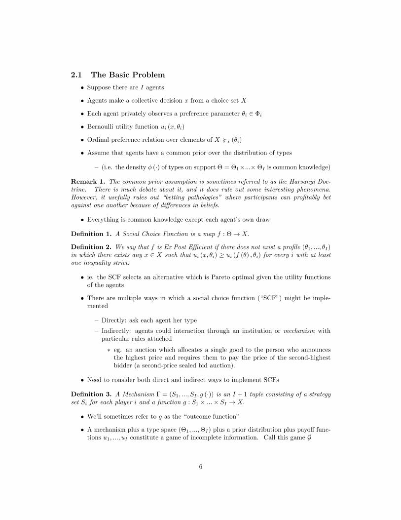
2.1 The Basic Problem
• Suppose there are I agents
• Agents make a collective decision x from a choice set X
• Each agent privately observes a preference parameter θi ∈ Φi
• Bernoulli utility function ui (x, θi)
• Ordinal preference relation over elements of X <i (θi)
• Assume that agents have a common prior over the distribution of types
– (i.e. the density φ (·) of types on support Θ = Θ1×...× ΘI is common knowledge)
Remark 1. The common prior assumption is sometimes referred to as the Harsanyi Doc-trine. There is much debate about it, and it does rule out some interesting phenomena.However, it usefully rules out “betting pathologies” where participants can profitably betagainst one another because of differences in beliefs.
• Everything is common knowledge except each agent’s own draw
Definition 1. A Social Choice Function is a map f : Θ→ X.
Definition 2. We say that f is Ex Post Efficient if there does not exist a profile (θ1, ..., θI)in which there exists any x ∈ X such that ui (x, θi) ≥ ui (f (θ) , θi) for every i with at leastone inequality strict.
• ie. the SCF selects an alternative which is Pareto optimal given the utility functionsof the agents
• There are multiple ways in which a social choice function (“SCF”) might be imple-mented
– Directly: ask each agent her type
– Indirectly: agents could interaction through an institution or mechanism withparticular rules attached
∗ eg. an auction which allocates a single good to the person who announcesthe highest price and requires them to pay the price of the second-highestbidder (a second-price sealed bid auction).
• Need to consider both direct and indirect ways to implement SCFs
Definition 3. A Mechanism Γ = (S1, ..., SI , g (·)) is an I + 1 tuple consisting of a strategyset Si for each player i and a function g : S1 × ...× SI → X.
• We’ll sometimes refer to g as the “outcome function”
• A mechanism plus a type space (Θ1, ...,ΘI) plus a prior distribution plus payoff func-tions u1, ..., uI constitute a game of incomplete information. Call this game G
6

Remark 2. This is a normal form representation. At the end of the course we will considerusing an extensive form when we study subgame perfect implementation.
• In a first-price sealed-bid auction Si = R+ and given bids b1, ..., bI the outcome func-
tion g (b1, ..., bI) =({yi (b1, ..., bI)}Ii=1 , {ti (b1, ..., bI)}Ii=1
)such that yi (b1, ..., bI) = 1
iff i = min {j : bj = max {b1, ..., bI}} and ti (b1, ..., bI) = −biyi (b1, ..., bI)
Definition 4. A strategy for player i is a function si : Θi → Si.
Definition 5. The mechanism Γ is said to Implement a SCF f if there exists equilibriumstrategies (s∗1 (θ1) , ..., s∗I (θI)) of the game G such that g (s∗1 (θ1) , ..., s∗I (θI)) = f (θ1, ..., θI)for all (θ1, ..., θI) ∈ Θ1 × ...×ΘI .
• Loosely speaking: there’s an equilibrium of G which yields the same outcomes as theSCF f for all possible profiles of types.
• We want it to be true no matter what the actual types (ie. draws) are
Remark 3. We are requiring only an equilibrium, not a unique equilibrium.
Remark 4. We have not specified a solution concept for the game. The literature hasfocused on two solution concepts in particular: dominant strategy equilibrium and BayesNash equilibrium.
• The set of all possible mechanisms is enormous!
• The Revelation Principle provides conditions under which there is no loss of generalityin restricting attention to direct mechanisms in which agents truthfully reveal theirtypes in equilibrium.
Definition 6. A Direct Revelation Mechanism is a mechanism in which Si = Θi for all iand g (θ) = f (θ) for all θ ∈ (Θ1 × ...×ΘI) .
Definition 7. The SCF f is Incentive Compatible if the direct revelation mechanism Γ hasan equilibrium (s∗1 (θ1) , ..., s∗I (θI)) in which s∗i (θi) = θi for all θi ∈ Θi and all i.
2.2 Dominant Strategy Implementation
• A strategy for a player is weakly dominant if it gives her at least as high a payoff asany other strategy for all strategies of all opponents.
Definition 8. A mechanism Γ Implements the SCF f in dominant strategies if there existsa dominant strategy equilibrium of Γ, s∗ (·) = (s∗1 (·) , ..., s∗I (·)) such that g (s∗ (θ)) = f (θ)for all θ ∈ Θ.
• A strong notion, but a robust one
– eg. don’t need to worry about higher order beliefs
– Doesn’t matter if agents miscalculate the conditional distribution of types
– Works for any prior distribution φ (·) so the mechanism designer doesn’t need toknow this distribution
7

Definition 9. The SCF f is Truthfully Implementable in Dominant Strategies if s∗i (θi) = θifor all θi ∈ Θi and i = 1, ..., I is a dominant strategy equilibrium of the direct revelationmechanism Γ = (Θ1, ...,ΘI , f (·)) , ie
ui (f (θi, θ−i) , θi) ≥ ui(f(θi, θ−i
), θi
)for all θi ∈ Θi and θ−i ∈ Θ−i. (1)
Remark 5. This is sometimes referred to as being “dominant strategy incentive compatible”or “strategy-proof”.
Remark 6. The fact that we can restrict attention without loss of generality to whetherf (·) in incentive compatible is known as the Revelation Principle (for dominant strategies).
• This is very helpful because instead of searching over a very large space we only haveto check each of the inequalities in (1).
– Although we will see that this can be complicated (eg. when there are an un-countably infinite number of them).
Theorem 1. (Revelation Principle for Dominant Strategies) Suppose there exists a mecha-nism Γ that implements the SCF f in dominant strategies. Then f is incentive compatible.
Proof. The fact that Γ implements f in dominant strategies implies that there exists s∗ (·) =(s∗1 (·) , ..., s∗I (·)) such that g (s∗ (θ)) = f (θ) for all θ and that, for all i and θi ∈ Θi, we have
ui (g (s∗i (θi) , s−i) , θi) ≥ ui (g (si (θi) , s−i) , θi) for all si ∈ Si, s−i ∈ S−i.
In particular, this means that for all i and θi ∈ Θi
ui(g(s∗i (θi) , s
∗−i (θ−i)
), θi)≥ ui
(g(s∗i
(θi
), s∗−i (θ−i)
), θi
),
for all θi ∈ Θi, θ−i ∈ Θ−i. Since g (s∗ (θ)) = f (θ) for all θ, the above inequality impliesthat for all i and θi ∈ Θi
ui (f (θi, θ−i) , θi) ≥ ui(f(θi, θ−i
), θi
)for all θi ∈ Θi, θ−i ∈ Θ−i,
which is precisely incentive compatibility.
• Intuition: suppose there is an indirect mechanism which implements f in dominantstrategies and where agent i plays strategy s∗i (θi) when she is type θi. Now supposewe asked each agent her type and played s∗i (θi) on her behalf. Since it was a dominantstrategy it must be that she will truthfully announce her type.
2.2.1 The Gibbard-Satterthwaite Theorem
Notation 1. Let P be the set of all rational preference relations < on X where there is noindifference
Notation 2. Agent i’s set of possible ordinal preference relations on X are denoted Ri ={<i:<i=<i (θi) for some θi ∈ Θi}
Notation 3. Let f (Θ) = (x ∈ X : f(θ) = x for some θ ∈ Θ) be the image of f (·) .
8

Definition 10. The SCF f is Dictatorial if there exists an agent i such that for all θ ∈ Θwe have:
f (θ) ∈ {x ∈ X : ui (xi, θi) ≥ ui (y, θi) ,∀y ∈ X} .
• Loosely: there is some agent who always gets her most preferred alternative under f.
Theorem 2. (Gibbard-Satterthwaite) Suppose: (i) X is finite and contains at least threeelements, (ii) Ri = P for all i, and (iii) f (Θ) = X. Then the SCF f is dominant strategyimplementable if and only if f is dictatorial.
Remark 7. Key assumptions are that individual preferences have unlimited domain andthat the SCF takes all values in X.
• The idea of a proof is the following: identify the pivotal voter and then show that sheis a dictator
– See Benoit (Econ Lett, 2003) proof
– Very similar to Geanakoplos (Cowles, 1995) proof of Arrow’s Impossibility The-orem
– See Reny paper on the relationship
• This is a somewhat depressing conclusion: for a wide class of problems dominantstrategy implementation is not possible unless the SCF is dictatorial
• It’s a theorem, so there are only two things to do:
– Weaken the notion of equilibrium (eg. focus on Bayes Nash equilibrium)
– Consider more restricted environments
• We begin by focusing on the latter
2.2.2 Quasi-Linear Preferences
• An alternative from the social choice set is now a vector x = (k, t1, ..., tI), where k ∈ K(with K finite) is a choice of “project”.
• ti ∈ R is a monetary transfer to agent i
• Agent i’s preferences are represented by the utility function
ui(x, θ) = vi (k, θi) + (mi + ti) ,
where mi is her endowment of money.
• Assume no outside parties
• Set of alternatives is:
X =
{(k, t1, ..., tI) : k ∈ K, ti ∈ R for all i and
∑i
ti ≤ 0
}.
9

• Now consider the following mechanism: agent i receives a transfer which depends onhow her announcement of type affects the other agent’s payoffs through the choice ofproject. Specifically, agent i’s transfer is exactly the externality that she imposes onthe other agents.
• A SCF is ex post efficient in this environment if and only if:
I∑i=1
vi (k (θ) , θi) ≥I∑i=1
vi (k, θi) for all k ∈ K, θ ∈ Θ, k (θ) .
Proposition 1. Let k∗ (·) be a function which is ex post efficient. The SCF f = (k∗ (·) , t1, ..., tI)is truthfully implementable in dominant strategies if, for all i = 1, ..., I
ti (θ) =
∑j 6=i
vj (k∗ (θ) , θj)
+ hi (θ−i) , (2)
where hi is an arbitrary function.
• This is known as a Groves-Clarke mechanism
Remark 8. Technically this is actually a Groves mechanism after Groves (1973). Clarke(1971) discovered a special case of it where the transfer made by an agent is equal to theexternality imposed on other agent’s if she is pivotal, and zero otherwise.
• Groves-Clarke type mechanisms are implementable in a quasi-linear environment
• Are these the only such mechanisms which are?
• Green and Laffont (1979) provide conditions under which this question is answered inthe affirmative
• Let V be the set of all functions v : K → R
Theorem 3. (Green and Laffont, 1979) Suppose that for each agent i = 1, ..., I we have{vi (·, θi) : θi ∈ Θi} = V. Then a SCF f = (k∗ (·) , t1 (·) , ..., tI (·)) in which k∗ (·) satisfies
I∑i=1
vi (k (θ) , θi) ≥I∑i=1
vi (k, θi) ,
for all k ∈ K (efficient project choice) is truthfully implementable in dominant strategiesonly if ti (·) satisfies (2) for all i = 1, ..., I.
• ie. if every possible valuation function from K to R arises for some type then a SCFwhich is truthfully implementable must be done so through a mechanism in the Grovesclass
• So far we have focused on only one aspect of ex post efficient efficiency–that theefficient project be chosen
• Another requirement is that none of the numeraire be wasted
10

• The condition is sometimes referred to as “budget balance” and requires∑i
ti (θ) = 0 for all θ ∈ Θ.
• Can we satisfy both requirements?
• Green and Laffont (1979) provide conditions under which this question is answered inthe negative
Theorem 4. (Green and Laffont, 1979) Suppose that for each agent i = 1, ..., I we have{vi (·, θi) : θi ∈ Θi} = V. Then there does not exists a SCF f = (k∗ (·) , t1 (·) , ..., tI (·)) inwhich k∗ (·) satisfies
I∑i=1
vi (k (θ) , θi) ≥I∑i=1
vi (k, θi) ,
for all k ∈ K (efficient project choice) and∑i
ti (θ) = 0 for all θ ∈ Θ,
(budget balance).
• Either have to waste some of the numeraire or give up on efficient project choice
• Can get around this if there is one agent whose preferences are known
– Maybe one agent doesn’t care about project choice
– eg. the seller in an auction
– Maybe the project only affects a subset of the population...
• Need to set the transfer for the “no private information” type to tBB (θ) = −∑i 6=0 ti (θ)
for all θ.
• This agent is sometime referred to as the “budget breaker”
• We will return to this theme later in the course (stay tuned for Legros-Matthews)
2.3 Bayesian Implementation
• Now move from dominant strategy equilibrium as the solution concept to Bayes-Nashequilibrium
• A strategy profile implements an SCF f in Bayes-Nash equilibrium if for all i and allθi ∈ Θi we have
Eθ−i[ui(g(s∗i (θi) , s
∗−i (θ−i)
), θi)|θi]≥
Eθ−i[ui(g(si (θi) , s
∗−i (θ−i)
), θi)|θi],
for all si ∈ Si.
11

• Again, we are able to make use of the revelation principle
• Same logic as in dominant strategy case
– If an agent is optimizing by choosing s∗i (θi) in some mechanism Γ then if weintroduce an intermediary who will play that strategy for her then telling thetruth is optimal conditional on other agents doing so. So truth telling is a(Bayes-Nash) equilibrium of the direct revelation game (ie. the one with theintermediary).
Remark 9. Bayesian implementation is a weaker notion than dominant strategy implemen-tation. Every dominant strategy equilibrium is a Bayes-Nash equilibrium but the converseis false. So any SCF which is implementable in dominant strategies can be implemented inBayes-Nash equilibrium, but not the converse.
Remark 10. Bayesian implementation requires that truth telling give the highest payoff av-eraging over all possible types of other agents. Dominant strategy implementation requiresthat truth telling be best for every possible type of other agent.
• Can this relaxation help us overcome the negative results of dominant strategy imple-mentation
• Again consider a quasi-linear environment
• Under the conditions of Green-Laffont we couldn’t implement a SCF truthfully andhave efficient project choice and budget balance
• Can we do better in Bayes-Nash?
• A direct revelation mechanism known as the “expected externality mechanism” due tod’Aspremont and Gerard-Varet (1979) and Arrow (1979) answers this in the affirmative
• Under this mechanism the transfers are given by:
ti (θ) = Eθ−i
∑j 6=i
vj
(k∗(θi, θ−i
), θj
)+ hi (θ−i) .
• The first term is the expected benefit of other agents when agent i announces her typeto be θi and the other agents are telling the truth
2.4 Participation Constraints
• So far we have worried a lot about incentive compatibility
• But we have been assuming that agents have to participate in the mechanism
• What happens if participation is voluntary?
12

2.4.1 Public Project Example
• Decision to do a project or not K = {0, 1}
• Two agents with Θi = {L,H} being the (real-valued) valuations of the project
• Assume that H > 2L > 0
• Cost of project is c ∈ (2L,H)
• An ex post efficient SCF has k∗ (θ1, θ2) = 1 if either θ1 = H or θ2 = H and k∗ (θ1, θ2) =0 if (and only if) θ1 = θ2 = L
• With no participation constraint we can implement this SCF in dominant strategiesusing a Groves scheme
• By voluntary participation we mean that an agent can withdraw at any time (and ifso, does not get any of the benefits of the project)
• With voluntary participation agent 1 must have t1 (L,H) ≥ −L
– Can’t have to pay more than L when she values the project at L because won’tparticipate voluntarily
• Suppose both agents announce H. For truth telling to be a dominant strategy weneed:
Hk∗ (H,H) + t1(H,H) ≥ Hk∗ (L,H) + t1(L,H)
H + t1(H,H) ≥ H + t1(L,H)
t1(H,H) ≥ t1(L,H)
• But we know that t1 (L,H) ≥ −L, so t1(H,H) ≥ −L
• Symmetrically, t2(H,H) ≥ −L
• So t1 (L,H) + t2(H,H) ≥ −2L
• But since c > 2L we can’t satisfy t1 (L,H) + t2(H,H) ≥ −c
• Budget breaker doesn’t help either, because tBB (θ1, θ2) ≥ 0 for all (θ1, θ2) and hencet0 (H,H) ≥ 0 and we can’t satisfy
t0(H,H) + t1(H,H) + t2(H,H) ≤ −c.
2.4.2 Types of Participation Constraints
• Distinguish between three different types of participation constraint depending ontiming (of when agents can opt out of the mechanism)
• Ex ante: before the agents learn their types, ie:
Ui(f) ≥ Eθi [ui (θi)] . (3)
13

• Interim: after agents know their own types but before the take actions (under themechanism), ie:
Ui(θ|f) = Eθ−i [ui (f (θi, θ−i) , θi) |θi] ≥ ui (θi) for all θi. (4)
• Ex post: after types have been announced and an outcome has been chosen (it’s adirect revelation mechanism)
ui (f (θi, θ−i) , θi) ≥ ui (θi) for all (θi, θ−i) (5)
• A question of when agents can agree to be bound by the mechanism
• Constraints are most severe when agents can withdraw ex post and least severe whenthey can withdraw ex ante. This can be seen from the fact that (5)⇒(4)⇒(3) butthe converse doesn’t hold
Theorem 5. (Myerson-Satterthwaite) Suppose there is a risk-neutral seller and risk-neutralbuyer of an indivisible good and suppose their respective valuations are drawn from [θ1, θ1] ∈R and [θ2, θ2] ∈ R according to strictly positive densities with (θ1, θ1) ∩ (θ2, θ2) 6= ∅. Thenthere does not exist a Bayesian incentive compatible SCF which is ex post efficient and givesevery type non-negative expected gains from participation.
• Whenever gains from trade are possible but not certain there is no ex post efficientSCF which is incentive compatible and satisfies interim participation constraints
Remark 11. This applies to all voluntary trading institutions, including all bargainingprocesses.
2.5 Optimal Bayesian Mechanisms
2.5.1 Welfare in Economies with Incomplete Information
• We have been concerned thus far with which SCFs are implementable
• We turn to evaluation of different implementable SCFs
• Want to be able to evaluate different “decision rules” or mechanisms
• Need to extend the notion of Pareto optimality where agents’ preference are not knownwith certainty
• Pareto: “A decision rule is efficient if and only if no other feasible decision rule canbe found that makes some individual better-off without making any worse-off”
• Need a notion of: (i) a feasible SCF, (ii) know what better-off means in this context,and (iii) specify who’s doing the finding
• Feasibility: Bayesian incentive compatible plus individually rational
• Call this set the “incentive feasible set” F ∗ (Myerson, 1991)
• Better-off: depends on the timing
14

– Before agents learn their types: ex ante efficiency
– After agents learn their types: interim efficiency
• Putting (i) and (ii) together we refer to “ex ante incentive efficiency” and “interimincentive efficiency” (Holmstrom and Myerson, 1983)
• These are different from our previous definition of ex post efficiency
• Here that would require evaluation of SCFs after all information has been revealed
• The two definitions are equivalent if and only if F = {f : Θ→ X}
• Who’s doing the finding? Outside planner or the informed individuals within theeconomy
• Basic notion: the economist is an outside observer
– Can’t predict what decision or allocation will prevail without having all the pri-vate information
• With incomplete information the informed individuals might be able to agree (unani-mously) to change a decision rule which a planner could not identify as an improvement
2.5.2 Durable Mechanisms
• Holmstrom-Myerson (Ecta, 1983)
• Suppose a mechanism M is interim incentive efficient
• A social planner can’t propose another incentive-compatible decision rule which evertype is sure to prefer to M
• But it could be that there exists another mechanism M ′ such that:
ui (M ′|θi) > ui (M |θi) for all i.
• So if the types were θ1, ..., θI then all agents would prefer M to M ′
• Are we done?
• Not even nearly
• Suppose agent 2 announces that she prefers M ′ to M, then agent 1 might want to saythat she prefers M to M ′
– Agent 2 has revealed some new information to agent 1
• If agents unanimously agreed to change from M to M ′ then it would be commonknowledge that all individuals prefer M ′ to M
• Recall Aumann (1976): If agents have a common prior and their posteriors are commonknowledge then those posteriors must be equal
• Recall also the “no-trade theorems” (see Milgrom and Stokey, JET, 1982)
15

– Milgrom-Stokey provide conditions under which Nash equilibrium and commonknowledge that all players have prefer the proposed allocation to the initial one
– Common prior and risk-neutrality
– No trade based solely because of differences in beliefs.
• Denote agent i’s prior as πi
Definition 11. An event R is Common Knowledge if and only if R = R1 × ... × RI withRi ⊆ Θi for all i and
πi
(θ−i|θi
)= 0,
for all θi ∈ R, θ−i 6∈ R and for i.
• ie, the information state R of the economy is common knowledge iff all individualsassign zero probability to events outside R
Definition 12. We say that M ′ Interim Dominates M within R if and only if R 6= ∅ and
ui (M ′|θi) ≥ ui (M |θi) ,
for all θ ∈ R, for all i, with at least one inequality strict.
• If M is incentive efficient and each agent knows her own type then it can’t be commonknowledge that the agents unanimously prefer another mechanism M ′
Theorem 6. (Holmstrom-Myerson) An incentive compatible mechanism M is interimincentive efficient if and only if there does not exist any event R which is common-knowledgesuch that M is interim dominated within R by another incentive-compatible mechanism.
• Doesn’t mean they couldn’t unanimously agree to move to another incentive efficientmechanism M ′
– But if unanimous agreement is reached then every agent must know more thanher own type
– ie, there must have been communication
• Now want to ask the following question: if a mechanism is determined by the agentsthemselves, after their types are privately observed, what are the properties of therules which will emerge?
• We will be interested in durable mechanisms
– ie. mechanisms which the agents will never unanimously agree to change
An example
• Suppose there are two agents: 1 and 2
• Each agent can be type a or b
• So there are four possible combinations of types
16

• Assume that each are ex ante equally likely
• Decision from the set {A,B,C}
• Payoffs (vNM)
u1a u1b u2a u2b
A 2 0 2 2B 1 4 1 1C 0 9 0 −8
• Note: sticking with the assumption that payoffs depend only on own type
• Note that agent 2, when of either type, prefers A to B and B to C
• So does agent 1a
• Agent 1b prefers C to B to A
• The following incentive compatible mechanism maximizes the sum of utilities (amongIC mechanisms)
M (1a, 2a) = A
M(1b, 2a) = C
M(1a, 2b) = B
M(1b, 2b) = B
• This mechanism selects C is the types are 1b and 2a
• It selects B if the types are 1b and 2b
• Note that 2a can ensure either A or C by reporting truthfully, or ensure B by lying
• Since agent 2 has a 50-50 prior over agent 1 being type a or b she gets the sameexpected utility from reporting truthfully and lying
– So we presume that she reports truthfully
• M is both ex ante and interim incentive efficient
– So no planner could come up with a better mechanism
• Now suppose agent 1 is type 1a
• Knowing this, she knows that both she and agent 2 prefer A to what the mechanismwill give rise to
– And if she proposed that they choose A then agent 2 would be happy to acceptthat
• So, M is incentive efficient but there’s an improvement to be made
– The deterministic mechanism M ′ (·, ·) = A
17

• Now suppose that agent 1 insists of using M rather than changing to choice A
– Agent 2 would know that agent 1 was 1b
– Now M isn’t incentive compatible because both 2a and 2b would announce 2band ensure B (rather than announce 2a and get C)
• Conclusion: if agents already know their types then M could not be implemented eventhough it is incentive compatible and incentive efficient
– It’s not durable
Existence
• Do durable mechanisms exist?
Definition 13. We say that an incentive compatible mechanism M is “Uniformly IncentiveCompatible” if and only if
ui (M (θ) , θ) ≥ ui(M(θ−i, θi
), θ),
for all i, for all θ ∈ Θ and for all θi ∈ Θi.
• ie. no individual would ever want to lie under the mechanism, even if she knew theother agents’ types, assuming that they were going to report truthfully
• This is now usually called “ex post incentive compatibility”
Theorem 7. Suppose a mechanism M if uniformly incentive compatible and interim in-centive efficient. Then M is durable.
• The main (and encouraging) result is the following
Theorem 8. There exists a nonempty set of decision rules that are both durable and incen-tive efficient
• Are there decision rules that are durable but not incentive efficient?
• Sure
• Suppose the same type structure as above, but now two possible decisions A and B
• Preferences
u1 (A, θ) = u2 (A, θ) = 2 for all θ
u1 (B, θ) = u1 (B, θ) = 3 if θ = (1a, 2a) or (1b, 2b)
u1 (B, θ) = u1 (B, θ) = 0 if θ = (1a, 2b) or (1b, 2a)
• Consider the deterministic mechanism M which always selects A
• M is not interim incentive efficient but it is durable
– Would be better to do B when the types match
– But with any alternative mechanism there is an equilibrium in which there arereports which are independent of θ
18

2.5.3 Robust Mechanism Design
• Bergemann and Morris (Ecta, 2005)
• A key assumption in all that we have done so far is that the mechanism designer knowsthe prior distribution π
• Harsanyi’s important idea: an agent’s type should include beliefs about the strategicenvironment, beliefs about other players beliefs, ...
– A sufficiently rich type space can then describe any environment
– This is sometimes called the implicit approach to modelling higher order beliefs(see Heifetz and Samet, JME 1999 for further details)
• With a sufficiently rich type space it is a tautology that there is common knowledgeof each agent’s set of types and beliefs about other agents’ types
• This notion is formalized in the universal type space of Mertens and Zamir (1985) (seealso Brandenburdger and Dekel, 1993)
• If we assume a smaller type space and still maintain the assumption of common knowl-edge then the model may not be internally consistent
• What happens to Bayesian implementation without a common prior?
• Bergemann-Morris refer to this as interim implementation
• We have focused thus far on payoff type spaces
• But there many be many types of an agent who share the same payoff type
– eg. they have different higher order beliefs
– These are (much) smaller than the universal type space
• What we have done up until now is work with a very small type space (the payofftype space) and then assume that all agents (including the planner) have a commonknowledge prior over that type space
• The largest type space we could work with is the union of all possible type space thatcould have arisen from the payoff environment
– This is equivalent to the universal type space
• The paper also considers environments where there are both private values and com-mon values
Definition 14. An environment is said to be Separable if there exists ui : X0×...×XI×Θ→R such that
ui ((x0, x1, ..., xI) , θ) = ui (x0, xi, θ)
for all i, x ∈ X and θ ∈ Θ; and there exists a function f0 : Θ→ X0 and, for each agent i, anonempty valued correspondence Fi : Θ→ 2Xi/∅ such that
F (θ) = f0 (θ)× F1 (θ)× ...× FI (θ) .
19

• The bite comes from the implication that the set of permissible private componentsfor any agent does not depend on the choice of the private component for the otheragents
• Quasi-linear environments with no restrictions on transfers (eg. don’t require budgetbalance) are special cases of separable environments
• So are environments where utility depends only on the common component and payofftype profile θ
Remark 12. Any SCF is separable. It is only social choice correspondences which maynot be separable
• BM show that there can be social choice correspondences which are interim imple-mentable on all payoff type spaces but not interim implementable on all type spaces
• They also show that in separable environments all of the following statements areequivalent for a social choice correspondence F
– F is interim implementable on all type spaces
– F is interim implementable on all common prior type spaces
– F is interim implementable on all payoff type spaces
– F is interim implementable on all common prior payoff type spaces
– F is ex post implementable
3 Adverse Selection (Hidden Information)
3.1 Static Screening
3.1.1 Introduction
• A good reference for further reading is Fudenberg & Tirole chapter 7
• Different to “normal” Adverse Selection because 1 on 1, not a market setting
• 2 players: Principal and the Agent
• Payoff: Agent G (u (q, θ)− T ), Principal H (v (q, θ) + T ) where G (·) , H (·) are concavefunctions and q is some verifiable outcome (eg. output), T is a transfer, θ is the Agent’sprivate information
• Don’t use the concave transforms for now
• Say Principal is a monopolistic seller and the Agent is a consumer
• Let v(q, θ) = −cq
• Principal’s payoff is T − cq where T is total payment (pq)
• u(q, θ) = θV (q)
20

• Agent’s payoff is θV (q)− T where V (·) is strictly concave
• θ is type (higher θ → more benefit from consumption)
• θ = θ1, ..., θn with probabilities p1, ..., pn
• Principal only knows the distribution of types
• Note: relationship to non-linear pricing literature
• Assume that the Principal has all the bargaining power
• Start by looking at the first-best outcome (ie. under symmetric information)
First Best Case I: Ex ante no-one knows θ, ex post θ is verifiable
• Principal solves
max(qi,Ti)
n
i=1
pi(Ti − cqi)
s.t.ni=1pi(θiV (qi)− Ti) ≥ U (PC)
First Best Case II: Ex ante both know θ
• Normalize U to 0
• Principal solves
max(qi,Ti)
{Ti − cqi}
s.t.θiV (qi)− T ≥ 0 (PC)
• The PC will bind, so Ti = θiV (qi)
• So they just solve maxqi{θiV (qi)− cqi}
• FOC θiV′(qi) = c
• This is just perfect price discrimination – efficient but the consumer does badly
• Case I folds into II by offering a contingent contract
21

Second-Best
• Agent knows θi but the Principal doesn’t
• First ask if we can achieve/sustain the first best outcome
• ie. will they naturally reveal their type
• say the type is θ2
• if they reveal themselves their payoff is θ2V (q∗2)− T ∗2 = 0
• if they pretend to be θ1 their payoff is θ2V (q∗2) − T ∗1 = θ2V (q∗1) − θ1V (q∗1) = (θ2 −θ1)V (q∗1) > 0 since θ2 > θ1
• can’t get the first-best
Second-best with n types
• First to really look at this was Mirrlees in his 1971 optimal income tax paper – nor-mative
• Positive work by Akerlof, Spence, Stiglitz
• Revelation Principle very useful: can look at / restrict attention to contracts wherepeople reveal their true type in equilibrium
• Without the revelation principle we would have the following problem for the principal
maxT (q){ni=1pi(T (qi)− cqi)}
subject to
θiV (qi)− T (qi)) ≥ 0,∀i (PC)
qi = arg maxq{θiV (q)− T (q))} ,∀i (IC)
• But the revelation principle means that there is no loss of generality in restrictingattention to optimal equilibrium choices by the buyers
• We can thus write the Principal’s Problem as
max(qi,Ti)
{ni=1pi(Ti − cqi)}
subject to
θiV (qi)− Ti) ≥ 0,∀i (PC)
θiV (qi)− Ti ≥ θiV (qj)− Tj ,∀i, j (IC)
• Incentive compatibility means the Agent truthfully reveals herself
• This helps a lot because searching over a schedule T (q) is hard
• Before proceeding with the n types case return to a two type situation
22

Second-best with 2 types
• Too many constraints to be tractable (there are n(n − 1) constraints of who couldpretend to be whom)
• 2 types with θH > θL
• Problem is the following:
max {pH(TH − cqH) + pL(TL − cqL)}s.t.(i) θHV (qH)− TH ≥ θHV (qL)− TL (IC)
(ii) θLV (qL)− TL ≥ 0 (PC)
• We have eliminated two constraints: the IC constraint for the low type and the PCconstraint for the high type
• Why was this ok?
• The low type constraint must be the only binding PC (high types can “hide behind”low types)
• And the low type won’t pretend to be the high type
• PC must bind otherwise we could raise TL and the Principal will always be happy todo that
• IC must always bind otherwise the Principal could raise TH (without equality the hightype’s PC would not bind) – also good for the Principal
• So θHV (qH)− TH = θHV (qL)− TL and θLV (qL)− TL = 0
• Now substitute to get an unconstrained problem:
maxqL,qH
{pH (θHV (qH)− θHV (qL) + θLV (qL)− cqH) + pL (θLV (qL)− cqL)}
• The FOCs arepHθHV
′(qH)− pHc = 0
andpLθLV
′(qL)− pLc+ pHθLV′(qL)− pHθHV ′(qL) = 0
• The first of these simplifies to θHV′(qH) = c (so the high type chooses the socially
efficient amount)
• The second of these simplifies to the following:
θLV′(qL) =
c
1− 1−pLpL
θH−θLθL
> c
(so the low type chooses too little)
• qH = q∗H and qL < q∗L
23

• No incentive reason for distorting qH because the low type isn’t pretending to be thehigh type
• But you do want to discourage the high type from pretending to be the low type –and hence you distort qL
• We can check the IC constraint is satisfied for the low type
θHV (qH)− TH = θHV (qL)− TL (high type’s IC is binding)
now recall that (recalling that θH > θL, qH > qL), so we have
θLV (qL)− TL ≥ θLV (qH)− TH
• So the low type’s IC is satisfied
• High type earns rents – PC does not bind
• Lots of applications: optimal taxation, banking, credit rationing, implicit labor con-tracts, insurance, regulation (see Bolton-Dewatripont for exposition)
3.1.2 Optimal Income Tax
• Mirrlees (Restud, 1971)
• Production function q = µe (for each individual), where q is output, µ is ability ande is effort
• Individual knows µ and e but society does not
• Distribution of µs in the population, µL and µH in proportions π and 1−π respectively
• Utility function U(q − T − ψ(e)) where T is tax (subsidy if negative) and ψ(e) is costof effort (presumably increasing and convex)
• The government’s budget constraint is πTL + (1− π)TH ≥ 0
• Veil of Ignorance – rules are set up before the individuals know their type
• So the first-best problem is:
maxeL,eH ,TL,TH
{πU (µLeL − TL − ψ(eL)) + (1− π)U (µHeH − TH − ψ(eH))}
subject to
πTL + (1− π)TH ≥ 0
• But the budget constraint obviously binds and hence πTL + (1− π)TH = 0
• Then we have TH = −πTL/ (1− π)
24

• The maximization problem can be rewritten as
maxeL,eH ,TL
{πU (µLeL − TL − ψ(eL)) + (1− π)U (µHeH + (πTL/1− π)− ψ(eH))}
• The FOCs are
(i) −U ′(µLeL − TL − ψ(eL)) = U ′ (µHeH + (πTL/1− π)− ψ(eH))
(ii) µL = ψ′(eL)
(iii) µH = ψ′(eH)
• Choose eL, eH efficiently in the first-best
• Everyone has same marginal cost of effort so the higher marginal product types workharder
• (i) just says the marginal utilities are equated
• Hence µLeL − TL − ψ(eL) = µHeH + TH − ψ(eH)
• The net payoffs are identical so you are indifferent between which type you are
• Consistent with Veil of Ignorance setup
• There is no DWL because of the lump sum aspect of the transfer
Second-Best
• Could we sustain the first-best?
• No because the high type will pretend to be the low type, µHe = qL so qL − TL −ψ (qL/µH) > qL − TL − ψ (eL) since qL/µH < eL
• Basically the high type can afford to slack because they are more productive - henceno self sustaining first-best
• The Second-Best problem is
maxeL,eH ,TL,TH
{πU (µLeL − TL − ψ(eL)) + (1− π)U (µHeH − TH − ψ(eH))}
s.t.(i)µHeH − TH − ψ(eH) ≥ µLeL − TL − ψ(µLeL/µH)
(ii)πTL + (1− π)TH ≥ 0
• Solving yields eH = e∗H
• and µL = ψ′(eL) + β(1− π) (µL − µL/µHψ′(µLeL/µH))
• where β =U ′L−U
′H
U ′L(marginal utilities evaluated at their consumptions levels)
• but UL < UH so U ′L > U ′H (by concavity) and hence 0 < β < 1
25

• Since ψ(·) is convex we have ψ′(µLeLµH
)< ψ′ (eL)
• µL > ψ′ (eL) + β(1− π) (µL − µL/µHψ′(eL))
• and hence:
ψ′ (eL) <µL − β(1− π)µL
1− β(1− π)µL/µH< µL
• (the low type works too little)
• To stop the high type from misrepresenting themselves we have to lower the low type’srequired effort and therefore subsidy
• High type is better off → lose the egalitarianism we had before for incentive reasons
• Can offer a menu (qL, TL), (qH , TH) and people self select
• If you have a continuum of types there would be a tax schedule T (q)
• Marginal tax rate of the high type is zero (because they work efficiently) so T ′(q) = 0at the very top and T ′(q) > 0 elsewhere with a continuum of types
3.1.3 Regulation
• Baron & Myerson (Ecta, 1982)
• The regulator/government is ignorant but the firm knows its type
• Firm’s characteristic is β ∈{β, β
}with probabilities ν1 and 1− ν1
• Cost is c = β − e
• Cost is verifiable
• Cost of effort is ψ (e) = e2/2
• Let ∆β = β − β and assume ∆β < 1
• Government wants a good produced with the lowest possible subsidy - wants to min-imize expected payments to the firm
• The First-Best is simplymine
{β − e+ e2/2
}• The FOC is e∗ = 1 and the firm gets paid β − 1/2
• Can we sustain the FB?
• No because pL = βL − 1/2 and pH = βH − 1/2
26

Second-Best
• Two cost levels c and c
• Two price levels p and p (payments)
• Government solves
min{ν1p+ (1− ν1)p
}s.t.(i) p− c− e2/2 ≥ p− c− (e−∆β)2/2
(ii) p− c− e2/2 ≥ 0
• noting that e = e−∆β (from cost equation and low type pretending to be high type)
• Define s = p− c = p− β + e and s = p− c = p− β + e (these are the “subsidies”)
• The government’s problem is now
min{ν1
(s+ β − e
)+ (1− ν1)s+ β − e
}s.t.(i) s− e2/2 ≥ s− (e−∆β)2/2
(ii) s− e2/2 ≥ 0
• Since the constraints must hold with equality we can substitute and write this as anunconstrained problem
mine,e
{ν1
(e2
2+ e2/2− (e−∆β)
2
2
)+ (1− ν1)
(e2
2− e)}
• The FOCs are
(1) e = 1
(2) ν1e− ν1 (e−∆β) + (1− ν1) e− (1− ν1) = 0
• (2) implies that:
e =1− ν1 − ν1∆β
1− ν1= 1− ν1∆β
1− ν1
• The low cost (“efficient”) type chooses e = 1
• The high cost (“bad”) types chooses e = 1− ν1∆β1−ν1
• Offer a menu of contracts: fixed price or a cost-sharing arrangement
• The low cost firm takes the fixed price contract, becomes the residual claimant andthen chooses the efficient amount of effort
• See also Laffont & Tirole (JPE, 1986) – costs observable
27

3.1.4 The General Case – n types and a continnum of types
• Problem of all the incentive compatibility constraints
• It turns out that we can replace the IC constraints with downward adjacent types
• The constraints are then just:
(i) θiV (qi)− Ti ≥ θiV (qi−1)− Ti−1 ∀i = 2, ..., n
(ii) qi ≥ qi−1 ∀i = 2, ..., n
(iii) θV (q1)− T1 ≥ 0
• (ii) is a monotonicity condition
• It is mathematically convenient to work with a continuum of types – and we will
• Let F (θ) be a cdf and f(θ) the associated density function on the support[θ, θ]
• The menu being offered is T (θ) , q (θ)
• The problem is
maxT (·),q(·)
{∫ θ
θ
[T (θ)− cq (θ)] f(θ)dθ
}s.t.(i) θV (q (θ)− T (θ) ≥ θV
(q(θ))− T
(θ)∀θ, θ (IC)
(ii) θV (q (θ)− T (θ) ≥ 0,∀θ (PC)
• We will be able to replace all the IC constraints with a Local Adjacency condition anda Monotonoicity condition
Definition 15. An allocation T (θ) , q (θ) is implementable if and only if it satisfies IC ∀θ, θ
Proposition 2. An allocation T (θ) , q (θ) is implementable if and only if
θV ′ (q (θ)) dq(θ)dθ −T′ (θ) = 0 (the local adjacency condition) and dq(θ)
dθ ≥ 0 (the monotonicitycondition).
Proof. ⇒ direction:
Let θ = arg maxθ
{θV(q(θ))− T
(θ)}
. Now d
dθ= θV ′
(q(θ))− dq(θ)
dθ− T ′
(θ)
so θV ′ (q (θ))− dq(θ)dθ − T
′ (θ) = 0,∀θNow, by revealed preference:
θV (q (θ))− T (θ) ≥ θV (q (θ′))− T (θ′)
andθ′V (q (θ′))− T (θ′) ≥ θ′V (q (θ))− T (θ)
28

combining these yields:
θ [V (q (θ))− V (q (θ′))] ≥ T (θ)− T ′ (θ) ≥ θ′ [V (q (θ))− V (q (θ′))]
the far RHS can be expressed as (θ − θ′) (V (q (θ))− V (q (θ′))) ≥ 0hence if θ > θ′ then q (θ) ≥ q (θ′)
• This really just stems from the Single-Crossing Property (or Spence-MirrleesCondition), namely ∂U
∂q is increasing in θ
• Note that this is satisfied with the separable functional form we have been using–butneed not be satisfied in general
• Higher types are ”even more prepared” to buy some increment than a lower type
Proof. ⇐ direction
Let W(θ, θ)
= θV(q(θ))− T
(θ)
. Fix θ and suppose the contrary. This implies
that ∃θ such that W(θ, θ)> W (θ, θ) .
Case 1: θ > θ
W(θ, θ)−W (θ, θ) =
∫ θ
θ
∂W
∂τ(θ, τ) dτ =
∫ θ
θ
θV ′ (q (τ))dq
dτ− T ′ (τ) dτ
But τ > θ implies that: ∫ θ
θ
θV ′ (q (τ))dq
dτ− T ′ (τ) dτ
≤∫ θ
θ
(τV ′ (q (τ))
dq
dτ− T ′ (τ)
)dτ = 0
because the integrand is zero. Contradiction. Case 2 is analogous.
• This proves that the IC constraints are satisfied globally, not just the SOCs (thecommon error)
• Note: see alternative proof by Gusnerie & Laffont
• Now we write the problem as:
maxT (·),q(·)
{∫ θ
θ
[T (θ)− cq (θ)] f(θ)dθ
}
s.t.(i) θV ′(q (θ))dq (θ)
dθ− T ′ (θ) ≥ 0 ∀θ (Local Adjacency)
(ii)dq (θ)
dθ≥ 0 ∀θ (Monotonicity)
(iii)θV (q (θ))− T (θ) = 0 (PC-L)
• Let W (θ) ≡W (θ, θ) = θV (q (θ))− T (θ)
29

• Recall that in the 2 type case we used the PC for the lowest type and the IC for theother type
• We could have kept on going for higher and higher types
• Now, from the FOCs:
dW (θ)
dθ= θV ′ (q (θ))
dq
dθ− dT
dθ+ V (q (θ)) = V (q (θ))
(by adding V (q(θ)) to both sides)
W (θ)−W (θ) =
∫ θ
θ
dW (τ)
dτdτ =
∫ θ
θ
V (q (τ)) dτ
(change of measure trick)
• But W (θ) = 0 (PC of low type binding at the optimum)
• Now T (θ) = −∫ θθV (q (τ)) dτ + θV (q (θ)) (by substitution)
• So the problem is now just
maxq(·)
{∫ θ
θ
[θV (q (θ))−
∫ θ
θ
V (q (τ)) dτ − cq (θ)
]f (θ) dθ
}
s.t.dq (θ)
dθ≥ 0 ∀θ
• Proceed by ignoring the constraint for the moment and tackle the double integral usingintegration by parts
• Recall that ∫ θ
θ
uv′ = uv∣∣∣θθ − ∫ θ
θ
u′v
• So let v′ = f (θ) and u =∫V (q (τ)) dτ, and we then have∫ θ
θ
[∫ θ
θ
V (q (τ)) dτ
]f (θ) dθ =
∫ θ
θ
V (q (τ)) dτF (θ)∣∣∣θθ − ∫ θ
θ
V (q (θ))F (θ) dθ
=
∫ θ
θ
V (q (τ)) dτ −∫ θ
θ
V (q (θ))F (θ) dθ
=
∫ θ
θ
V (q (θ)) [1− F (θ)] dθ
• So we can write the problem as:
maxq(·)
{∫ θ
θ
((θV (q (θ)− cq (θ)) f (θ)− V (q (θ) [1− F (θ)]) dθ
}
30

• Now we can just do pointwise maximization (maximize under the integral for all valuesof θ)
θV ′(q (θ)) = V ′(q (θ))
(1− F (θ)
f (θ)
)+ c, ∀θ (6)
• From 6 we can say the following:(1)
θ = θ → θV(q(θ))
= c
(2)θ < θ → θV
(q(θ))> c
(q (θ) is too low)
• Now differentiate (6) and solve for dqdθ ≥ 0
• This implies that f(θ)1−F (θ) is increasing in θ (this is a sufficient condition in general,
but is a necessary and sufficient condition in this buyer-seller problem)
• This property is known as the Monotone Hazard Rate Property
• It is satisfied for all log-concave distributions
• We’ve been considering the circumstance where θ announces their type, θa and gets aquantity q(θa) and pays a tariff of T (θa)
• This can be reinterpreted as: given T (q), pick q
• For each q there can only be one T (q) by incentive compatibility
• T (q) = T (θ−1(q))
• The optimization problem becomes
maxq
{θV (q)− T (q)
}• The FOC is θV ′(q) = T ′(q) ≡ p(q)
p(q) =p(q(θ))
θ
(1− F (θ)
f(θ)
)+ c
p− cp
=1− F (θ)
θf(θ)
• Recall that we ignored the constraint dqdθ ≥ 0
• Since the following holds
θV ′(q(θ)) = V ′(q(θ))
(1− F (θ)
f(θ)
)+ c
31

• We haveV ′(q(θ)) =
c
θ − [(1− F (θ)) /f(θ)]
• We require that V ′(q(θ)) be falling in θ and hence require that θ− 1−F (θ)f(θ) be increasing
in θ
• That is, that the hazard rate be increasing
• Now turn attention to T (q)
• T ′(q) > c except for at the very top where T ′ = c
• Therefore it can’t be convex
• Note that
1− c
p=
1− Fθf
θf(θ)
1− F (θ)↑ θ ⇔ dp
dq< 0
• And note that dpdq = T ′′(q)
• So the IHRC ⇒ dpdq < 0
• If the IHRC does not hold the Monotonicity Constraint binds and we need to applying”Ironing” (See Bolton & Dewatripont)
• Use Pontryagin’s Principle to find the optimal cutoff points
• Require λ(θ1) = λ(θ2) = 0, where λ is the Lagrange multiplier
• Still get optimality and the top and sub-optimality elsewhere
3.1.5 Random Schemes
• Key paper is Maskin & Riley (RAND, 1984)
• A deterministic scheme is always optimal if the seller’s program is convex
• But if the ICs are such that the constraint set is non-convex then random schemesmay be superior
dtbpF3.3529in2.0678in0ptFigure
• Both types are risk-averse
• So S loses money on the low type, but may be able to charge enough more to the hightype to avoid the randomness if the high type is more risk-averse
• If they are sufficiently more risk-averse (ie. the types are far enough apart), then therandom scheme dominates
32

• Say: announce θ = θa and get a draw from a distribution, so get (q, T )
• If the high type is less risk-averse than the low type then the deterministic contractdominates
– The only incentive constraints that matter are the downward ones
– So if the high type is less risk-averse then S loses money on that type fromintroducing randomness
– And doesn’t gain anything on the low type, because her IR constraint is alreadybinding and so can’t extract more rents from her
3.1.6 Extensions and Applications
• Jullien (2000) and Rochet & Stole (2002) consider more general PCs (egs. type de-pendent or random)
• Classic credit rationing application: Stiglitz & Weiss (1981)
Multi-Dimensional Types
• So far we have assumed that a single parameter θ captures all relevant information
• Laffont-Maskin-Rochet (1987) were the first to look at this
• They show that “bunching” is more likely to occur in a two-type case than a one-typecase (ie. Monotone Hazard Rate condition violated)
• Armstrong (Ecta, 1996) provides a complete characterization
– Shows that some agents are always excluded from the market at the optimum(unlike the one-dimensional case where there is no exclusion)
– In one dimension if the seller increases the tariff uniformly by ε then profits goup by ε on all types whose IR was slack enough (so that they still participate),but lose on all the others
– With multi-dimensional types the probability that an agent had a surplus lowerthan ε is a higher order term in ε – so the loss is lower from the increase even ifthere is exclusion
• Rochet-Chone (1997) shows that
– Upward incentive constraints can be binding at the optimum
– Stochastic constracts can be optimal
– There is no generalization of the MHRC which can rule out bunching
• Armstrong (1997) shows that with a large number of independently valued dimensionsthe the optimal contract can be approximated by a two-part tariff
33

Aside: Multi-Dimensional Optimal Income Taxation
• Mirrlees (JPubE, 1976) considered the problem of multi-dimensional optimal incometaxation
• Strictly harder than the above problems because he doesn’t assume quasi-linear utilityfunctions only
• He shows how, when m < n (i.e. the number of characteristics is smaller than thenumber of commodities), the problem can be reduced to a single eliptic equation whichcan be solved by well-known method
• When m ≥ n (i.e. the number of characteristics is at least at large than the numberof commodities) the above approach does not lead to a single second-order partialdifferential equation, but a system of m second-order partial differential equations forthe m functions Mj
• Numerical evidence has shown recently that a lot of the conclusions from the one-dimensional case go away in multiple dimensions (eg. the no distortion at the topresult)
• But the system of second-order PDEs seem very hard to solve
3.2 Dynamic Screening
• Going to focus on the situation where there are repeated interactions between aninformed and uninformed party
• We will assume that the informed party’s type is fixed / doesn’t change over time
– There is a class of models where the agent gets a new draw from the distributionof types each period (see BD §9.2 for details)
• The main new issue which arises is that there is (gradual) elimination of the informa-tion asymmetry over time
• Renegotiation a major theme
– Parties may be subject to a contract, but can’t prevent Pareto improving (andtherefore mutual) changes to the contract
3.2.1 Durable good monopoly
• There is a risk-neutral seller (“S”) and a risk-neutral buyer (“B”)
• Normalize S’s cost to zero
• B’s valuation is b or b with probabilities µ, 1− µ and assume that b > b > 0
– This is common knowledge
• B knows their valuation, S does not
34

• Trade-off is b vs. µ1b and assume that µ1b > b
• 2 periods
• Assume that the good is a durable good and there is a discount factor of δ which iscommon to B and S
Commitment
• Assume that S can commit not to make any further offers
• Under this assumption it can be shown that the Revelation Principle applies
• Contract: if B announces b then with probability x1 B gets the good today and withprobability x2 they get the good tomorrow. B pays p for this
• Similarly for b→ x1, x2, p
• S solves:
maxx1,x2,x1,x2
{µ1p+ (1− µ1)p
}s.t.(i) b (x1(1 + δ) + (1− x1)x2δ)− p ≥ b
(x1(1 + δ) + (1− x1)x2δ
)− p
(ii) b[x1(1 + δ) + (1− x1)x2δ
]− p ≥ 0
• In fact, both constraints will hold with equality
• LetX1 = x1(1 + δ) + (1− x1)x2δ
X1 = x1(1 + δ) + (1− x1)x2δ
• p = bX1
• p = bX1 − bX1 + bX1
• So:
max{µ1
[bX1 − bX1 + bX1
]+ (1− µ1)bX1
}s.t.(i) 0 ≤ X1 ≤ 1 + δ
(ii) 0 ≤ X1 ≤ 1 + δ
• The constraints are just physical constraints
• Notice that the coefficient on X1 is b− µ1b < 0
• Similarly for X1 : µ1b > 0
• Conclusion: set X1 = 1 + δ,X1 = 0 and p = 0, p = b + δb (ie. what it’s worth to thehigh type)
• Just a repetition of the one period model (S faces a stationary problem because ofcommitment)
• A striking result – huge destruction of gains from trade
35

No Commitment
• Now consider the case where S cannot commit
• Suppose S can’t commit and date 1 not to make further offers in period 2
• Study the Perfect Bayesian Equilibria (“PBE”) of the game
• Basically, S has the following choices
– (1) Sell to both types at date 1
– (2) Sell to both types at date 2
– (3) Never sell to the low type
• Under (1) p = b+ δb, Π1 = b+ δb
• Under (2) p2 = b, p1 = b+ δb since b+ δb− p1 = δ(b− b), by incentive compatibility
• Notice that under (2) Π2 = µ1
(b+ δb
)+ (1− µ1)δb = µ1b+ δb
• Hence Π2 > Π1 since µ1b > b
• Now consider strategy (3) - only sell to the high type in both periods
• Under this strategy p1 = b+ δb, p2 = b
• Need to credibly commit to keep the price high in period 2
• The high type buys with probability ρ1 in period 1 and 1− ρ1 in period 2
– No pure strategy equilibrium because if p2 = b then the high type doesn’t wantto buy in period 1 and if p2 = b then high type wants to buy in period 1
• Use Bayes’ Rule to obtain:
pr[b | declined first offer] =µ1(1− ρ1)
µ1(1− ρ1) + (1− µ1)
=µ1(1− ρ1)
1− µ1ρ1= σ
• Condition for the Seller to keep price high is:
σ ≥ b/b
• Note: this is the Pareto efficient PBE
• If fact it will hold with equality (ρ1 as high as possible), and can be written as:
µ1(1− ρ1)
1− µ1ρ1= b/b
• Early buyers are good, but can’t have too many (in order to maintain credibility)
36

• Solving yields:
ρ∗1 =µ1b− bµ1
(b− b
)• Therefore the Seller’s expected profit from strategy (3) is:
µ1ρ1
(b+ δb
)+ µ1(1− ρ1)δb
= µ1ρ1b+ µ1δb
= µ1b
[µ1b− bµ1
(b− b
)]+ µ1δb
• Expected profit from strategy (2) was µ1b+ δb
• Strategy (3) is preferred to strategy (2) iff:
µ1 >bb (1 + δ)− δbδb
2 − δbb+ bb≡ µ2
• Check that µ2 > µ1 = b/b (and it is)
• Now consider a T period model (Hart & Tirole, 1988)
∃0 ≤ µ1 ≤ µ2 < ... < µT < 1 such that
• µ1 < µ1 ⇒ sell to low types at date 1
• µ2 > µ1 > µ1 ⇒ sell to low types at date 2
• µ3 > µ1 > µ2 ⇒ sell to low types at date 3
• µT > µ1 > µT−1 ⇒ sell to low types at date T
• µ1 > µ1 ⇒ never sell to low types
• In addition it can be shown that µi is independent of T
• Also: µi is weakly decreasing in δ ∀i - if people are more patient the seller will domore screening
• Also: µi has a well defined limit as δ → 1
• µi → 1 as T →∞
• COASE CONJECTURE (Coase 1972): When periods become very short it’s likeδ → 1
• As period length goes to zero bargaining is over (essentially) immediately – so the priceis the value that the low type puts on it ⇒ the seller looses all their monopoly power
37

3.2.2 Non-Durable Goods
• Every period S can sell 1 or 0 units of a good to B
• Can think of this as renting the good
• B ends up revealing her type in a separating equilibrium
• Commitment solution is essentially the same as the Durable Good case
• Non-Commitment solution is very different
• S offersr1; r2(Y ), r2(N); r3(Y Y ), r3(Y N), r3(NY ), r3(NN); ...
• Consider Perfect Bayesian Equilibria (“PBE”)
• Here the problem is that S can’t commit not to be tough in future periods (peopleeffectively reveal their type) – a Ratcheting Problem
• 2 period model: is ratcheting a problem?
• Say they try to implement the durable good solution:
S1 : b+ δb
S3 : b+ δb, b
S2 : p1 = b+ δb, p2 = b
• in the service model p2(N) = b, p2(Y ) = b⇒ p1 = b(1−δ)+δb since b− p1 +δ(b−b) =δ(b− b)
• So ratcheting isn’t a problem with 2 periods
• But this breaks down with many periods
• Screening fails because the price you have to charge in period 1 to induce the high typesto buy is below the price at which the low type is prepared to buy
• Take T large and suppose that µi−1 < µ1 < µi
• Consider date i− 1 :
b− ri−1 ≥ (b− b)(δ + δ2 + ...
)' (b− b) δ
1− δ
• if T is large, and this ≥ b− b if δ > 12
• ⇒ ri−1 < b
• Now the low type will buy at i− 1
• Screening blows-up
Proposition 3. Assume δ > 12 . Then for any prior beliefs µ1 ∃k such that ∀T and t <
T − l, rt = b
38

• Non Coasian dynamics: pools for a while and then separates
• In the Durable Goods case: Coasian dynamics - separates for a while and then pools
• Can get around it with a contract (long-term contract)
• Consider a service model but allow S to offer long-term contracts
• But don’t prevent them from lowering the price (to avoid this just becoming a com-mitment technology)
• Can offer ”better” contracts
• This returns us to the Durable Goods case - the ratcheting disappears (see Hart andTirole)
• A long-term contract is just like a durable good
• As soon as you go away from commitment in dynamic models the Revelation Principlefails – the information seeps out slowly here
3.2.3 Soft Budget Constraint
• Kornai (re Socialist Economies)
• Dewatripont & Maskin
• Government faces a population of firms each needing one unit of capital
• Two types of firms: α good, quick types - project gets completed and yields Rg > 1(money) and Eg (private benefit to firm / manager). There are also 1− α bad, slowtypes - no financial return, zero or negative private benefit, but can be refinanced atfurther cost 1 → Π∗b financial benefit and a private benefit of Eb (1 < Π∗b < 2)
• Can the Government commit not to refinance?
• If yes then only the good types apply – and this is first-best
• If no then bad types also apply – and bad types are negative NPV so the outcome issub-optimal
• Decentralization may aid commitment (free riding actually helps!)
• We will return to this idea when we study financial contracting
– Dispersed creditors can act as a commitment no to renegotiate
• Transition in Eastern Europe (Poland and banking reform v. mass privatization)
39
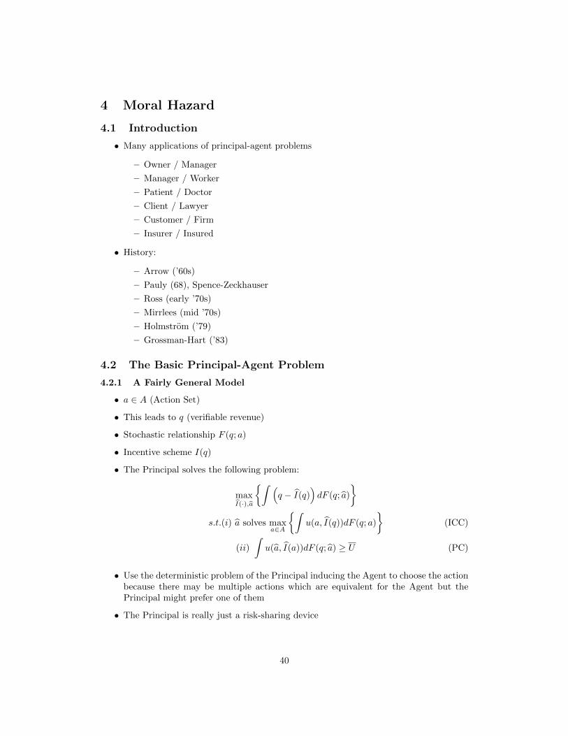
4 Moral Hazard
4.1 Introduction
• Many applications of principal-agent problems
– Owner / Manager
– Manager / Worker
– Patient / Doctor
– Client / Lawyer
– Customer / Firm
– Insurer / Insured
• History:
– Arrow (’60s)
– Pauly (68), Spence-Zeckhauser
– Ross (early ’70s)
– Mirrlees (mid ’70s)
– Holmstrom (’79)
– Grossman-Hart (’83)
4.2 The Basic Principal-Agent Problem
4.2.1 A Fairly General Model
• a ∈ A (Action Set)
• This leads to q (verifiable revenue)
• Stochastic relationship F (q; a)
• Incentive scheme I(q)
• The Principal solves the following problem:
maxI(·),a
{∫ (q − I(q)
)dF (q; a)
}s.t.(i) a solves max
a∈A
{∫u(a, I(q))dF (q; a)
}(ICC)
(ii)
∫u(a, I(a))dF (q; a) ≥ U (PC)
• Use the deterministic problem of the Principal inducing the Agent to choose the actionbecause there may be multiple actions which are equivalent for the Agent but thePrincipal might prefer one of them
• The Principal is really just a risk-sharing device
40

4.2.2 The First-Order Approach
• Suppose A ⊆ R
• The problem is now
maxa,I(·)
{∫ q
q
(q − I(q))f(q|a)dq
}subject to
a ∈ arg maxa∈A
{∫ q
q
u(I(q))f(q |a|)dq −G(a)
}(ICC)∫ q
q
u(I(q))f(q |a|)dq −G(a) > U (PC)
• IC looks like a tricky object
• Maybe we can just use the FOC of the agent’s problem
• That’s what Spence-Zeckhauser, Ross, Harris-Raviv did
• FOC is ∫ q
q
u(I(q))fa(q|a)dq = G′(a)
• SOC is ∫ q
q
u(I(q))faa(q|a)dq = G′′(a)
• If we use the first-order condition approach:
∂
∂I= 0⇒ −f(q; a) + µu′(I(q))fa(q|a) + λu′(I(q))f(q|a)) = 0
⇒ 1
u′(I(q))= λ+ µ
fa(q; a)
f(q; a)
• fa/f is the likelihood ratio
• I ↑ q ⇔ faf ↑ q
• But the FOC approach is not always valid – you are throwing away all the globalconstraints
• The I (q) in the agent’s problem is endogenous!
• MLRP ⇒ “the higher the income the more likely it was generated by high effort”
Condition 1 (Monotonic Likelihood Ratio Property (“MLRP”)). (Strict) MLRP holds if,given a, a′ ∈ A, a′ � a⇒ πi(a
′)/πi(a) is decreasing in i.
Remark 13. It is well known that MLRP is a stronger condition than FOSD (in thatMLRP ⇒ FOSD, but FOSD 6⇒ MLRP).
41

Condition 2 (Covexity of the Distribution Function Condition). Faa ≥ 0.
Remark 14. This is an awkward and somewhat unnatural condition–and it has little or noeconomic interpretation. The CDFC holds for no known family of distributions
• MLRP and CDFC ensure that it will be valid (see Mirrlees 1975, Grossman and Hart1983, Rogerson 1985)
• FOC approach valid when FOC≡ICC
• In general they will be equivalent when the Agent has a convex problem
• To see why (roughly) they do the trick suppose that I (q) is almost everywhere differ-entiable (although since it’s endogenous there’s no good reason to believe that)
– The agent maximizes ∫ q
q
u(I(q))f(q|a)dq −G(a)
– Integrate by parts to obtain
u(I(q))−∫ q
q
u′ (I (q)) I ′ (q)F (q|a)dq −G(a)
– Now differentiate twice w.r.t. a to obtain
−∫ q
q
u′ (I (q)) I ′ (q)Faa(q|a)dq −G′′(a) (*)
– MLRP implies that I ′ (q) ≥ 0
– CDFC says that Faa(q|a) ≥ 0
– G′′ (a) is convex by assumption
– So (*) is negative
• Jewitt’s (Ecta, 1988) assumptions also ensure this by restricting the Agent’s utilityfunction such that this is the case
• Grossman and Hart (Ecta, 1983), proposed the LDFC, (initially referred to as theSpanning Condition).
• Mirrlees and Grossman-Hart conditions focus on the Agent controlling a family ofdistributions and utilize the fact that the ICC is equivalent to the FOC when thefamily of distributions controlled by the Agent is one-dimensional in the distributionspace (which the LDFC ensures), or where the solution is equivalent to a problem witha one-dimensional family (which the CDFC plus MLRP ensure)
Remark 15. Single-dimensionality in the distribution space is not equivalent to the Agenthaving a single control variable – because it gets convexified
• It is easy to see why the LDFC works because it ensures that the integral in the ICconstraint is linear in e.
42

4.2.3 Beyond the First-Order Approach I: Grossman-Hart
Grossman-Hart with 2 Actions
• Grossman-Hart (Ecta, 1983)
• Main idea of GH approach: split the problem into two step
– Step 1: figure out the lowest cost way to implement a given action
– Step 2: pick the action which maximizes the difference between the benefits andcosts
• A = {aL, aH} where aL < aH (in general we use the FB cost to order actions–thisinduces a complete order over A if A is compact)
• Assume q = q1 < ... < qn
• Note: a finite number of states
• Payment from principal to agent is Ii in state i
• aH → (π1(aH), ..., πn(aH))
• aL → (π1(aL), ..., πn(aL))
• Agent has a v-NM utility function U(a, I) = V (I)−G(a)
• G(aH) > G(aL)
• Reservation utility of U
• Assume V defined on (I,∞)
• V ′ > 0, V ′′ < 0, limI→I
V (I) = −∞ (avoid corner solutions, like ln(I) instead of I1/2)
• Of course, a legitimate v-NM utility function has to be bounded above and below (aresult due to Arrow), but...
First Best (a verifiable):
• Define h ≡ V −1
• V (h(V )) = V
• Pick a
• Let CFB(a) = h(U +G(a))
• since V (I)−G(a) = U, V (I) = G(a) + U, I = h(U +G(a))
• Can write the problem as
maxa∈A{ni=1πi(a)qi − CFB(a)}
43

Second Best:
• a = aL then pay you CFB(aL) regardless of the outcome
• a = aH
minI,...,In
{n∑i=1
πi(aH)Ii
}
s.t.(i)
n∑i=1
πi(aH)V (Ii)−G(aH) ≥n∑i=1
πi(aL)V (Ii)−G(aL) (ICC)
(ii)
n∑i=1
πi(aH)V (Ii)−G(aH) ≥ U (PC)
• We use the V s as control variables (which is OK since V is strictly increasing in I)
• vi = V (Ii)
minv1,...,vn
{n∑i=1
πi(aH)h(vi)
}(*)
s.t.(i)
n∑i=1
πi(aH)vi −G(aH) ≥n∑i=1
πi(aL)vi −G(aL) (ICC)
(ii)
n∑i=1
πi(aH)vi −G(aH) ≥ U (PC)
• Now this is just a convex programming problem
• Note, however, that the constraint set is unbounded – need to be careful about theexistence of a solution
Claim 1. Assume πi(aH) > 0,∀i. Then ∃ a unique solution to (*)
Proof. (sketch): The only way there could not be a solution would be if there was anunbounded sequence (v′1, ..., v
′n)⇒ Is are unbounded above⇒ V arI →∞, where Ii = h(vi).
V˜
unbounded ⇒ I˜
unbounded above (if not Is→ I and vs→ −∞ ⇒PC violated. With
V (·) strictly concave E[I˜] → ∞ as I
˜→ ∞ if I 6= −∞. If I = −∞ the PC will be violated
because of risk-aversion.
• Solution must be unique because of strict convexity with linear constraints
• πis are all positive
• Let the minimized value be C(aH)
• Compare∑ni=1 πi(aH)qi − C(aH) to
∑ni=1 πi(aL)qi − CFB(aL)
• This determines whether you want aH or aL in the second-best
44

Claim 2. C(aH) > CFB(aH) if G(aH) > G(aL). The second-best is strictly worse than thefirst-best if you want them to take the harder action.
Proof. (sketch): Otherwise the ICC would be violated because all of the πis are positiveand so all the vs would have to be equal - which implies perfect insurance.
Claim 3. The PC is binding
Proof. (sketch): If∑ni=1 πi(aH)vi−G(aH) > U then we can reduce all the vis by ε and the
Principal is better off without disrupting the ICC.
• FB=SB if:
1. Shirking is optimal
2. V is linear and the agent is wealthy (risk neutrality) – make the Agent the residualclaimant (but need to avoid the wealth constraint)
3. ∃i sth πi(aH) = 0, πi(aL) > 0 (MOVING SUPPORT). If the Agent works hard theyare perfectly insured, if not they get killed.
• Now form the Lagrangian:
=
n∑i=1
πi(aH)h(vi)
−µ
(n∑i=1
πi(aH)vi −G(aH)−n∑i=1
πi(aL)vi +G(aL)
)
−λ
(n∑i=1
πi(aH)vi −G(aH)
)
• The FOCs are:∂
∂vi= 0,∀i
πi(aH)h′(vi)− µπi(aH) + µπi(aL)− λπi(aH) = 0
1
V (Ii)= h′(vi) = λ+ µ− µ πi(aL)
πi(aH)∀i = 1, ..., n
• Note that µ > 0 since if it was not then h′(vi) = λ which would imply that the vis areall the same, thus violating the ICC
• Implication: Payments to the Agent depend on the likelihood ratio πi(aL)πi(aH)
Theorem 9. In the Two Action Case, Necessary and Sufficient conditions for a monotonicincentive scheme is the MLRP
• This is because the FOC approach is valid the in the 2 action case even w/out theCDFC
45

• This behaves like a statistical inference problem even though it is not one (because theactions are endogenous)
• Linearity would be a very fortuitous outcome
• Note: in equilm the Principal knows exactly how much effort is exerted and thedeviations of performance from expectation are stochastic – but this is optimal exante
4.2.4 Beyond the First-Order Approach II: Holden (2005)
Introduction
• Grossman-Hart approach works well for 2 actions, but for n actions it has a difficulty
– First step can be transformed into a convex programming problem
– But step 2 is generally just a non-convex problem
– The C (a) function is a tricky customer
• Standard view: little can be said in the general moral hazard problem (Mirrlees, 1975;Grossman-Hart 1983)
• First-order approach very restrictive – MLRP + CDFC hold for no common family ofdistributions
• Two outcomes or linear contracts very restrictive
• Just saw that the optimal contract is highly non-linear (Mirrlees’s “Unpleasant The-orem”)
• Grossman-Hart (1983): decompose the problem into two steps
– Step One: Find lowest cost way to implement a given action
– Step Two: Choose the action which maximizes difference b/w benefits and costs
– Show how to do step one
– Step two generally a non-convex problem
• Holden (2005) – can do comparative statics on step two
– Multiple optima can be handled with lattice theory
Introductory Lattice Theory
• Implicit function theorem usually used to do comparative statics
• Can’t handle non-convexities or multiple optima
• Topkis (1978) – maximizing a supermodular function on a lattice
– Nice comparative static properties
– Primitives of theory are a set and a partial order to compare elements
46

– Nice and simple in Rn
Definition 16. A set X is a “Product Set” if ∃ sets X1, ..., Xn such that X = X1× ...×Xn.X is a Product Set in Rn if Xi ⊆ R, i = 1, ..., n.
• eg. unit square is a product set in R2
• Doesn’t need to be an interval
Definition 17. A function f : X → R has Increasing Differences in (xn;xm) , n 6= m iff∀x′n ∈ Xn and x′′n ∈ Xn with x′n > x′′n, and ∀xj , j 6= n,m we have
f(x1, ..., x′n, ..., xN )− f (x1, ..., x
′′n, ..., xN ) is nondecreasing in xm
• If f is differentiable in xn then f has increasing differences in (xn;xm) iff
∂
∂xnf (·) is nondecreasing in xm
• If f is C2 then we need:∂2
∂xn∂xmf ≥ 0
• Intuition: raising the level of xm weakly increases the return to raising xn.
Definition 18. If f has increasing differences in (xn;xm)∀n 6= m then f is Supermodular
• When multiple optima exist want to be able to talk about sets being higher than eachother
Definition 19. A set S ⊆ R is said to be as “High” as another set T ⊆ R (S ≥S T ), ifand only if (i) each x ∈ S\T is greater than each y ∈ T, and (ii) each x′ ∈ T\S is less thaneach y′ ∈ S.
itbpFU5.2849in2.1672in0inTheStrongSetOrderF igure
The Approach
Statement of the Problem
• Risk-neutral principal and a risk-averse agent
• Let φ be a parameter of interest which affects gross profits
• A finite number of possible gross profit levels for the firm. Denote these q1(φ) < ... <qn(φ). These are profits before any payments to the agent.
• The set of actions available to the agent is A which is assumed to be a product set inRn, non-empty, and compact.
• Let S be the standard probability simplex, i.e. S = {y ∈ Rn|y ≥ 0,∑ni=1 yi = 1}
• Assume that there is a twice continuously differentiable function π : A→ S
47
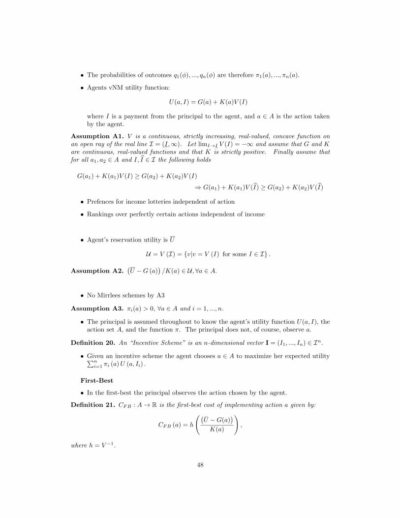
• The probabilities of outcomes q1(φ), ..., qn(φ) are therefore π1(a), ..., πn(a).
• Agents vNM utility function:
U(a, I) = G(a) +K(a)V (I)
where I is a payment from the principal to the agent, and a ∈ A is the action takenby the agent.
Assumption A1. V is a continuous, strictly increasing, real-valued, concave function onan open ray of the real line I = (I,∞). Let limI→I V (I) = −∞ and assume that G and Kare continuous, real-valued functions and that K is strictly positive. Finally assume thatfor all a1, a2 ∈ A and I, I ∈ I the following holds
G(a1) +K(a1)V (I) ≥ G(a2) +K(a2)V (I)
⇒ G(a1) +K(a1)V (I) ≥ G(a2) +K(a2)V (I)
• Prefences for income lotteries independent of action
• Rankings over perfectly certain actions independent of income
• Agent’s reservation utility is U
U = V (I) = {v|v = V (I) for some I ∈ I} .
Assumption A2.(U −G (a)
)/K(a) ∈ U ,∀a ∈ A.
• No Mirrlees schemes by A3
Assumption A3. πi(a) > 0, ∀a ∈ A and i = 1, ..., n.
• The principal is assumed throughout to know the agent’s utility function U(a, I), theaction set A, and the function π. The principal does not, of course, observe a.
Definition 20. An “Incentive Scheme” is an n-dimensional vector I = (I1, ..., In) ∈ In.
• Given an incentive scheme the agent chooses a ∈ A to maximize her expected utility∑ni=1 πi (a)U (a, Ii) .
First-Best
• In the first-best the principal observes the action chosen by the agent.
Definition 21. CFB : A→ R is the first-best cost of implementing action a given by:
CFB (a) = h
((U −G(a)
)K(a)
),
where h = V −1.
48

• The contract involved in achieving the first-best is the following. The principal paysthe agent CFB (a) if she chooses a and some I otherwise, where I is “close” to I.
Definition 22. The First-Best action is that which solves:
maxa∈A
{n∑i=1
πi (a) qi (φ)− CFB (a)
}.
Note that CFB induces a complete ordering on A, which is independent of U .
Notation 4. a � a′ ⇔ CFB (a) ≥ CFB (a′) .
Second-Best Step One: Lowest Cost Implementation In the second-best theproblem which the principal faces is to choose an action and a payment schedule to maximizeexpected output net of payments, subject to that action being optimal for the agent andsubject to the agent receiving her reservation utility in expectation.
maxa,(I1,...,In)
{n∑i=1
(πi(a) (qi − Ii))
}(7)
subject to
a∗ ∈ arg maxa
{n∑i=1
πi(a)U(a, Ii)
}n∑i=1
πi(a∗)U(a∗, Ii) ≥ U
minI1,...,In;Ii∈I,∀i
{n∑i=1
πi(a∗)Ii
}(8)
subject to
a∗ ∈ arg maxa
{n∑i=1
πi(a)U(a, Ii)
}n∑i=1
πi(a∗)U(a∗, Ii) ≥ U
Now define υ1 = V (I1), ..., υn = V (In) and h ≡ V −1. These will be used as the control
49

variables. The problem can now be stated as:
minυ1,...,υn;vi∈U,∀i
{n∑i=1
πi(a∗)h(υi)
}(9)
subject to
G(a∗) +K(a∗)
(n∑i=1
πi(a∗)υi
)≥ G(a) +K(a)
(n∑i=1
πi(a)υi
),∀a ∈ A
G(a∗) +K(a∗)
(n∑i=1
πi(a∗)υi
)≥ U
• The constraints in (9) are linear in the υjs and, since V is concave, h is convex.Consequently the problem in (9) is simply to minimize a convex function subject to aset of linear constraints. Since A is a compact subset of a finite dimensional Euclideanspace the Karush-Kuhn-Tucker Theorem provides necessary and sufficient conditionsfor a minimum. For A infinite Weierstrass’s Theorem establishes the existence of aminimum.
Definition 23. A vector (υ1, ..., υn) which satisfies the constraints in (9) or (I1, ..., In)which satisfies the constraints in (8) is said to “Implement” action a∗.
Definition 24. Let:
C(a∗) = inf
{n∑i=1
πi(a∗)h(υi)|υ = (υ1, ..., υn) implements a∗
}
which implements a∗ if the constraint set in (9) is non-empty. If the constraint set is emptythen let C(a∗) =∞.
Second-Best Step Two: Monotone Comparative Statics on the Optimal Ac-tion
• The second-step of the Grossman-Hart approach is to choose which action should beimplemented
• i.e choose the action which maximizes the expected benefits minus the costs of imple-mentation:
maxa∈A{B(a, φ)− C(a)} (10)
where B(a, φ) =∑ni=1 πi(a)qi(φ).
Definition 25. Generally a non-convex problem, for C (a) will not generally be a convexfunction.
• Denote a∗∗(φ;C) = arg maxa∈A {B(a, φ)− C(a)} as the solution to the problem.
• What does it mean for a set of optima to increase? SSO.
50

Proposition 4. a∗∗(φ;C) is nondecreasing in φ for all functions C iff B has increasingdifferences.
Proof. Follows directly from Athey-Milgrom-Roberts Theorem 2.3.
• This result deals with the possibility that all of the local optima are nondecreasing inφ but that the global optimum is actually decreasing in φ for some values1.
ftbphFU2.3393in2.2969in0ptAn increase in φ leads to a harder actionFigureftbphFU2.4647in2.4491in0ptAn increase in φ leads to an easier actionFigure
Assumption A4. A ⊆ R
Assumption A5. B is twice continuously differentiable in both its arguments.
Lemma 1. Assume A4-A5. Then B has increasing differences iff:
n∑i=1
q′i(φ)π′i(a) ≥ 0,∀a, φ.
Proof. Athey-Milgrom-Roberts Theorem 2.2 demonstrates that a function f(x, θ) whichis twice continuously differentiable has increasing differences if and only if for all x, θ,∂2
∂x∂θf(x, θ) ≥ 0. Now note that ∂2
∂a∂φB is∑ni=1 q
′i(φ)π′i(a).
• We will sometimes be interested in a strict comparative static - a∗∗(φ;C) strictlyincreasing in φ (as opposed to merely nondecreasing).
• A function can have strictly increasing differences2 but have the maximum not increasein the relevant parameter
Proposition 5. Assume A4-A5, that C(a) is continuously differentiable, and that a∗∗(φ;C) ∈int (A) for all φ. Then a∗∗(φ;C) is strictly nondecreasing in φ for all functions C iff∂2
∂a∂φB > 0.
Proof. See AMR Theorem 2.6
Remark 16. Edlin and Shannon (1998) show that A4 is not required for this result, andthat A5 can be weakened to only require B to be continuously differentiable in a.
By construction, an increase in effort affects the probabilities of different states occurring.
Assumption A6. π : A → S satisfies First Order Stochastic Dominance (“FOSD”) ifa1 > a2 ∈ A⇒
∑i πi(a1) <
∑i πi(a2),∀i < n.
1See, for instance, AMR figure 2.1 and the accompanying discussion.2A function f : R2 → R has “Strictly Increasing Differences” if for all x′′ > x′, f(x′′, θ) − f(x′, θ) is
strictly increasing in θ.
51

Two Outcomes
• Denote the two possible outcomes as H and L. Lemma 1 implies that for a∗∗ to benondecreasing in φ requires:
q′L(φ)π′L(a) + q′H(φ)π′H(a) ≥ 0 (11)
• By definition πL(a)+πH(a) = 1. Differentiating this identity yields π′L(a)+π′H(a) = 0.Therefore π′H(a) = −π′L(a) and one can write (11) as:
π′L(a) [q′L(φ)− q′H(φ)] ≥ 0
• Since a harder action makes the low profit state less likely by FOSD, it must be thatπ′L(a) ≤ 0. Therefore we require q′L(φ)−q′H(φ) ≤ 0, which amounts to q′H(φ) ≥ q′L(φ).
• If φ reduces profit less, or increases it more, in the high profit state (i.e. q′H(φ) >q′L(φ)), then a higher value of φ leads to a harder action.
• If a higher value of φ makes the high profit state relatively more attractive to theprincipal, then she induces the agent to put more probability weight on that state by“twisting” the incentive scheme in that direction.
4.2.5 Value of Information
• Say there is a signal which is realized after effort is chosen by the Agent but beforethe realization of the outcome such that :
πij(a) = π(i, j | a)
• ie. probability of outcome i, signal j conditional on action a
• Signal does not enter directly into objective functions – only though the probabilities
• Now, letting ψ(a) be the cost of effort, the Principal solves:
max
∑i,j
πij(a)V (i− wij)
s.t.(i)
∑i,j
πij(a)u(wij)− ψ(a) ≥ U (PC)
(ii)a ∈ arg max
∑i,j
πij(a)u(wij)− ψ(a)
(ICC)
• Put the Lagrange multiplier λ on the PC
• The ICC FOC is∑π′ij(a)u(wij) = 1
52

• Forming the Lagrangian and finding ∂∂wi
= 0,∀i,∀j yields:
V ′(i− wij)u′(wij)
= λ+ µπ′ij(a)
πij(a)(12)
• When is the optimal wij independent of j ?
• Same as before ifπ′ij(a)
πij(a)=π′i(a)
πi(a)
• In the continuum case this is just:
ga (q, s|a)
g (q, s|a)=fa (q, s|a)
f (q, s|a)
• Integrating this object with respect to a means that it is equivalent to the existenceof two function m (q|a) and n (q|s) such that:
g (q, s|a) = m (q|a)n (q|s) .
• That is, that q is a sufficient statistic for the pair (q, s) with respect to a
• This representation is known as the Halmos-Savage factorization criterion (or theorem)– see DeGroot (1971) for further details
• So, the optimal incentive scheme is conditioned on s if and only if s is informativeabout a, given that q is already available
4.2.6 Random Schemes
• Can one do better with random schemes? Do you want to add noise ?
• Suppose the Principal decided to “flip a coin”, j ∈ {1, ...,m} → pr(j) = q(j)
• πij(a) = qjπi(a)
• Suppose wij was the optimal scheme and let wi be the certainty equivalent:
u(wi) =∑j
qju(wij) ,∀i
• But we haven’t changed the ICC or PC
• However, the Principal has cost wi and wi <∑j qjwij due to the concavity of u(·).
So the Principal is better off. Contradiction
• Therefore random schemes cannot be better
• They put more risk onto the risk-averse Agent and that requires the Agent to becompensated for bearing that risk
53

• Can also use the sufficient statistic result - the random scheme adds no informationabout the likelihood ratio (and generalizes to the case where the Principal is risk-averse)
4.2.7 Linear Contracts
• Very little that you can say in a general moral hazard model (Grossman and Hart 83)
• Say w = t+ vq
• Assume normally distributed performance and CARA (exponential) utility
• Let q = a+ ε with ε ∼ N(0, σ2)
• Assume the Principal is risk-neutral
• The Agent is risk-averse with:
U(w, a) = −e−r(w−ψ(a))
• Let ψ(a) = ca2
2
• Note that r is the coefficient of absolute risk-aversion −u′′/u′
• The Principal solves:
maxa,t,v
E[q − w]
s.t.(i)E[−e−r(w−ψ(a))] ≥ −e−rw (PC)
(ii)a ∈ arg maxa
E[−e−r(w−ψ(a))] (ICC)
• Let x ∼ N(0, σ2x)
• E[eγx] = eγ2σ2x/2 (this is essentially the calculation done to yield the moment gener-
ating function of the normal distribution – see Varian for a more detailed derivation)
E[−e−r(w−ψ(a))]
= −E[−e−r(t+va+vε−ψ(a))]
= −e−r(t+va−ψ(a))E[e−rvε]
= e−rw(a)
• w(a) = t+ va− r2v
2σ2 − 12ca
2
• Now maxa{w(a)}
• FOC is v − ca = 0⇒ a = v/c
54

• Replace a with v/c in the Principal’s Problem and they solve:
maxv,t
{v
c− (t+
v2
c)
}(13)
s.t.w(a) = w(v
c) = wPC (14)
• The PC is, written more fully:
t+v2
c− r
2v2σ2 − v2
2c
• ie.
t+v2
2c− r
2v2σ2 = w
• Substituting for t:
maxv
{v
c− v2
c+v2
2c− r
2v2σ2 − w
}• The FOC is:
1
c− v
c− rvσ2 = 0
• Hence:
v =1
1 + rcσ2
• Which is a nice, simple, closed form solution
• But the linearity restriction is not at all innocuous
• In fact, linear contracts are not optimal in this setting!
• Without the restriction one may approximate the first-best
Example 1: Moving Support
• q = a+ ε and ε is uniformly distributed on [−k, k] with k > 0
• So the Agent’s action moves the support of q
Claim 4. The first-best can be implemented by a non-linear contract
Proof. Let a∗ be the first-best level of effort. q will take values in [a∗− k, a∗+ k]. Scheme:pay w∗ whenever q ∈ [a∗−k, a∗+k] and pay −∞ otherwise. Just a Mirrlees Scheme (whichis certainly not linear)
• With bounded support the Principal can rule out certain outcomes provided the Agentchooses the FB action.
Example 2:
55

• q = a+ ε and ε ∼ N [0, σ2]
⇒ f(q, a) =1
(2πσ)1/2
e−(q−a)2/2σ2
• Calculate the likelihood ratio:
fa(q, a) = − 1
(2πσ)1/2
e−(q−a)2/2σ2
× −(q − a)
σ2
• faf = q−a
σ2
• as q →∞+, faf →∞
• So the likelihood ratio can take on values on (−∞,∞)
• For extreme values (ie. in the tails of the distn) the Principal gets almost perfectinformation
Claim 5. FB a∗ can be arbitrarily approximated
Proof. Suppose the Principal chooses an incentive scheme as follows: if q < q → low transferk, if q ≥ q → transfer w∗. Suppose the Agent has a utility function u(y), u′(y) > 0, u′′(y) < 0and cost of effort ψ(a). To implement a∗ under the above scheme we need that:
IC :
∫ q
−∞u(k)fa(q, a∗)dq +
∫ ∞q
u(w∗(q))fa(q, a∗)dq = ψ′(a∗)
But this violates the PC by:
l =
∫ q
−∞[u(w∗(q))− u(k)] f(q∗)dq
Claim 6. One can choose q and k to make l arbitrarily small.
Proof. Given −M,∃q such that:
fa(q, a)
f(q, a)≤ −M for q ≤ q
⇒ faf
(−1M
)≥ 1⇔ f ≤ fa(−1
M )
⇒ l ≤∫ q
−∞[u(w∗(q))− u(k)] fa(q∗, a)
(−1
M
)dq
=−1
M(·)
Therefore one can make l arbitrarily small by making M arbitrarily large
56

• The expected punishment is bounded away from ∞
• Mirrlees’s (1974) idea again – this time without the moving support
• Although the size of the punishment grows, its frequency falls at a faster rate
4.3 Multi-Agent Moral Hazard
4.3.1 Relative Performance Evaluation
• Holmstrom (Bell, 1982)
• Assume for simplicity 2 symmetric agents
• q1 = a1 + ε1 + βε2
• q2 = a2 + ε2 + βε1
• ε1 and ε2 are iid N(0, σ2
)• Principal is risk-neutral
• Agents are risk-averse
• Agents have utility functions of the form:
U(a,w) = −e−r(w−ψ(a))
• where ψ(a) = 12ca
2
• Assume linear contracts so that:
w1 = t1 + v1q1 + u1q2
w2 = t2 + v2q2 + u2q1
• u1 = u2 = 0 is the case of no relative performance evaluation
• The Principal solves:
maxa1,t1,v1,u1
E[q1 − w1]
s.t.(i) E[−e−r(w1− 12 ca
2)] ≥ −e−rw (PC)
(ii) a1 ∈ arg maxa
E[−e−r(w1− 12 ca
2)] (ICC)
• where w is the reservation wage
57

• The Agent’s payoff is w1 − 12ca
21
= t1 + v1q1 + u1q2 −1
2ca2
1
= t1 + v1(a1 + ε1 + βε2) + u1(a2 + ε2 + βε1)− 1
2ca2
1
• The certainty equivalent (“CE”) of this is:
CE = t1 + v1a1 + u1a2 −r
2σ2((v1 + βu1)2 + (u1 + βv1)2)− 1
2ca2
1
since
risk = var (v1(a1 + ε1 + βε2) + u1(a2 + ε2 + βε1))
= var (v1(ε1 + βε2) + u1(ε2 + βε1))
= σ2[(v1 + βu1)
2+ (u1 + βv1)
2]
• The FOC is:
∂CE
∂a1⇒ v1 = ca1
a1 =v1
c
• The Principal solves:
maxt1,v1,a1
{v1
c− (t1 + v1
v1
c+ u1a2)
}s.t.CE = w
• Which is equivalent to:
maxv1,u1
{v1c −
v21c − w +
v21c − u1a2 + u1a2
− r2σ2((v1 + βu1)2 + (u1 + βv1)2)− 1
2cv21c2
}
• Simplification yields:
maxv1,u1
{v1
c− v2
1
2c− r
2σ2((v1 + βu1)2 + (u1 + βv1)2)
}• Trick: given v1, u1 is determined to minimize risk; then v1 is set to trade-off risk
sharing and incentives
• Fix v1 and solve:minu1
{(v1 + βu1)2 + (u1 + βv1)2
}⇒ 2(v1 + βu1) + 2(u1 + βv1) = 0
58

u1 =−2β
1 + β2v1
• u1 = 0 if β = 0 (ie. the environments are completely independent)
• Filter out the common shock
• This implies that:
v1 =1
1 + rσ2c (1−β2)2
1+β2
• It doesn’t matter whether β ≶ 0
• You can make incentives more high powered because there is a way to insure the Agent
• Noise is netted out
4.3.2 Moral Hazard in Teams
• Holmstrom (Bell, 1982)
• n agents 1, ..., n who choose actions a1, ..., an
• This produces revenue q(a1, ..., an) with q(·) concave
• Agent’s utility function is Ii − ψi(ai) with ψi(·) convex
• In the first-best:
max
{q(a1, ..., an)−
n∑i=1
ψi(ai)
}
• The FOC is:∂q
∂ai= ψ′i(ai) ,∀i
• In the second-best assume that ai is observable only to agent i but that q is observableto everyone
• A partnership consists of sharing rules si(ai), i = 1, ..., n such that∑i
si(q) ≡ q (15)
• Might suppose that si(q) ≥ 0,∀i
• In a Nash Equilibrium each agent solves:
maxai{si(q (ai, a−i))− ψi(ai)}
• The FOC is:
s′i(q)∂q (ai, a−i)
∂ai= ψ′i(ai)
59

• Need s′i(q) = 1,∀i to get the FB
• But we know from (15) that∑i s′i(q) ≡ 1
• Can’t get the FB
• Nothing to do with risk-aversion – there is no uncertainty here
• Say we introduce an (n+ 1)th party such that:
si(q) ≡ q (a∗)− Fi, ∀i = 1, ..., n
sn+1(q) =∑i
Fi − nq (a∗)
• This will be profitable for the (n+ 1)th party if we pick Fi such that∑ni=1 Fi+q (a∗) ≥
nq (a∗)
• And also profitable for the agents if Fi ≤ q (a∗)− ψi (a∗i )
• These can both be satisfied because at the FB q (a∗)−∑ni=1 ψi (a∗i ) > 0
• We have made everyone the residual claimant
• However, the (n+ 1)th party wants it to fail. They might burn the factory down, ...Call them the Budget Breaker (“BB”)
• They might also collude with one of the Agents
• A side contract between BB and i – this merges BB and i into one person and we areback into the n agent case
• n people could collude to “borrow” q and game the BB
• This mechanism (making everyone the residual claimant) is similar to Groves-Clarkewe we saw earlier
4.3.3 Random Schemes
• Legros & Matthews (Restud, 1993)
• Can get the FB by using a random scheme
• Say n = 2, Ai ∈ {0, 2} , q(a) = a1 + a2, ψi =a2i2
• FB:
maxa1,a2
{a1 + a2 −
1
2a2
1 −1
2a2
2
}• ⇒ a∗1 = a∗2 = 1
60

• SB: Agent 1 a∗1 = 1, Agent 2 a∗2 = 1 with Pr (1− 2δ) , 2 wth Pr (δ) , 0 wtih Pr (δ)
s2(q) =(q − 1)2
2
s1(q) = q − (q − 1)2
2
• Agent 2 indifferent about a2 given a∗1 = 1
• Her payoff is:(1 + a2 − 1)2
2− 1
2a2
2 = 0
• So Agent 2 is perfectly prepared to play the mixed strategy
• Make 1 pay 2 a large fine if q < 1 or q > 3
• Wealth constraint is a very serious problem
• Also give 2 a big incentive not to play the mixed strategy – and as always, it is veryhard to make sure that mixed strategies are verifiable
• It is in general a big problem – as n goes large effort → 0 since FOC⇒ 1n = ψ′(a)
4.3.4 Tournaments
• Lazear and Rosen (JPE, 1981)
• Let q1 = a1 + ε1, q2 = a2 + ε2
• Assume that ε1, ε2 are iid ∼ N(0, σ2)
• The Principal and Agent are risk-neutral
• The winner of the tournament is the one with the higher q and gets the prize w – andboth get a fixed payment t
• Agent i solves:
maxai{E[wi − ψ(ai)]} = max
ai{t+ pw − ψ(ai)}
= maxai{t+ pr(qi > qj)w − ψ(ai)}
= maxai{t+ pr(ai + εi > aj + εj)w − ψ(ai)}
= maxai{t+ pr(εj − εi < ai − aj)w − ψ(ai)}
= maxai{t+G(ai − aj)w − ψ(ai)}
• where G is the CDF of εj − εi
61

• Note that εj − εi ∼ N(0, 2σ2)
• FOCs:g(ai − aj)w − ψ′(ai) = 0
and:g(aj − ai)w − ψ′(aj) = 0
• The symmetric Nash Equilibrium is ai = aj = a
• Hence g(0)w = ψ′(a)
• FB ⇒ ψ′(aFB) = 1
• Therefore:
w =1
g(0)
• Just need an ordinal measure to get the FB
• Risk-neutrality seems like a huge issue – with both risk-neutral we could just useresidual claimancy anyway
• With risk-aversion and a common shock consider a comparison of the piece-rate andthe tournament
– With a big common shock (ie. (ε1, ε2) ∼ N(0,Σ), where Σ =
(σ2 RR σ2
)the tour-
nament dominates because the piece-rate doesn’t take into account the commonshock
– With a small common shock the tournament imposes lots of risk and is thusdominated by the piece-rate scheme
– See Green & Stokey (1983)
• Green-Stokey setup
– P pays a prize wi to the individual who places ith in the tournament
– π =∑ni=1(qi − wi)
– Assume that individuals are homogeneous in ability
– If individual j exerts effort ej , her output is given by qj = ej+εj+η, where εj andη are random variables with mean zero and distributed according to distributionsF and G respectively
– Assume that F and G are statistically independent
– Refer to η as the “common shock” to output and εj as the “idiosyncratic shock”to output
– Each agent’s tility is given by: u(wi)− c(ej) where u′ ≥ 0, u′′ ≤ 0, c′ ≥ 0, c′′ ≥ 0
– Time 0: the principal commits to a prize schedule {wi}ni=1. Time 1: individualsdecide whether or not to participate. Time 2: if everyone has agreed to partici-pate at time 1, individuals choose how much effort to exert. Time 3: output isrealized and prizes are awarded
62

– Restrict attention to symmetric pure strategy equilibria
– A unique symmetric pure strategy equilibrium will always exist, provided thatthe distribution of idiosyncratic shocks is “sufficiently dispersed”
– In a symmetric equilibrium, every individual will exert effort e∗
– Furthermore, every individual has an equal chance of winning any prize and theexpected utility is
1
n
∑i
u(wi)− c(e∗)
– In order for it to be worthwhile for an individual to participate in the tournament,it is necessary that
1
n
∑i
u(wi)− c(e∗) ≥ U
– An individual who exerts effort e while everyone else exerts effort e∗ receivesexpected utility
U(e, e∗) =∑i
ϕi(e, e∗)u(wi)− c(e)
where ϕi(e, e∗) = Pr(ith place|e, e∗),
– that is, the probability of achieving place i given effort e while all other agentschoose effort e∗
– Each agent chooses e to maximize U(e, e∗)
– The first-order condition for this problem is
c′(e) =∑i
∂
∂eϕi(e, e
∗)u(wi)
– Since we know that the solution to the maximization problem is e = e∗, it followsthat
c′(e∗) =∑i
βiu(wi)
where βi =∂
∂eϕi(e, e
∗)
∣∣∣∣e=e∗
– Note that βi does not depend upon e∗ but simply upon the distribution functionF
– Routine results from the study of order-statistics imply that the formula for βi is
βi =
(n− 1
i− 1
)∫R
F (x)n−i−1(1− F (x))i−2 ((n− i)− (n− 1)F (x)) f(x)2dx
Since∑i ϕi = 1, it follows that
∑i βi = 0
– It is also easily shown that if F is a symmetric distribution (F (−x) = 1−F (x)),that βi = −βn+1−i.
63

– Now that we have elaborated the agent’s problem, we turn to the principal’sproblem. The principal’s object is to maximize
E(π) =∑j
ej −∑i
wi = n
(e∗ − 1
n
∑i
wi
).
– The problem of the principal can therefore be stated as follows
maxwi
(e∗ − 1
n
∑i
wi
)subject to
1
n
∑i
u(wi)− c(e∗) ≥ U (IR)
c′(e∗) =∑i
βiu(wi) (IC)
• Tournaments generally suboptimal because they throw away the cardinal information
• RPE individual contracts do better
• Green-Stokey limit result: as the number of players goes to infinite the tournamentgoes to the optimal RPE individual contract
4.3.5 Supervision & Collusion
• Tirole (JLEO, 1986)
• Consider a Principal who wants a service from an Agent
• Suppose that the supply cost c is 0 or 1 with equal probability
• The value of the service to the Principal is s
• The Agent knows c, the Principal does not
• Assume that the Principal has all the bargaining power
• Assume s > Z so that s− 1 > s/2 and hence makes a take-it-or-leave-it offer of 1
• Suppose that the Principal can hire a supervisor at cost z
• The supervisor, with probability p, gets hard evidence that c = 0 when c = 0
• Assume that the evidence can be destroyed, but that it cannot be falsified / fabricated
Case I: Honest Supervisor
• Optimal contract is: if Supervisor reports c = 0 the Agent gets 0, if not the Agentgets 1
64

• The Principal’s payoff is 12ps+ (1− p
2 )(s− 1)− z
• This is greater than s− 1 if z is small enough
Case II: Corrupt Supervisor
• Collusion technology: The Agent can pay the Supervisor t but the Supervisor onlyreceives kt where k ∈ [0, 1] - but other than this, the side relationship is binding
• Tirole introduces the Collusion Proofness Principle – a bit like the Revelation Principle
• Optimal Contract: if produce hard evidence then the Principal pays w
• w ≥ k to avoid collusion, because there is 1 on the table for the Agent which is worthk to the supervisor. Obviously w = k
• The Principal’s payoff, assuming z = 0, is:
p
2(s− k) + (1− p
2)(s− 1)
• With an honest supervisor the payoff is:
ps
2+ (1− p
2)(s− 1)
• The Principal’s payoff without a supervisor is s− 1
• Since k < 1 you always want a supervisor
Comments:
1. Collusion proof principle is not that robust – for instance, if k is random
2. Collusion v. costly effort – rotation of supervisors might be good (make k go down)
3. In some cases you could make the supervisor the residual claimant (eg. speeding fineand police)
4.3.6 Hierarchies
• Qian (Restud, 1994)
• Consider a hierarchy which consists of T layers with top layer being tier 0 and bottomT
• Define the “span of control” as si+1 which is the number of individuals in tier i + 1who are monitored by an individual in tier i
• Let the number of individuals in a tier be Xi
• Assume that XT = N and that output is given by θNyT where θ is a measure ofprofitability, N is the scale and yT is the effective output per final worker
65

• Assume that there is a ”loss of control” represented by yt = atyt−1 with at ≤ 1
• Assume that the Principal has no incentive problem so that a0 = 1 and that for allother tiers there is a convex effort cost g(a) = a3
• Let w be the wage and p = 1/si be the probability of getting caught when shirking
• The program for the optimal organizational design is:
maxst,at,xt,T
{θNyt −
T∑t=1
g(at)stxt
}s.t.(i) xt = xt−1st
(ii) yt − yt−1at
(iii) x0 = y0 = 1, xT = N
(iv) 0 ≤ at ≤ 1,∀t
Results:
Proposition 6. Assume that T = 1 which means that there is one Principal and N workers
so that y1 = y0a = a, x1 = x0s = N, s1 = N. Then a = min{
1, (θ/3)1/2
N−1/2}.
Proof. Introducing some new notation, the program to be solved is now:
Π1 = maxa∈[0,1]
{θNa− a3N2
}The first-order condition is:
θN = 3a2N2
⇒ a = min{
1, (θ/3)1/2
N−1/2}
Proposition 7. Now assume that T = 2. Then a∗1 = 1 and a∗2 ≤ a∗1.
Proof. Note that T = 2 ⇒ N = x2 = x1s2, x1 = x0s1 = s1, y1 = y0a1 = a1, y2 = y1a2 =a1a2. Now write an unconstrained program with a1, a2, x1 as control variables as follows:
maxa1,a2,x1
{θNa1a2 − a3
1x21 − a3
2N2/x1
}(16)
First fix a1 and a2 and optimize with respect to x1. This yields the first-order condition:
−2x1a31 + a3
2N2/x2
1 = 0
This implies:
x1 =a3
2N2
2a31
=a2
a1
(N2
2
)1/3
66

Now substitute into (16):
maxa1,a2
{θNa1a2 − a1a
22
[(N2
2
)2/3
+
(2
N2
)1/3
N2
]}
Note that: (N2
2
)2/3
+
(2
N2
)1/3
N2 = N4/3(
2−2/3 + 21/3)
and denote(2−2/3 + 21/3
)as z < 2. This directly implies that a∗1 = 1 since if it were less
than 1 then increasing it to 1 and reducing a2 to keep a1a2 constant increases the maximand.Therefore a∗2 ≤ a∗1 = 1.
• This means that effort goes down when one moves down the hierarchy. Intuitively,the higher up the hierarchy, the more yT ’s are being affect by effort which raises themarginal benefit of effort as one moves up the hierarchy.
• Now we can offer a necessary and sufficient condition for profit under T = 2 to begreater than under T = 1.
Π2 = maxa2
{θNa2 − a2
2N4/3z
}
• Solving for a2 from above yields:
a2 = min{
1, (θ/2z)N−1/3}
and then:Π2 > Π1 ⇔ θ1/2N1/6 ≥ 3
• This means that it is optimal to increase the number of layers in the hierarchy if Nbecomes sufficiently large. The intuition for this is as follows. An increase in N meansless supervision for T = 1, and therefore a reduction in effort since compensating thedecrease in supervision by an increase in wages is prohibitively costly. So an increasein N increases the gain of having an intermediate layer so as to save on wages at thebottom of the hierarchy.
Proposition 8. The amount of wage inequality w1/w2 is increasing in N.
Proof. With T = 1 we have:
w = g(a)s
= g(a)N
=
(θ
3
)3/2
N−1/2
67

With T = 2:
w1 = g(a1)s1
= a31
a2
a1
(N2
2
)1/3
= a2
(N2
2
)1/3
=
(θ
2z
)N1/321/3
and:
w2 = g(a2)s2
= g(a2)N
x1
=
(θ
2z
)2
N−1/321/3
It is therefore clear that ∂w1
∂N > 0 and ∂w2
∂N < 0. This directly implies that ∂ (w1/w2) /∂N >0. Therefore wage inequality is increasing in N.
4.4 Moral Hazard with Multiple Tasks
4.4.1 Holmstrom-Milgrom
• Holmstrom-Milgrom (JLEO, 1991)
• Different tasks with different degrees of measurability
• Suppose the Agent can sell the Principal’s product or someone else’s product
• 2 tasks i = 1, 2
• Let qi = ai + εi
• (ε1, ε2) ∼ N(0,Σ) where
Σ =
(σ2
1 RR σ2
2
)• Let the Agent’s utility be given by:
−e−r(w−ψ(a1,a2))
• where ψ(a1, a2) = 12 (c1a
21 + c2a
22) + δa1a2
• if δ > 0 then the two tasks are technological substitutes, if δ < 0 they are complements
• Assume a linear incentive scheme:
w = t+ v1q1 + v2q2
68

w(a1, a2) = E[w(a1, a2)]− r
2var (w(a1, a2))− ψ(a1, a2)
= E[t+ v1 (a1 + ε1) + v2 (a2 + ε2)]
−r2var(t+ v1 (a1 + ε1) + v2 (a2 + ε2))
−1
2((c1a
21 + c2a
22) + δa1a2)
• E[t+ v1 (a1 + ε1) + v2 (a2 + ε2)] = t+ v1q1 + v2q2
• V ar(·) = v21σ
21 + v2
2σ22 + 2Rv1v2
• The Agent solves:maxa1,a2
{w(a1, a2)}
• Let R = 0
• The FOCs are now:v1 = c1a1 + δa2
v2 = c2a2 + δa1
• Using the FOC approach the Principal solves:
maxv1,v2,a1,a2
{E[q − w] = a1 + a2 − t− v1a1 − v2a2}
s.t.(i) w(a1, a2) = t+ v1a1 + v2a2
−r2
(v2
1σ21 + v2
2σ22 + 2Rv1v2
)≥W
(ii) v1 = c1a1 + δa2
(iii) v2 = c2a2 + δa1
• (i) must bind so we have:
maxv1,v2,a1,a2
{a1 + a2 − r
2
(v2
1σ21 + v2
2σ22 + 2Rv1v2
)− 1
2
(c1a
21 + c2a
22
)− δa1a2
}s.t. v1 = c1a1 + δa2
v2 = c2a2 + δa1
• FOC1:1− rσ2
1v1c1 − rσ22v2δ − v1 = 0
• ⇒v1 =
1− rσ22v2δ
1 + rσ21v1c1
69

v2 =1− rσ2
1v1δ
1 + rσ22v2c2
• Solving simultaneously yields:
v1 =1 + rσ2
2(c2 − δ)1 + rσ2
1c1 + rσ22c2 + r2σ2
1σ22(c1c2 − δ2)
• and symmetrically for v2
Results:
1. Go from δ = 1 to δ = −1 (ie. substitutes to compliments) and v1, v2 increase
2. When δ = 0 :
v1 =1
1 + rσ21c1
which is simply the one-task case.
3. As σ22 →∞ (task 2 is really hard to measure) then:
v2 → 0
v1 →r(c2 − δ)
rc2 + r2σ21(c1c2 − δ2)
Put all the incentive on task 1.
4.5 Dynamic Moral Hazard
4.5.1 Stationarity and Linearity of Contracts
With repetition of the Principal-Agent Problem:
1. Agent may become less risk-averse because of self-insurance (saving)
2. Principal gets more observations to infer effort – less noise
3. Agent has more actions - intertemporal substitution of effort is possible
70

Holmstrom and Milgrom (Econometrica, 1987):
• Continuous time
• Wiener Process:dx(t) = µ(t)dt+ σdB(t)
• t ∈ [0, 1]
• x(t) = total revenue up to time t
• B is a standard Brownian Motion x(1) ∼ N(µ, σ2)
• Principal is risk-neutral
• Agent has CARA utility given by:
−e−r(s−∫ 10c(µ(t)dt))
• Assumes that the Agent is not saving
• Only the Agent sees the path [x(t)]10 - if not then the optimal scheme would be a
Mirrlees scheme
• We will consider a two period version of the model - can be generalized (HM 87)
• Three dates {0, 1, 2}
• Between dates 0 and 1 (period 1) action a1 is taken
• Between dates 1 and 2 (period 2) action a2 is taken
• At date 2 the Agent is paid s
• a1 → x = x1, ..., xn with probabilities π1(a1), ..., πn(a1)
• a2 → x = x1, ..., xn with probabilities π1(a2), ..., πn(a2)
• where x is revenue
• The shocks are independent
• The Agent’s utility is −e−r(s−a1−a2)
• The Principal’s payoff is xi + xj
• The Principal Solves:
max{a1,a(xi),sij}
∑i
∑j
πi(ai)πj(a(xi))(xi + xj − sij)
s.t.(i) a1(a(x1)) ∈ arg max
∑i
πi(ai)∑j
πj(a(xi))(−e−r(sij−a(xi)−a1)
) (*)
(ii)∑i
πi(ai)∑j
πj(a(xi))(−e−r(sij−a(xi)−a1)
)≥ U
71

• Now write the part of (*) which is required to be in the argmax as:
∑i
πi(ai)era1
∑j
πj(a(xi))(−e−r(sij−a(xi))
)• Now replace the IC constraint with:
a(xi) ∈ arg max∑j
πj(a(xi))(−e−r(sij−a(xi))
)
a1 ∈ arg max∑i
πi(ai)∑j
πj(a(xi))(−e−r(sij−a(xi)−a1)
)• Call the solution to the overall problem(
a∗1, (a∗(xi)), s
∗ij
)• Let U i =
∑j πj(a
∗(xi))(−e−r(sij−a∗(xi)
)Claim 7. ∀i
(a∗1, (a
∗(xi)), s∗ij
)must solve:
maxa,(sij)j
∑j
πj (a) (xj − sij)
s.t.(i) a ∈ arg max
∑j
πj (a)(−e−r(sij−a)
)(ii)
∑j
πj (a)(−e−r(sij−a)
)≥ U i
Proof. (Sketch): Suppose not. Replace(a∗ ((xi) , s
∗ij
)with (a ((xi) , sij) which contradicts
the fact that(a∗1, (a
∗(xi)), s∗ij
)is an optimum.
• Now, a∗(xi) ≡ a∗
• s∗ij = s∗j + ki
• The second period action does not depend on the first period action
72

• Now we can write:
max
∑i
πi(a)
xi +∑j
πj(a∗)(xj − s∗j − ki)
s.t.(i) a ∈ arg max
∑i
πi(a)era1∑j
πj(a∗)(−e−r(s
∗i+i−a∗)
) (17)
(ii)∑i
πi(a)(−e−r(ki−a
)≥ V (18)
• Noting that (17) reduces to∑i πi(a)− e−r(ki−a)
• The problem above is really just the one period problem again
• So: a = a∗
• ki = s∗i + α
• The actions should be the same in both periods
• s∗ij = s∗i + α+ s∗j =(s∗i + α
2
)+(s∗j + α
2
)• It is as if the incentive scheme in each period is:(
s∗i +α
2, ..., s∗n +
α
2
)• Note how difficult it was to get the problem to be stationary
Observations:
1. Keep n accounts: final payment is a linear function of the accounts – the order doesnot matter. s is linear in the accounts, but not in x, even though x is linear in theaccounts. Up to this point we only have a constant scheme, not a linear one. Notethat s is not a sufficient statistic for x.
s∗ = N1w∗1 +N2w
∗2 + ...Nnw
∗n + α
• But N1 = Q
2. To get linearity one needs just two possible outcomes per period
3. The sufficient statistic result doesn’t hold here – we’re throwing away some informationhere
4. As t→∞ we don’t converge to the first-best
• Now extend to the continuous time Brownian Motion case
73

• Brownian Motion where the action affects the mean, not the variance
• Can be approximated by a two outcome, discrete process, repeated a lot of times(because the Central Limit Theorem says that one can approximate by binomials)
• The optimal scheme will be linear in the limit because of the two outcome per periodresult
• But strong assumptions: (i) control the mean not the variance, (ii) CARA, (iii) Noconsumption until the end
• Folds back into static schemes and multi-tasking–justifies linear contracts (althoughdynamic v. statics settings!)
• Hellwig and Schmidt discrete time approximation
4.5.2 Renegotiation
• Return to a basic Principal-Agent setup
• Suppose there are two outputs q1 < q2 and two actions aL < aH
• Let p(a) = Pr(q2|a)→ p(aj) = pj , where j = L,H
• So Pr (q2|aH) = pH and Pr (q2|aL) = pL
• Cost of effort given by: ψ(aH) = K > ψ(aL) = 0
• Suppose further that there is a lag between action choice and the outcome
Case I:
• Action not observed by the principal (Fudenberg & Tirole (Ecta, 1990))
• Expect renegotiation because the action is sunk (should have the principal buy-outthe risky position and improve risk-sharing)
– But this might have bad incentive effects ex ante
• Key observation: to avoid full insurance ex post, it must be that the principal remainsunsure about which action the agent chose
• The optimal contract must induce randomization by the agent so that there remainsasymmetric information at the bargaining stage
• The timeline of the game is as follows:
– t=0: Contract on {w1(a), w2(a)}
– t=1: Agent chooses a =
{aH w/ pr x
aL w/ pr 1− x– t=2: Principal renegotiates and offers {w1(a), w2(a)} , where a is announced effort
– t=3: Output is realized and payments made
74

• Suppose the principal wants to implement aH
• Suppose the incentive scheme was I = α+ βq, with β > 0
• Say the Agent chose aH and suppose that the principal has all the bargaining power
• α+ βq → α
• But knowing that they will get α, they will choose aL
• Fudenberg and Tirole show that you can sustain a mixed strategy equilibrium – there’sasymmetric information in the bargaining stage which provides some incentive to work/ put in some effort
• wlog can restrict attention to renegotiation-proof contracts (ie. such that there doesnot exist another contract which also satisfies the PC and ICC and makes the principalstrictly better-off
– Suppose P offered a contract C ′ which was not RP, this contract would be re-placed by C ′′ which is RP and since the agent anticipates renegotiation her choiceof x is unchanged
• Usual screening logic – ICC binding for a = aL agents (because they want to pretendto be a = aH), not for a = aH agents
• So w1(aL) = w2(aL) = w∗ ⇒ full insurance for aL agents
• And if x > 0 is optimal then w1 (aH) < w2 (aH)
• Furthermore: u(w∗) = pLu(w2(aH)) + (1− pL)u(w1(aH))
• This stems from the fact that the interim ICC for the low type is binding. Thatconstraint is:
pLu (w2 (aL)) + (1− pL)u (w1 (aL)) ≥ pLu (w2 (aH)) + (1− pL)u (w1 (aH))
• So we haveu(w∗) = pLu(w2(aH)) + (1− pL)u(w1(aH)) (ICC-L)
• At the initial stage the contract is C = (x = 1, (wj(a))) is not RP – if it was then itwould induce P to offer full insurance to type H agents⇒ w2(aH) = w1(aH) = w(aH),but then by ICCL we have u(w∗) = u(w(aH))⇒ w∗ > w(aH)⇒ ex ante ICC violatedin contradiction of x = 1
• In fact, given w∗, there is a maximum value of x (ie. x(w∗)) that can be induced bya RP contract
• Ex ante ICC:pHu(w2(aH)) + (1− pH)u(w1(aH))−K = u(w∗)
• Note that if x 6= 0, 1 then the agent is indifferent b/w x = 0 and x = 1 because sheanticipates no renegotiation and P, expecting A to choose the stipulated x will notrenegotiate the contract. Therefore the ex ante ICC is binding
75

• ICC and the ex ante IC constraint jointly determine w2(aH) and w1(aH) as a fn ofw∗ ⇒ w2(w∗), w1(w∗)
• Then P chooses w∗ to maximize expected profits subject to PC and ICC:
maxw∗
{x(w∗)[pH(q2 − w2(w∗)) + (1− pH)(q1 − w1(w∗))]
+(1− x(w∗))[pLq2 + (1− pL)q1 − w∗]
}s.t.(i)PC, (ii)ICC, (iii)RP
• Suppose P increases w∗ by dw∗ small - then she can provide better insurance to typeH without violating the ex post ICC
• So w2− > w2 + dw2 with dw2 < 0 and w1− > w1 + dw1 with dw1 > 0, wherepHdw2u
′(w2(w∗))+(1−pH)dw1u′(w1(w∗)) = 0 (just subtract IC(w+dw) from IC(w))
• But the initial contract is RP, so P is indifferent at the margin which implies thefollowing:
x(w∗)[pHdw2 + (1− pH)dw1] = (1− x(w∗))dw∗ (RP)
• And if we know the functions w1(w∗) and w2(w∗) then we can find x(w∗)
Case II:
• Action is observed by the principal after it is taken but before the resolution of uncer-tainty
• Now the renegotiation is good (Hermalin & Katz (Ecta, 1991))
• In fact you can achieve the FB
• The principal offers a fixed wage which depends on the observed effort level
• Suppose the agent has all the bargaining power
• Set I(q) = q − F
• eg. F = 0 (if they also have all the bargaining power ex ante)
• Agent chooses a , principal sees this then the agent sells the random output to theprincipal
• q →W
• Perfect insurance / risk-sharing and perfect incentives
4.6 Relational Contracts and Career Concerns
4.6.1 Career Concerns
• Formal incentive schemes are not the only way of motivating people
• Takeovers, debt, product market competition, implicit contracts, labor market com-petition (ie. career concerns)
76

• Work hard – get a good reputation
• Fama (JPE, 1980): sort of claimed that CCs would lead to the first-best – a bitextreme
• Formal analysis developed by Holmstrom (Essays in Honor of Lars Wahlbeck ’82, thenreprinted in Restud in ’99)
• 2 period version (the general case is quite impressive)
• Risk-neutral principal (“Employer”) and a risk-neutral Agent (“Manager”)
• yt = θ + at + εt
• t ∈ {1, 2}
• θt is the manager’s ability
• at is her action
• εt is white noise
• Symmetric information other than effort observation (only M sees that) – in particular,M doesn’t know her own ability so that contracting takes places under symmetricinformation
• θ ∼ N(θ, σ2θ)
• εt ∼ N(0, σ2ε)
• θ, ε1, ε2 are independent
• M can move costlessly at the end of the period and there is a competitive market forM’s services (same technology)
• Cost of effort ψ(a), ψ′(a) > 0, ψ′′(a) – and assume that ψ(0) = 0 and that ψ′(0) = 0
• Discount factor δ
• Market observes y1 and y2 but they are not verifiable – so can’t contract on them
• Can only pay a fixed wage in each period
• With a one period model the reputation effect is absent – no incentive to work at all→ get a flat wage and set a1 = 0 ⇒ y1 = θ + ε1
• Therefore E[y1] = E[θ] = θ
• Since there is perfect competition w = θ
• Take w2 to be set by competition for M’s services and note that a2 = 0 because it isthe last period
w2 = E[y2 | info]
= E[θ | info]
= E[θ | y1 = θ + a1 + ε1]
77

• Assume that the market has rational expectations about a1
• Let a∗1 be the equilibrium value of a1 (a Rational Expectations Equilibrium “REE”)
w2 = E[θ | θ + a∗1 + ε]
= y1 − a∗1
• Update the prior such that:
w2 = θ
(σ2ε
σ2θ + σ2
ε
)+ (y1 − a∗1)
(σ2θ
σ2θ + σ2
ε
)• Note the effect of the signal to noise ration
• The first period problem for the Agent is:
maxa1{w1 + δE[W ]− ψ(a1)}
• Which can be written as:
maxa1
{w1 + δ
(θ
(σ2ε
σ2θ + σ2
ε
)+(θ + a1 − a∗1
)( σ2θ
σ2θ + σ2
ε
))− ψ(a1)
}
maxa1
{δ (a1 − a∗1)
(σ2θ
σ2θ + σ2
ε
)− ψ(a1)
}• The FOC is:
δ
(σ2θ
σ2θ + σ2
ε
)= ψ′(a1) (19)
• Increasing effort translates into an increased inference of agent talent
• In the FB ψ′(aFB1 ) = 1
• From (19) we know that ψ′(a1) < 1 because of two things: (i) δ < 1 and (ii)(
σ2θ
σ2θ+σ2
ε
)<
1
• ⇒ 0 < a∗1 < aFB1
• The fact that even when the agent does nothing they are valuable in the secondperiod prevents there being a backward induction unraveling – but relies crucially onthe additive technology
1. a∗1 ↑ if σ2θ high or σ2
ε low
2. Suppose that there are more periods: zero in the last period ⇒ at → 0 and t→∞
3. Could also (as Holmstrom does) have ability getting shocked over time – need this tokeep the agent working and get out of the problem in 2, above. In equilibrium themarket knows how hard M is working – disciplined with respect to the out of equilibriummoves, but no fooling in equilibrium
78

4. Career concerns don’t always help you - eg. in multi-tasking model the competitivelabor market distorts the relative allocation of time
5. Gibbons & Murphy: looked at CEO incentive schemes - found more formal schemeslater in career - empirical confirmation
6. People may work too hard early on: let yt = at+θ+εt, t ∈ {1, 2, 3} , ε1 ≡ 0, var (ε2) >
0, var (ε3) > 0. The FOC for period 1 is a2 = a3 = 0, δ + δ2 = ψ′(a1). The marketlearns about θ at the end of period 1. δ + δ2 > 1 unless δ is smallish
4.6.2 Multi-task with Career Concerns
• Consider an additive normal model as follows:
yi = θi + ai + εi
θi ∼ N(θ, σ2θ)
εi ∼ N(0, σ2ε)
• i ∈ {1, 2}
• Talents may be correlated, but the εs are iid
• Assume that the market cares about θ1 + θ2
• Define a = a1 + a2
• (θ1 + θ2) ∼ N(2θ, 2(1 + ρ)σ2θ) where ρ is the correlation coefficient between θ1 and θ2
• Note that (ε1 + ε2) ∼ N(0, 2σ2ε)
• If the total cost of effort is ψ(a) then we obtain the following FOC:
ψ′(aSB
)= δ
2(1 + ρ)σ2θ
2(1 + ρ)σ2θ + 2σ2
ε
• Note that aSB increases with ρ (since an increase in ρ means that there is a highersignal to noise ratio because there is higher initial uncertainty about talent relative topure noise)
• Implication for cluster of tasks among agents: one agent should be allocated a subsetof tasks that require similar talents
• This is very different than under explicit incentives, where you increase effort byreducing uncertainty on talents and therefore uncluster tasks
79

4.6.3 Relational Contracts
• So far we have focused exclusively on contracts which can be enforced by third parties(courts)
• We have begun to see that what can and cannot be contracted on has importantimplications (recall career concers setup)
• It is natural to think that repeated interactions between the parties themselves maylead to enforcement of additional/different provisions
• Focus here on “self-enforcement”
– Provisions which the parties will play as the equilibrium of a non-cooperativegame
• An idea which has been considered by economists and non-economists (eg. Macaulay,1963 American Sociological Review; Klein-Leffler, 1981 JPE)
• Levin (AER, 2003) synthesis and asymmetric information–a remarkable paper
• Consider a sequence of spot contracts between a principal (P) and agent (A)
• Assume both are risk-neutral
• Assume both have common discount factor δ < 1
• Let per period reservation utilities be V and U for P and A respectively and lets = V + U
• A chooses action a ∈ A
• Output levels q1 < ... < qn
• Probability of these is πi (a) (just like in Grossman-Hart, where π is a mapping fromA to the probability simplex)
• Denote action in period t as at
• Assume πi (a) > 0 for all i and that MLRP holds
• Payment from P to A in period t is It = wt + bt (interpreted as wage plus bonus)
• P’s per period payoff is qti − It
• A’s per period payoff is It − ψ (at, θt) , where θt is a cost parameter which is privateinformation
• Let θt ∈ {θL, θH} with θL ≤ θH
• Assume that these are iid over time and let β = Pr (θt = θH)
• Assume ψ is convex increasing and that ψ (0, θ) = 0, that ψθ (·) > 0 and ψaθ (·) > 0,where subscripts denote partial derivatives
80

• First best in a given period solves
maxa∈A{ni=1πi (a) qi − ψ (a, θ)}
• LetaFB (θ) = arg max
a∈A{ni=1πi (a) qi − ψ (a, θ)}
and assume uniqueness
• Also assumeni=1πi
(aFB
)qi − ψ
(aFB , θ
)> s
• Consider the game where each period the players choose whether or not to participate,A chooses an action and P chooses an output contingent bonus payment bt (qti)
Definition 26. A Relational Contract is a perfect Bayesian equilibrium of the above game.
• Let σA and σP be the strategy A and P respectively
• These are a function of observed history of play and output realizations
• Not contingent on A’s action because it is not observable to P, and is sunk for A
• Assume that output realizations are observable but not verifiable
• Assume that past payments are observable and verifiable
• Let ζw be flow payoffs from verifiable components and ζb be from non-verifiable com-ponents
• ζb is the self-enforced part and it specifies a bonus payment bt (ht) , where ht is thehistory of play and output realizations up to t
Definition 27. We say that a relational contract is Stationary if in every period at =a (θt) , bt = b (qti) and wt = w on the equilibrium path.
• Levin (2003) proves that one can restrict attention to stationary contracts wlog
– Basic argument is that for any set of nonstationary transfers and actions one canfind a stationary contract with the same payoffs
– Can’t get joint punishment with a stationary contract–but it turns out that whenP’s behavior is observable optimal contracts don’t involve joint punishment inequilibrium
• Fix a relational contract(σA, σP , ζw, ζb
)and let u be A’s payoff under this contract
and u− s be P’s payoff
• Similarly, let w be the wage (which is court enforcable), b (qi) be the bonus paymentunder this contract, and a (θ) be A’s action
81

• Joint value is then given by the program
s = maxa(θ){(1− δ)Eθ,q [q − ψ (a (θ) , θ) |a (θ)] + δEθ,q [s|a (θ)]}
subject to
a (θ) ∈ arg maxa∈A
{Eq
[w + b (qi) +
δ
1− δu|a]− ψ (a, θ)
}(ICC)
b (qi) +δ
1− δu ≥ δ
1− δU (PC-A)
−b (qi) +δ
1− δ(s− u) ≥ δ
1− δV (PC-P)
• We are assuming that when A leaves the relationship she leaves forever (this is thestrongest threat she has an gives rise to the largest set of relational contracts)
• PC-P says P is willing to make the promised bonus payments
• The contract which solves the program constitutes a PBE
– If P doesn’t participate at some point then P’s best response is to not participateas well–and vice versa
• What about renegotiation?
– Stationary contracts can be made renegotiation proof
• What about existence
– It can be shown that a solution exists
• Bonus payments can be positive or negative depending on how the surplus needs tobe shared
– If P gets “a lot” of the surplus then bonuses are positive–looks like incentive pay
– Need to give big bonuses to satisfy PC-A when u is close to u
– If A gets “a lot” of the surplus then bonuses are negative–looks like efficiencywages
• Let b and b be the highest and lowest bonuses
• Then PC-A and PC-P combine to give the “self-enforcement constraint”(b− b
)≤ δ
1− δ(s− s)
• Can now compare relational contracts to contracts contractible output in the case ofmoral hazard
• Moral hazard (with no adverse selection) has θL = θH = θ which is common knowledge
• Risk-neutral P and A so optimal contract involves making A the residual claimant
82

• The payment scheme is
I = qi + u−maxa∈A{Eq [q|a]− ψ (a, θ)}
• This will violate the self-enforcement constraint if
(qn − q1) >δ
1− δ(Eq[q|aFB
]− ψ
(aFB , θ
)− s)
• It can be shown that when this is violated the optimal relational contract is of thefollowing form
b (qi) = b for qi ≥ qkb (qi) = b for qi < qk
where qk is some interior cutoff value
• MLRP important here
• Can also apply the model to the case of pure adverse selection
– That corresponds to a being observable to P and A, but θ being A’s privateinformation
• Can be shown that the no distortion for the highest type no longer applies in therelational model
– The bonus payments in the court enforceable model can violate the self-enforcementconstraint
– So all types underprovide “effort”
– Also get bunching
• A general point–the self-enforcement constraint lowers the power of the incentives thatcan be provided (in either setting)
• Can also extend the model (as Levin does) to subjective performance measures
– Stationary contracts now have problems
– But the optimal contract is still quite simple
– P pays A a base salary each period, and then a bonus if P (subjectively) judgesperformance to be above a threshold
– But if below threshold then the relationship terminates
– Inefficiency can come from the different beliefs about performance
– So a mediator can be thought of as making the information more objective andtherefore reducing the welfare loss
– Can do better by making evaluation less frequent–can allow P to make moreaccurate assessments
83

5 Incomplete Contracts
5.1 Introduction and History
• Coase 1937: if the market is an efficient method of resource allocation then why do somany transactions take place within the firm ?!?!
• He claimed: because markets and firms are different (markets: price and haggling,firms: authority)
• In the 1990’s the value added/sales ratio was 0.397 in France and 0.337 in Germany
• The extremes seem fairly intuitive
• The challenge for economists is to explain boundaries – what determines the mixbetween firms & markets
• D.H.Robertson: “We find islands of conscious power in oceans of unconsciousness likelumps of butter coagulating in buttermilk”
• Neoclassical theory of the firm: there are economies of scale, and then inefficienciesbeyond some point
• But why can’t you get around the potential diseconomies of scale by replication (ex-pand by hiring another manager / building another factory)
• Just introducing agency problems doesn’t say much about boundaries
• What does merging even mean in a world of optimal contracting ?
• Coase: firms arise because of “transaction costs”–makes market transaction morecostly
• For Coase, these were haggling costs and cost of learning prices
• Firms economize on these costs by replacing haggling with authority
• But there are also costs of authority – errors. And what about delegation/agencyissues?
• Alchian & Demsetz (72): where does the authority come from. Firms are just like amarket mechanism
– Grocer example: I can tell my grocer what to do but they probably won’t listento me
– The interesting question is why authority exists within firms
• Mid 70s: Williamson (71,75,79); Klein, Crawford & Alchian (78): much more analysisof the costs of the market – “haggling” costs
• The market becomes very costly when firms have to make relationship specific invest-ments. egs. (i) site specificity (electricity generators near coal mines), (ii) physicalasset specificity, (iii) human asset specificity, (iv) dedicated assets (building new ca-pacity)
84

• Williamson: The “Fundamental Transformation” (ex ante competitive, ex post bilat-eral monopoly)
• An obvious solution is to write a long-term contract
• Indeed, in a world of perfect contracting this would solve the problem
• But Arrow-Debreu contingent contracts don’t work well with asymmetric information,hidden actions, ...
• However, perhaps one could use a revelation mechanism to get the second-best
• BUT: (i) Bounded Rationality: it’s hard to think about all the possible states of theworld; (ii) it’s hard to negotiate these things – need a common language; (iii) still -language has to be comprehensible to a 3rd party to make the contract enforceable
• Actual long-term contracts tend to be highly incomplete
• Indeed, they might not be very long-term
• Any contract is ambiguous
• Renegotiation is a sign of incompleteness
• We will proceed by assuming contractual incompleteness
• Later, we will return to the issue of foundations of incomplete contracts
5.2 The Hold-Up Problem
• Renegotiation may not proceed costlessly: (i) asymmetric information, (ii) rent-seekingbehavior – this is about ex post efficiency. May apply
• Even if negotiation is costless the division of the surplus may be ”wrong” in the sensethat it won’t encourage the right ex ante investments – this is about ex ante efficiency.Always applies
• Recall the Coase Theorem
• Maybe it’s more efficient to do the whole thing in one big firm
• Williamson; Klein, Crawford & Alchian then hand waive about bureaucracy costs
• Empirical work: Monteverde-Teece, Marsten, Stuckey, Joskow
• Grossman-Hart (JPE, 1986); Hart-Moore (JPE, 1990): previous work does not providea clear description of how things change under integration. Why is there a differentfeasible set – and why is it sometimes better and sometimes not?!
• The firm consists of two kinds of assets: human and non-human (tangible & intangi-bles). Human assets can’t be bought and sold
85

• When contracts are incomplete, not all uses of an asset will be specified – there issome discretion – “Residual Control Rights”
• The RCRs belong to the owner
• This is the fundamental characteristic of asset ownership – it is the key right
Remark 17. Grossman and Hart introduce this in a definitional sense
• Consider two firms: B(uyer) and S(eller)
• Case I: RCRs shared, Case II: S has all RCRs, Case III: B has all RCRs
• Bargaining power differs under different cases
• Which is best depends on whose investment is important
• t ∈ {0, 1, 2}
• Buyer makes an investment i, revenue is R(i), R′(i) > 0, R′′(i) < 0
• B needs some input from S (a widget) at cost c (at date 2)
• Assume R(i) > c, ∀i
• Let c = i
• No discounting / interest rate = 0
• Symmetric information
• FB:max {R(i)− c− i}
• FOC:R′(i) = 1⇒ i = i∗
• Suppose no long-term contracts and standard Nash bargaining
p =R(i) + c
2
• Why?
– Each player gets her threat point plus half the gains from trade
– Gains from trade at t = 2 are R(i)− c (if no widget then no revenues)
– Note, i is sunk at this point
– If p = R(i)+c2 then S gets
R(i) + c
2− c =
R(i)
2− c
2
which is exactly her outside option of zero plus half the gains from trade
86

• ⇒ B’s payoff is R(i)− p− i = R(i)2 −
c2 − i
• Now:
maxi
{R(i)
2− i− c
2
}• FOC: R′(i) = 2 ⇒ iSB < i∗
5.2.1 Solutions to the Hold-Up Problem
1. LT contract which specifies the widget price in advance – BUT contractual incom-pleteness – the more incomplete the contract the more bargaining power the seller has
2. Contract on i - stipulate that B chooses i∗, S pays βΠ. The payoffs are:
B :R(i)
2− c
2− i+ Π
S :R(i) + i
2− c−Π =
R(i)
2− c
2+ Π
TOTAL : R(i)− c− i = FB
But this crucially relies on i being verifiable (what if quality is uncertain, eg)
3. Allocate the bargaining power – but how would you do that?
4. Reputation - works sometimes but not always
5. Assets – give B some good outside options (a second supplier – maybe an in-housesupplier). OR Vertical Integration.
• This last point is a key motivation for what we do next
5.3 Formal Model of Asset Ownership
• Hart (chapter of Clarendon Lectures)
dtbpF100.125pt63.75pt0ptFigure
• Same time line as before
• Wealthy, risk-neutral parties
• No discounting
• No LT contracts
• ST contract at date 2
• At date 0 the parties can trade assets - this will matter at date 2 because it determineswho has the Residual Control Rights (which here will just mean the right to walk awaywith the asset)
87

• 3 leading organizational forms: (i) Non Integration (M1 owns a1,M2 owns a2), (ii)Type I Integration (M1 owns a1 and a2), (iii) Type II Integration (M2 owns a1 anda2)
• Focus on human capital being inalienable, but physical assets being alienable
• Payoffs: M1 invests i at cost i (think of this as market development for the final good).This leads to R(i)− p− i if M1 gets the widget from M2 at cost p
– But they do have an outside option – assume she can get a non-specific widget(think of it as lower quality) from a competitive market if there is no tradewithin the relationship, in which case the payoff is r(i;A)− p where A is the setof physical assets which M1 owns
– We use lower case r to indicate a lack of M2’s human capital
• A = {a1} , {a1, a2} ,∅ – these correspond to No Integration, Type I integration andType II integration respectively
• M2 invests e at cost e
• Production cost is C(e) such that C ′ (·) < 0, C ′′ (·) > 0
• If there is no trade with M1, M2 can supply her widget to the competitive market forgeneral purpose widgets and receive p− c(e;B) with c decreasing in B
– Little c indicates the lack of M1’s human capital
– B is the set of assets. B = {a2} under NI, B = ∅ under type I integration andB = {a1, a2} under type II integration
Formal Assumptions
1. R(i) − C(e) > r(i;A) − c(e;B),∀i, e, A,B, where A ∪ B = {a1, a2} , A ∩ B = ∅. ie.there are always ex post gains from trade
2. R′(i) > r′(i; {a1, a2}) ≥ r′(i; {a1}) ≥ r′(i;∅), for all 0 < i <∞
3. |C ′ (e)| > |c′(e; {a1, a2}| ≥ |c′(e; {a2}| |c′(e;∅| for all 0 < e <∞
• 1 says that i and e are relationship specific – they pay off more if trade occurs
• 2 and 3 say that this relationship specificity holds in a marginal sense
• Assume that R, r, C, c, i, e are observable but not verifiable
• In the First-Best:max {R(i)− C(e)− i− c}
• FOCs are R′(i∗) = 1 and −C ′(e∗) = 1 = |C ′(e∗)|
88

• SB: Fix the organizational form, assume no LT contract and 50/50 Nash Bargainingat date 2
• Note that the ex post gains from trade are (R− C)− (r − c)
• M1 and M2’s payoffs ex post are
Π1 = r − p+1
2[(R− C)− (r − c)]
Π2 = p− c+1
2[(R− C)− (r − c)]
and the price of the widget is
p = p+1
2(R− r)− 1
2(c− C)
• M1 solves:
maxi{Π1 − i}
maxi
{1
2R(i) +
1
2r(i;A)− 1
2C(e) +
1
2c(e;B)− i
}• The FOC is:
1
2r′(i;A) +
1
2R′(i) = 1
• M2 solves:
maxe{Π2 − e}
maxe
{p− 1
2C(e)− 1
2c(e;B) +
1
2R(i)− 1
2r(i;A)− e
}• The FOC is:
1
2|C ′ (e)|+ 1
2|c′ (e;B)| = 1
• Together, these FOCs determine a Nash equilibrium
• Recall that R′ > r′ ⇒ iSB < i∗
• Under any ownership structure we get underinvestment since R′′ < 0 and C ′′ > 0
• Intuition: marginal investment by M1 increases gains from trade by R′ (i) but herpayoff only increases by 1
2R′ (i) + 1
2r′ (i;A) < R′ (i)
• iT2 ≤ iNI ≤ iT1 < i∗ and eT1 ≤ eNI ≤ eT2 < e∗
• Let S = R(i)− C(e)− i− e be the total surplus given ex post bargaining
• Compute it at NI, T1, T2 and see which is larger
• key: the Coase Theorem says we will get this outcome
89

Results:
1. Type 1 Integration is optimal is M1’s investment is important, Type 2 Integrationis optimal if M2’s investment is important, Non Integration is optimal if both aresimilarly important
Definition 28. Assets a1 and a2 are Independent if r′(i; {a1, a2}) ≡ r′(i; {a1}) and c′(e; {a1, a2}) ≡c′(e; {a2}) (a notion of marginal incentives)
Definition 29. Assets a1 and a2 are Strictly Complimentary if either r′(i; {a1}) ≡ r′(i;∅)or c′(e; {a2}) ≡ c′(e;∅)
Definition 30. M1’s human capital (respectively M2’s human capital) is Essential if c′(e;{a1, a2}) ≡ c′(e;∅) (respectively r′(i; {a1, a2}) ≡ r′(i;∅))
2. If a1, a2 are Independent NI is optimal
3. If a1, a2 are Strictly Complimentary then some form of integration is optimal
4. If M1’s human capital is Essential then Type 1 Integration is optimal
5. If M2’s human capital is Essential then Type 2 Integration is optimal
6. If M1 and M2’s human capital are both Essential the organizational form doesn’tmatter –all are equally good
7. Joint Ownership is suboptimal (one notion of joint ownership is mutual veto) – creatinga veto is like turning the asset into a Strictly Complimentary Asset – creates MUTUALHold-Up
• All proofs follow directly from the FOCs
Investment in the asset itself:
• “Russian Roulette Agreements”: 1 can name a price p to buy 2 out – 2 can accept, orreject and must buy 1 out for p (wealth constraints can be a big issue)
• Can also set up mechanisms with different percentages of the income and control rights
• Argument about joint ownership being bad relies upon investment being in humancapital, not the physical asset
Comments:
• Can generalize this to many individuals and many assets (Hart-Moore (JPE, 1990))
• Robustness? (a) Human capital/physical capital thing; (b) Rajan-Zingales: 1 assetmodel and 1 investment with 2 people: M1’s FOC becomes 1
2R′(i) + 1
2r′(i) = 1 and
M2’s FOC becomes 12R′(i)+ 1
2r′(i) = 1 where r(i) ≡ r(i; {a}), r(i) ≡ r(i;∅). Suppose
r′(i) = 0 and r′(i) < 0 (eg. multi-tasking) – then one gets the opposite result fromHart-Moore. How much do you concentrate on the relationship...
• Baker, Gibbons & Murphy r′ > 0 and R′ = r′ = 0 (rent seeking behavior) → FB :i = 0
90

5.3.1 Different Bargaining Structures
• Ex post bargaining matters
• Under Rubinstein bargaining the outside option can have a different effect
• Hart-Moore use Nash bargaining
• Binmore, Rubinstein & Wolinsky
• Suppose you can’t enjoy outside options whilst bargaining
• The OUTSIDE OPTION PRINCIPLE: M1 gets max{
12 , r}
• Comes down to whether it is credible to exercise the outside option
• de Mezer-Lockwood do outside option bargaining in a similar model
5.3.2 Empirical Work
• Elfenbein-Lerner (RAND, 2003)
– Builds on earlier work by Lerner & Merges
– Looks at 100+ alliance contracts between internet portals and other firms
– Material on portal sites often provided through alliances
– Important relationship specific investments / effort: development of content,maintenance & hosting, provision of customer service, order fulfillment, billing
– Significant alienable assets: servers, URL, customer data
– Also specific control rights/contractual rights: eg. restrict lines of business of aparty, need approval for advertising
– Opportunism exists
– Does allocation of asset ownership depend on the important of specific invest-ments? Should the partner who “does a lot” own a lot of the assets?
– Aghion-Tirole (QJE, ’94) model with wealth constraints – the “logical” ownermay not be able to afford them
– EL find that relative wealth is not so important for asset ownership in their data
– For contractual rights: depends much more on relative wealth and less on impor-tance of investments
• Woodruff (IJIO): Mexican footware industry – relationship between producers andsmall retailers – integration or not?
• Quick style changes: more retailers independent ownership – consistent with down-stream incentives being important in that case
• Mullainathan-Scharfstein (AER PP ’01); Stein et al; Hong et al – integration doesseem to matter
91

5.3.3 Real versus Formal Authority
• Inside the firm asset ownership doesn’t matter
• Authority matters inside the firm – and this is not achieved through assets
• How is authority allocated inside a firm?
• Initial model: 2 parties, P and A – what is the optimal authority between P and A
• Assumption: authority can be allocated – this can be achieved contractually (eg.shareholders allocate authority to the board)
• Boards allocate authority to management – management to different layers of man-agement
• AT call this stuff “Formal Authority” (legal / contractual)
• Distinction between this and “Real Authority” (which is what is the case if the personwith Formal authority typically “goes along” with you)
• Asymmetric information important
Model:
• {P,A}
• Each can invest in “having an idea” – only 1 can be implemented
• P chooses prob E of having an idea at cost gp(E) with E ∈ [0, 1]
• A chooses prob e of having an idea at cost ga(e) with e ∈ [0, 1]
• Assume gi(0) = 0, g′i(0) = 0, g′i > 0 elsewhere, g′′i > 0, g′i(1) =∞ ∀i ∈ {A,P} , in orderto ensure an interior solution
• If it exists, P’s idea is implemented giving payoffs of B to P and αb to A whereα ∈ [0, 1] is a congruence parameter (their preferences are “somewhat” aligned)
• If A’s idea is implemented the payoffs are b to A and αB to P
Case I: P has formal authority
UP = EB + (1− E)eαB − gp(E) (20)
UA = Eαb+ (1− E)eb− ga(e) (21)
• P maximizes (20) by choosing E and A maximizes (21) by choosing e
• The FOCs are:
B(1− eα) = g′p(E)
b(1− E) = g′a(e)
92

• If we assumeB = b then there are no gains from renegotiationdbpF174.875pt157.5pt0ptFigure
• Under a stability assumption you get a unique Nash Equilibrium
• P and A effort are substitutes – whereas in Hart-Moore they are complements
• Higher effort from P crowds-out effort from A
– May want to “overstretch”
– May want to find an agent with more congruent preferences
Case II: A has formal authority
• P solves:maxE{eαB + (1− e)EB − gp(E)}
• A solves:maxe{eb+ (1− e)Eαb− ga(e)}
• The FOCs are:
B(1− e) = g′p(E)
b(1− αE) = g′a(e)
• Which implies E ↑, e ↓ (effort levels are strategic substitutes)
• Comparing the FOCs with the P formal authority shows that A effort increases whenA has formal authority
• If there is a P with several Agents then the P may “want to be overstretched” to givegood innovation incentives to subordinates – just “puts out fires”
Comments:
1. Seems to have quite a nice flavor – sounds like the right setup
2. Ignores ex post renegotiation (since B = b) – imposes an ex post inefficiency.(i) Perhaps authority is ex post non-transferable and implementing ideas is ex postnon-contractable
(ii) But this opens another door – lead to ex post inefficiency
3. Inside a firm, what gets allocated? Formal or Real authority?
93

5.4 Financial Contracting
• An important, pervasive, high-stakes form of contract
• Many different types of financial contracts
– Debt
– Equity
– Debt with warrants
– Options of many different types
– Convertible preferred stock
– ...
• Want to explain the existence of different types of contracts and understand the eco-nomic drivers on the particular form
– eg. what role is the conversion option playing?
• Also look at the design of financial insitutions–most notably the public company
– How can we understand different forms of organizations, voting arrangements,etc.
• We will act like financial anthropologists
– Think: “the natives pay dividends on stock. why is that?”
5.4.1 Incomplete Contracts & Allocation of Control
• Aghion-Bolton (Restud ’92)
• Basic idea: incomplete contracts plus wealth constraints make allocation of control animportant part of financial contracts
• Entrepreneur is risk-neutral (with no wealth) – but has a project
• Capitalist has wealth and is also risk-neutral
• Project costs K
• No relationship specific investments – but private benefits ex post
• Date 1: E & C contract, date 2: action taken which leads to the realization of amonetary benefit and a private benefit
• Assume that the future is too complicated for the parties to contract on action inadvance - but at the end of the period the uncertainty is resolved and can contractperfectly on the action
• Action a ∈ A
• a→ y(a) monetary benefits which are verifiable and contractible
94

• a→ b(a) private benefits which are non-verifiable and non-transferable so that E getsthem
• C cares only about money–E cares about both types of benefit
• Two things you can do ex ante: (i) divide up y(a), (ii) allocate the right to decide a(ie. RCRs)
• b(a) is measured in monetary units even though it is non transferable
• For simplicity, suppose that all of y(a) is allocated to C
• FB:maxa∈A{b(a) + y(a)} → a∗
• SB: Case I – E owns and controls the project:
maxa∈A{b(a)} → aE
• Only maximizes private benefits because the contract allocated all the pecuniary ben-efits to C
• Assume that E has all the bargaining power ex post – they will negotiate to a∗ and Edemands y(a∗)− y(aE) from C
• C still gets y(aE) (because they have no bargaining power)
• E gets b(a∗) + y(a∗)− y(aE) ≥ b(aE) (by the definition of efficiency)
• SB: Case II – C has controlmaxa∈A{y(a)} → aC
• That is, maximizes only monetary returns
• E would like to get C to take action a∗
• If they tried to get a∗ then C would demand y(aC)− y(a∗) > 0
• But they have no wealth!
• Can’t move away from the inefficient aC because of the wealth constraint
• There are potential gains from trade that go unexploited because of the wealth constraint
• C’s payoff is y(aC) > K (if not it was a doomed project from the beginning)
• Optimal Contract: Could have E have control with probability π and C with prob1− π such that πy(aE) + (1− π)y(aC) = K
– This is a bit of an odd contract
– But we can add some ingredients to the model to get a contract which is not atall odd, and does the same thing
95

• Embellishment: Introduce a verifiable state θ, realized after the contract is signed butbefore a is chosen
y(a, θ) = α(θ)z(a) + β (θ)
• where α > 0, α′ < 0, z > 0
•∣∣∣∂y∂a ∣∣∣ = α (θ) |z′| decreasing in θ ⇒ y is less sensitive when θ is high
• Can show that the optimal contract has cutoff θ∗ → if θ > θ∗ E has control and ifθ < θ∗ C has control
• Just a more refined version of the stochastic contract
• If α′(θ)z(a) + β (θ) > 0 the high θ states are high profit states ⇒ E has control ingood states and C has control is bad states
• This looks a lot like securities which we see
Summary:
1. Non-voting equity always leads to the ex post efficient action choice but may violateC’s PC
2. E control is most likely to satisfy C’s PC but may impose inefficient action choicesin too many states of nature - and these may not be able to be renegotiated aroundbecause of the wealth constraint
3. Debt or contingent control of some kind may allocate control to the wrong agent inthe wrong state since the signal and the state may not be perfectly correlated - but asthe correlation coefficient → 1 and/or the probability of such a misallocation is smallthen contingent control becomes the optimal contract
5.4.2 Costly State Verification
• Townsend ’78, Gale-Hellwig ’85
• Shows circumstances in which debt can be the optimal contract
• Idea: debt is less informationally sensitive than equity
• An Entrepreneur and an Investor: information asymmetry can be undone for a cost c(paid by E)
– Both risk-neutral
• E needs to raise K for a project with return a random variable x ≥ 0 with densityf(x)
• No ex ante information asymmetry
• Ex post only E obersves x
• Want a contract which allows I to get some of x but without “too much” costly auditing
96

• Let B(x) be the auditing dummy (=1 if audit) – this is a restriction on the contractingspace
• Let r(x) be amount paid to I
• Want to minimize the deadweight costs of auditing∫cB(x)f(x)dx
subject to (i)∫r(x)f(x)dx ≥ K (I’s breakeven constraint), (ii) B(x) = 0⇒ r(x) = F
(payment can’t depend on x if there is no auditing otherwise E will choose the lowerpayment), (iii) r(x) + c ≤ F when B(x) = 1 (gross payment bounded above by Fwhen there is auditing–otherwise E will lie and pay F )
• Truth-telling requires that E reveal that she should be audited when B(x) = 1 – ie.B(x) = 1⇒ r(x) + c ≤ x and B(x) = 0⇒ r(x) ≤ x
• Define a Straight Debt Contract (“SDC”) as follows:
– If x > p then E pays p
– If x < p then E defaults and I pays c – and takes all of the y in this event
• This has the “Maximal Recovery Property”
Proposition 9. The SDC is the optimal contract
Proof. Consider an arbitrary contract {BA(x), rA(x)} and suppose BA(x) = 0 ⇒ rA(x) =FA. An SDC can be fully represented by its face value FD. Consider FD = FA. 4 cases.Case (i) BA(x) = 0, BD(x) = 0. Contracts are equivalent since FD = FA if no audit.Case (ii) BA(x) = 1, BD(x) = 1. SDC weakly dominates because of the maximal recoveryproperty. Case (iii) BA(x) = 1, BD(x) = 0. SDC strictly dominates here since SDCgets FD but the alternative contract pays out less because of auditing costs and incentivecompatibility. Case (iv) BA(x) = 0, BD(x) = 1. BD(x) = 1 ⇒ x < FD ⇒ x < FA andhence violates the resource constraint B(x) = 0 ⇒ r(x) ≤ x. So if one audits at state xunder the SDC one also audits in the arbitrary contract. Hence the region in case (iv) isempty.
• Intuition: SDC does weakly better for I in all the relevant states and auditing costsare no higher because case (iv) is the empty set – SDC minimizes auditing costs
• A more informationally sensitive contract involves more (costly) auditing
Comments:
1. No obvious role for equity here
2. Unclear what c really refers to
3. Perhaps more a theory of monitoring
4. Recall: Innes – wealth constrained risk-neutral agent basically led to a debt contract
5. Ex post renegotiation ruled out – but could be optimal for I not to do the audit
97

5.4.3 Voting Rights
• 2 questions
– How to allocate voting rights to securities – when is one-share/one-vote optimal?
– What determines the value of corporate votes – why is the voting premium some-times high and sometimes low
• Focus on role of votes as determinants of takeover battles in a setting with privatebenefits
• Grossman & Hart (Bell, 1980)
• Charter designed to maximize the value of securities issued
• Two classes of shares: A and B
• Share of cashflows sA, sB and votes vA, vB
• Assume vA ≥ vB
• One-share/one-vote means sA = vA = 1
• 2 control candidates: incumbent (I) and rival (R)
• R needs α of the votes to get control with 1/2 ≤ α ≤ 1 to gain control
• If I has control then public cashflows of yI accrue evenly to all claimants and privatebenefit of zI accrues to I – symmetric if R has control
• Private benefits could be synergies, perks, diverted cashflows – might be bigger forsome parties than others
• ys and zs not know when charter written but common knowledge at time of biddingcontest
• Assume shareholders behave atomistically (this is important to rule out strategic ef-fects)
• Bid form: unconditional and restricted (partial) offer for shares of a class
• Case 1: Restricted Offers not allowed so must pay for all shares tendered – consider4 sub-cases
• eg1. zI small relative to yI , yR, zR. Let yI = 200, yR = 180, sA = sB = 1/2, vA = 1(class A shares have all the votes)
– Suppose R tenders for all of class A at 101 – profitable for R if zR > 11 since get1/2 of cashflows and all private benefits
– If no counteroffer A class holders get 101 if tender, get 90 if don’t tender and Rwins, get 100 if don’t tender and R loses
– So they tender and I can’t top the bid because they have small private benefits
98

– Total value of A+B shares under R is 191, but 200 under I control – value reducedby takeover
– Key: B class shares devalued by R control but since they are non-voting there’sno point in R buying them
– Suppose one-share/one-vote
– Now R must buy all stock – so must bid 200 or I will top the bid
– A+B jointly better off under one-share/one-vote
– Shareholders can extract more from R if she faces competition – when shares andvotes are separated competition is reduced because here I has no control benefits
– With one-share/one-vote α doesn’t matter but with asymmetric voting it can
• eg2: zR insignificant. Let yI = 180, yR = 200, sA = sB = 1/2, vA = 1
– With no private benefits R offers 100 for both A and B shares – I offers 90 + zIfor A shares (since vA = 1)
– If zI > 10 then I wins and A+B get 190 jointly – but get 200 if R wins
– Under one-share/one-vote I can only beat R by buying all shares for 200 and willonly do this if zI > 20
• eg3: zI , zR both insignificant → bidder with higher y wins independent of votingstructure
• eg4: zI , zR both significant. Let yI = 90, yR = 100, zI = 4, zR = 5
– Now one-share/one-vote might not be optimal
– With one-share/one-vote R buys all shares for 100 + ε and wins
∗ If R offered less the the shareholders who expect the bid to succeed wouldnot sell–preferring to be minority shareholders
– But if A shares are voting with no cashflow rights and B shares are non-votingwith all the cashflows then R must pay 4 for the votes to outbid I so A+B sharesworth 104
– Intuition: make I and R compete over something for which they have very similarreservation values (here votes) in order to extract lots of R’s private benefit
– In general can get an interior solution where the optimum lies b/w pure votesand one-share/one-vote
– Overall: if ex ante probability of both parties having large private benefits issmall then one-share/one-vote is approximately optimal
• Now consider restricted offers
• Can allow inferior offers to win
• eg. yI = 60, yR = 40, zI = 0, zR = 15, α = 1/2
– R wins with a restricted offer for 1/2 of shares for a total of 30 + ε since I values1/2 shares at 30 but R values them at 35
99

– In equilm shareholders are better off tendering to R because if you don’t you geta claim on 20 if R wins
• Restricted offer is only valuable to a party with large private benefits
• Conclusions: if only zI is large then set α = 1/2 and make I buy a lot of profit streamto keep control, if only zR is large then set α = 1 and make R buy a lot of profitstream to get control, intermediate values of α depend on which party is more likelyto have the larger z, maintain one-share/one-vote
5.4.4 Collateral and Maturity Structure
• Hart-Moore (QJE, 1998)
• Entrepreneur is risk-neutral and has wealth W < I where I is the cost of a project
• Competitive supply of risk-neutral investors
• t = 0: invest, t = 1: cash of R1 comes out and can also liquidate for value L, t = 2: ifnot liquidated get R2
• Interest rate = 0
• Assume that the asset is worthless at date 2
• Ignore here the reinvestment option which exists in the paper
• R1, R2, L are ex ante uncertain – resolved at date 1
• Assume symmetric information throughout
• R1, R2, L are observable but not verifiable
• Assume R1, R2 can be diverted by E, but the assets cannot be
• R2 > L with probability 1
• E[R1 +R2] > I (ie. it’s a good project in the FB)
• Partial / fractional liquidation is allowed and the production technology is CRS
• Natural to look at a debt contract
• Let E be called D and the Investor who is chosen be called C
• D borrows B = I −W + T and promises fixed payments p1 and p2 at dates 1 and 2
• T ≥ 0
• If D fails to pay then C can seize all the project assets
• wlog assume that p2 = 0 (any payment promised at date 2 is not credible)
• But may be willing to pay something at t = 1 – doesn’t want to lose control of theproject
100

• Debt contract is just represented by (P, T ) where P = p1
• T goes in a private, bankruptcy remote, savings account
• At date 1: R1, R2, L all realized
• T +R1 is in the private account
• D can liquidate assets to repay C (a last resort as it turns out, since R2 > L)–butcan’t divert this
• C may not choose to exercise her liquidation rights–renegotiation may take place
• Renegotiation
– We have wealth constrained renegotiation (different than with no such constraint)
– Assume that with probability 1 − α D makes a TIOLIO to C and that withprobability α C makes a TIOLIO to D
– Nice modelling trick where one party has all the bargaining power, but who thatparty is is stochastic
– C’s payoff without renegotiation is L
– If α = 1 C gets: Case I: T+R1 > R2 → C gets R2 and f = 1 (the fraction of assetsleft in place), Case II: T + R1 < R2 → sell some fraction 1 − T+R1
R2, f = T+R1
R2,
C gets T +R1 + L(
1− T+R1
R2
)– Combining these C gets:
min
{R2, T +R1 + L
(1− T +R1
R2
)}• Back to the α = 0 case
• D pays P ⇔ P ≤ L (need the self-liquidation assumption here - would get awkwarddiscontinuities in C’s payoff otherwisedtbpF229.5pt165.5pt0ptFigure
• If min{P,L} < T +R1 then no inefficiency
• If min{P,L} > T +R1 then inefficiency because of asset liquidation
• C’s payoff is min{P,L}
• Let N = min{P,L} − T
f = min
{1, 1−
(N −R1
L
)}• since T +R1 + (1− f)L = Min{P,L}
• D’s date 1 payoff isT +R1 + (1− f)L−min{P,L} ≡ Π
101

• Optimal debt contract at date 0:
maxE[Π]
s.t.E[N ] ≥ I −W
• The constraint will hold with equality because of the competitive capital market as-sumption
• ⇒ Π +N = R1 + fR2 + (1− f)L
• The optimal contract solves:
maxP,T{E[f(R2 − L)]}
s.t.E[N ] = I −W
• 2 instruments with different roles: P ↓ makes C worse off and must be balanced byT ↓
• P ↓ ⇒ pay less in solvency states
• T ↓ ⇒ D has less in all states
• Define: (i) Fastest debt contract has P = 0 , (ii) Slowest debt contract has P =∞
• Note that P = ∞ ⇒ C control in Aghion-Bolton, P = 0 ⇒ D control in Aghion-Bolton, P > 0⇒ Mix of D & C control in Aghion-Bolton
Proposition 10. Suppose R1, R2, L are non-stochastic, then any debt contract satisfyingC’s break-even constraint with equality is optimal
Proof. E[N ] = N = I −W . Objective function is f(R2 − L), f = min{
1, 1−(N−R1
L
)}which is simply f = min
{1, 1−
(I−WL
)}Example:
• I = 90,W = 50
• State 1: R1 = 50, R2 = 100, L = 80 (this state occurs with probability 1/2)
• State 2: R1 = 80, R2 = 100, L = 30 (this state occurs with probability 1/2)
• Consider T = 0, P = 50 → S1 : No default and C gets 50, f = 1, S2 : D defaults,renegotiation occurs and C gets 30, no liquidation and f = 1
• ⇒ First-Best: all assets are left in place and the expected return to C is 40–so willingto lend
• Suppose T > 0 then in S1 C gets P, in S2 C gets 30
• To break even P+302 = 40 + T ⇒ P = 50 + 2T
• Liquidation in S1 unless T = 0
Comments:
102

1. More general contracts are possible, eg. an option contract: give C an option to buythe project for $K – will only exercise if it has positive net value, which is effectivelya transfer from E to C. This works well if L is stochastic (if L very high then R2 alsohigh and R2 ' L). The paper provides sufficient conditions for this NOT to be theoptimal contract – have to assume that re-invested funds earn s ≡ R2 ⇒ CRS beyondthe project value AND R1, R2, L, s are “positively correlated”
2. Dynamic version in Hart ch. 5 under perfect certainty – can analyze maturity structureconsiderations. See also Hart-Moore QJE ’94 (actually written after the 98 paper!)
3. Collateral becomes important here – unlike in the Costly State Verification literature
4. Macroeconomics applications: (i) Shleifer-Vishny, (ii) Kiyotaki-Moore (can amplifybusiness cycles)
5. Several Outsiders: (i) wealth constraints, (ii) risk-aversion, (iii) multiple creditors mayharden the budget constraint, even though there are negotiation problems - committingnot to renegotiate (but only good in some states), (iv) different types of claims maybe good (Dewatripont & Tirole)
5.5 Public v. Private Ownership
• Economists generally agree that there are some public goods (eg. military expenditure,prisons) – that have to be paid for by the government
• But that does not mean that the government has to own the production technology -they can contract for these goods
• Just a make-or-buy decision
Schmidt (JLEO, 1996):
• Manager puts in effort which affects production cost (could be low or high)
• Government is buying stuff from this firm
• Under outside contracting the Government doesn’t observe cost – procurement underasymmetric information
• Optimal to have high cost firm produce too little – make it unattractive for a low costfirm to mimic them – satisfy IC
• Manager is an empire builder who doesn’t like this so they put in effort to try and below cost
• Under public ownership G observes cost – get a better ex post efficient allocation –but effort goes down because the empire building manager is less disciplined
103

Hart-Shleifer-Vishny (QJE, 1998)
• Consider prisons and other things
• In a world of complete contracting it doesn’t matter who owns what because you justwrite a perfect contract
• Introducing asymmetric information or moral hazard doesn’t change anything becausenow you just have some optimal second-best contract or mechanism
• Contractual incompleteness implies that ownership does matter because the allocationof RCRs matters
• First paper to take such an approach was by Schmidt (above) – but he does it throughasymmetric information - owner has better information
• Consider a G(overnment) and a M(anager)
Case I: Prison is Private, owned by M
• G & M contract on how the prisoners are going to be looked after – the “Basic good”,with price p0 – this is a complete contract
• Basic good yields benefit B0 and costs C0 to produce
• Then the “Actual good”, which produces a social benefit of B0 − b(e) + β(i) at costC0 − c(e)
• e and i are chosen by the manager
• e is an investment in cost – more e reduces cost, but quality also deteriorates
• i is an investment in innovation – more i means higher quality
• Date 1: Contract written and ownership structure chosen, Date 2: M chooses e, i, Date3: Renegotiation and payoffs (if they can’t agree then the basic good gets provided)
• Benefit enjoyed by society, cost incurred by M
• Assume e and i investment consequences can be implemented without violating theterms of the contract
• b(e) ≥ 0, c(e) ≥ 0, b(0) = c(0) = 0, c′ − b′ > 0, β′ > 0
• The last two imply that quality reduction from cost innovation does not offset the costreduction and the cost increase from a quality innovation does not offset the qualityincrease
• Also assume b′(·) > 0, c′(·) > 0, c′(·) > b′(·)⇒ c(e)− b(e) ≥ 0,∀e
• FB:maxe,i{B0 − b(e) + β(i)− (C0 − c(e))− e− i} .
• Which is equivalent to:
maxe,i{−b(e) + c(e) + β(i)− e− i}
104

• The FOCs are:
−b′(e) + c′(e) = 1
β′(i) = 1
• Under private ownership (absent renegotiation) the cost innovation is implemented(M has RCRs) but quality innovation is not (because G won’t pay for it)
• Because M doesn’t have to ask permission to implement innovations we have–assuming50:50 Nash Bargaining
UG = B0 − p0 − b(e) +1
2β(i)
• And M’s payoff is
UM = p0 − C0 + c(e) +1
2β(i)− e− i
• There is only renegotiation over the quality innovation
• The FOCs for M are:
c′(e) = 1
1
2β′(i) = 1
• Let the solutions to these be eM and iM
• SM = B0 − C0 − b (eM ) + c (eM ) + β (iM )− eM − iM
Case II: Public Ownership
• An At-Will employment contract (in the formal legal sense)
• Now the e idea is not implementable because G has RCRs
• G has a veto but can renegotiate
• Default payoffs are:
UG = B0 − p0
UM = p0 − C0 − e− i
• In the asbsence of renegotiation both innovations are implemented becuase G hasRCRs
• Under 50:50 Nash Bargaining
UG = B0 − p0 +1
2[−b(e) + c(e) + β(i)]
UM = p0 − C0 +1
2[−b(e) + c(e) + β(i)]− e− i
105

• More generally (λ = 1 is like M being irreplaceable)
UG = B0 − p0 +
(1− λ
2
)[−b(e) + c(e) + β(i)]
UM = p0 − C0 +λ
2[−b(e) + c(e) + β(i)]− e− i
• The FOCs are:λ
2(−b′(eG) + c′(eG)) = 1
λ
2β′(iG) = 1
• Social Surplus is:
SG = B0 − C0 − b(eG) + c(eG) + β(iG)− eG − iG
• Conclusion: Privatize ⇔ SM > SG
• Under G ownership we get underinvestment for the usual reason - in fact there is afurther deterrent
• Under private ownership there is over investment because there is an externality to dowith quality eM > e∗ > eG
• iG < iM < i∗
• Private ownership: e too high and i too low but not as bad as under G ownership
• Public ownership: e too low and i too low
• Prisons: use of force very hard to contract on, quality of personnel a big issue
5.6 Markets and Contracts
5.6.1 Overview
• A lot of what we have done thus far considers bi-lateral (or sometimes multilateral)relationships
• But in some/many contexts, contracts between agents exist in market settings
• This has been recognized for a long time–Rothschild and Stiglitz (1976) analyze screen-ing in such a context
• But there are a number of other issues of interest
• We will only touch on a few of them here
106

5.6.2 Contracts as a Barier to Entry
• There is a long traditional in legal scholarship/law and economics which argues thatcontracts can be anti-competitive in effect
• Sellers may be able to “lock up” buyers with long-term contracts which prevent or atleast deter entry to some degree
• Key reference is Aghion and Bolton (1987)
• Contracts that specify penalties for early termination can be used to extract rentsfrom future entrants who may be lower cost than the current provider
• Suppose there are two time periods t = 1 and t = 2
• At t = 1 there is an incumbent who can sell a product at cost cI ≤ 1/2 and a buyerhas reservation value v = 1 for this widget
• At t = 2 a potential entrant has cost cE which is uniformly distributed on [0, 1]
• Obviously p1 = 1 in period 1
• Assume that if entry occurs there is Bertrand competition at t = 2
• So entry occurs if cE ≤ cI
• If there is no contract / a spot contract then if entry occurs p2 = max {cE , cI} = cIand if no entry then p2 = 1
• So under the spot contract the expected payoff of the buyer is
VB = (1− Pr(entry)) 0 + Pr(entry)(1− cI)= cI (1− cI)
• And the incumbent firm’s payoff is
VI = p1 − 1 + (1− Pr(entry)) (1− cI) + Pr(entry) (1− cI)= 1− cI + (1− cI)2
• Now consider the case where the incumbent and the buyer sign a contract at t = 1which specifies as price for each period and a penalty d for breach / termination
– The contract is a triple (p1, p2, d)
• So the buyer will only breach the contract if the entrants price pE is such that
1− pE ≥ 1− p2 + d
i.e. surplus under the new contract compensates for the surplus under the old includingdamages
• The probability of entry given this contract is
Pr(cE < p2 − d) = p2 − d
107

• The buyer’s expected payoff under the contract is
V LB = (1− p1) + (1− pE) + d
= (1− p1) + (1− (p2 − d)) + d
= (1− p1) + (1− p2)
• The incumbent’s expected payoff is
V CI = p1 − cI + (1− Pr (entry)) (p2 − cI) + Pr(entry)d
= p1 − cI + (1− p2 + d) (p2 − cI) + (p2 − d) d
• The buyer will only accept the contract if
(1− p1) + (1− p2) ≥ cI (1− cI)
• So the incumbent solves
maxp1,p2,d
{p1 − cI + (1− p2 + d) (p2 − cI) + (p2 − d) d}
subject to
(1− p1) + (1− p2) ≥ cI (1− cI)
i.e. maximize the payoff under the contract subject to the buyer being willing toaccept
• The incumbent can always set p1 = 1, so the problem is
maxp2,d{1− cI + (1− p2 + d) (p2 − cI) + (p2 − d) d}
subject to
(1− p2) ≥ cI (1− cI)
• Noting that the constraint binds we have 1− cI (1− cI) = p2
• So the program is
maxd{1− cI + (1− (1− cI (1− cI)) + d) ((1− cI (1− cI))− cI) + ((1− cI (1− cI))− d) d}
• The solution is
d∗ =1 + (1− cI)(1− 2cI)
2> 0
• So the probability of entry is
p2 − d∗ =cI2
• The incumbent always wants to sign the contract
• This contract is competition reducing since the probability of entry is cI2 instead of cI
108

• Markets with contracts may not be as efficient as spot contract markets!
• Robust to certain extensions
– Renegotiation
– Multiple buyers
5.6.3 Product Market Competition and the Principal-Agent Problem
• Classic question: does product market competition increase internal efficiency of thefirm?
• Leibenstein (1967): internal firm inefficiency–“X-Inefficiency”–may be very large
• Does competition help?
• Hicks (1935): “The best of all monopoly profits is a quiet life”
• First formal model is Hart (1983)–satisfising behavior
• Scharfstein (1987) with Hart’s model but different utility function obtains oppositeconclusion
• Martin (1993)–Cournot competition means less effort
• Many others–see Holden (2005b) for references
• Will focus on three models due to Schmidt (1997)
• Look at these through the lense of Holden (2005) framework
• Key condition for increase in product market competition to decrease agency costs is
n∑i=1
q′i(φ)π′i(a) ≥ 0,∀a, φ. (22)
• When MLRP holds this become
n∑i=j+1
π′i(a)q′i(φ) ≥j∑i=1
|π′i(a)| q′i(φ). (23)
Schmidt’s Basic Model
• The firm goes bankrupt if realized profits are below a certain level
• Reduced form measure of product market competition, φ
• An increase in φ corresponds to a more competitive product market
• Effort by the agent affects costs
• Two possible states: high cost and low cost–states L and H
109

• (23) becomes:π′L(a) [q′L(φ)− q′H(φ)] > 0 (24)
• By FOSD π′L(a) > 0 (a harder action makes the low cost state more likely)
• Schmidt’s result requires q′H(φ) < q′L(φ)
• True because loss on the agent of L if the firms goes bankrupt
– Occurs with positive probability in the high cost state and with zero probabilityin the low cost state
– He assumes that the probability of this occurring is l(φ) with l′(φ) > 0
– This loss of L is equivalent to profits being lower since it affects the agent’sutility and hence the payment that the Principal must make if the participationconstraint binds
– In effect, then qH(φ) ≡ qH(φ)− l(φ)L
– Schmidt’s main result states that the increase in agent effort is unambiguous ifthe PC binds
– In such circumstances q′L(φ) > q′H(φ), since the expected loss of E[L] occurs onlyin state H
– If the PC is slack at the optimum then the effect of competition is ambiguousbecause the loss of L is only equivalent to profits being lower if L is sufficientlylarge
– Thus, for L sufficiently small we have q′L(φ) = q′H(φ) and hence the condition isnot satisfied.
Schmidt’s Price-Cap Model
• Now consider price-cap regulation of a monopolis
• Firm can have constant marginal cost of either cL or cH > cL
• Regulator does not observe costs, but sets a price cap of 1/φ
• Larger value of φ interpreted as a more competitive product market.
• Denoting demand at the cap (which is assumed to be binding regardless of the costrealization) as D(1/φ), profits are:
q(cj , φ) = D
(1
φ
)(1
φ− cj
)• Differentiating with respect to φ yields:
∂q(cj , φ)
∂φ= − 1
φ2
[D
(1
φ
)+D′
(1
φ
)(1
φ− cj
)]• General condition for a harder action in this two outcome model is simply:
π′L(a) [q′L(φ)− q′H(φ)] ≥ 0
110

• Since π′L(a) is positive, we require q′L(φ) − q′H(φ) ≥ 0 – i.e. q′L(φ) ≥ q′H(φ). Thisrequires:
− 1
φ2
[D
(1
φ
)+D′
(1
φ
)(1
φ− cL
)]≥
− 1
φ2
[D
(1
φ
)+D′
(1
φ
)(1
φ− cH
)]• which reduces to requiring:
(cL − cH)D′(
1φ
)φ2
≥ 0
Obviously D′(
1φ
)< 0, and, by construction, cH > cL.
• A tighter price cap leads to a harder action by the agent.
Equilibrium Effort Effects
Definition 31. A Noncooperative game is a triple (N,S,{fi: i ∈ N}), where N is a nonempty,finite set of players, S is a set of feasible joint strategies, fi(x) is the payoff function forplayer i, which is real-valued on S, a strategy for each player i is an mi vector xi, and ajoint strategy is an {xi : i ∈ N}.
Definition 32. A noncooperative game (N,S,{fi: i ∈ N}), is a Supermodular Game if theset S of feasible joint strategies is a sublattice of Rm, the payoff function fi(yi,x−i) issupermodular in yi on Si for each x−i in S−i and each player i, and fi(yi,x−i) has increasingdifferences in (yi,x−i) on Si × S−i for each i.
Theorem 10 (Topkis 4.2.3). Suppose that (N,S,{fi: i ∈ N}) is a supermodular game, theset S of feasible joint strategies in nonempty and compact, and the payoff function fi(yi,x−i)is upper semicontinuous in yi on Si(x−i) for each player i and each x−i in S−i. For each xin S and each subset N ′ of N, let xN ′ = {xi : i ∈ N ′}. Let x′ be the least element of S. Foreach subset N ′ of N, let SN
′be the section of S at x′N\N ′ . For each subset N ′ of N, each
player i in N ′, and each xN ′ in SN′, let fN
′
i (xN ′) = fi(xN ′ , x′N\N ′). Consider the collection
of supermodular games (N ′, SN′, {fN ′i : i ∈ N ′}) parameterized by the nonempty subsets N ′
of N. Then there exists a greatest equilibrium point and a least equilibrium point for eachgame N ′, and for each player i the strategy of player i in the greatest (least) equilibriumpoint for game N ′ is increasing in N ′ where i is included in N ′.
• Topkis Theorem 4.2.3 provides conditions under which the strategy of each playerin the greatest equilibrium point, and the least equilibrium point, is increasing in aparameter, t
• These two Theorems apply to a finite number of players
111

• But analogous results have been proved for infinitely many players–and also for quasi-supermodular games (see Milgrom and Shannon, 1996)
• Want to know conditions under which the principal of every firm in the market inducesa harder action from her agent in the greatest and least equilibrium of the game
• Interpret a player as being a principal, and a strategy for her as being a feasiblesection-best action (correspondence), a∗∗ = supa∈A {B (a)− C(a)} , and a productmarket strategy zi ∈ Zi, where Zi is the set of product market strategies for player i
• If this game is a supermodular game then Topkis’s theorems imply that the actionsimplemented by all principals are increasing in the relevant measure of product marketcompetition
• First we need the set of feasible joint strategies be compact
• If the sets of product market strategies Zi are nonempty and compact for all i thenit follows trivially from Tychonoff’s Theorem that the set S of feasible joint strategiesin the Product Market with Agency Game is compact.
• e.g. if a product market strategy is a price, quantity or supply function then S willbe compact.
• Second requirement: the payoff function is supermodular in yi ∈ Si.
• The key part of this requirement is that the agent’s action and the product marketstrategy be complements
• e.g. in a Cournot game where agent effort reduces cost this condition requires thatlower costs make choosing higher quantities more desirable
• Whether or not this condition is met clearly depends on the nature of the productmarket and the effect of the agents’ actions.
• The final important condition is that the payoff exhibit increasing differences in(yi,x−i) on Si × S−i for all i.
• Also depends on the particulars of the game.
• e.g. in Cournot, this requires that a higher effort-quantity pair from one firm makesa higher effort-quantity pair from another firm more desirable.
5.7 Foundations of Incomplete Contracts
• Contracts might be incomplete for three fundamental reasons: (i) Cognitive Costs, (ii)Negotiation Costs, (iii) Enforcement Costs
• (i) and (ii) are hard to model
• (iii) can be blamed on the third part (eg. the judge) – hard to communicate things tothe 3rd party ⇒ non-verifiability
• Arrow-Debreu contract is q = q(ω)
112

• The economic question is: what are you trying to do with a contract?
• We have cared a lot about contractual incompleteness: (i) Hold-up, (ii) Financial Con-tracting – wealth constraints prevent renegotiation, (iii) Ex post non-contractability
• Use (i) as a vehicle
• How do we provide foundations for the Hold-Up Problem?
• Hart-Moore (Econometrica, 1988) began this literature
5.7.1 Implementation Literature
• Began with Maskin (Econometrica, 1977 – reprinted Restud, 1999)
• Observable information can be made verifiable and hence contractible through a mech-anism
– Ask the parties what the state of nature was and if they don’t agree then delivera large punishment
– Can yield truth-telling as a Nash Equilm
• But: (i) There are generally other equilibria, (ii) There is an incentive to renegotiatebecause punishment is not in their ex post collective or individual interests, (iii) Neverseen in practice
• Consider a correspondence f(θ) to be implemented
• Players announce messages (m1, ...,mn) and the outcome is g (m1, ...,mn)
• Require: (i) Monotonocity – if a ∈ f(θ) then a ∈ f(θ) whenever for each individualand each outcome b ∈ A, a is weakly preferred to b by i in state θ it is also weaklypreferred by i in state θ, and (ii) Weak No Veto Power “WNVP”: f(θ) satisfies WNVPif a ∈ f(θ) whenever at most one agent doesn’t have a as her most preferred choice,∀θ (this is like weak non-dictatorship)
Theorem 11. (Maskin, 1977) If f(θ) is implementable then it is Monotonic and if thereare at least three agents then if f(θ) is Monotonic and satisfies WNVP then it is NashImplementable.
• Intuition:
– Necessity: if an outcomes is a Nash Equilm of a mechanism in a state it willremain an equilm in another state where this outcome remains as attractive asother outcomes
– Sufficiency: this part shows how to construct the mechanism. Get rid of equi-libria we don’t want by enrichening the message space of the agents. Gets ridof disagreement on the true state by allowing any individual agent to imposeanother outcome that she is known not to prefer in the true state (then mono-tonicity kicks in). Get rid of equilibria where agents agree on the state anda 6∈ f(θ) or there is no agreement by allowing agents to individually impose theirfavorite outcome by naming the largest integer of all the integers chosen by theagents. This works because equilibria involve pre-specified strategies, and henceintegers. This unbounded strategy space ensures non-existence of such equilibria.
113

• Comments:
1. Monotonicity is quite restrictive – and in particular it rules out seeking anyparticular distributional outcomes
2. Integer game not at all natural
Subgame-Perfect Implementation
• Moore-Repullo (Econometrica, 1988)
• Do away with the integer game
• Main strength: get rid of the monotonicity assumption of Maskin
• The most desirable outcomes are subgame-perfect equilibria
Simple Example
• Simple example based on Hart-Moore (2003)
• There are two parties, a B(uyer) and a S(eller) of a single unit of an indivisible good.If trade occurs then B’s payoff is
VB = v − p,
where p is the price. S’s payoff is
VS = p− ψ,
where ψ is the cost of producing the good, which we normalize to zero.
• The good can be of either high or low quality
• If it is high quality then B values it at v = v = 14, and if it is low quality thenv = v = 10.
• The quality v is observable by both parties, but not verifiable by a court. Thus, noinitial contract between the two parties can be made credibly contingent upon v.
• Truthful revelation of v by the buyer can be achieved through the following con-tract/mechanism, which includes a third party T.
1. B announces either “high” or “low”. If “high” then B pays S a price equal to 14 andthe game then stops.
2. If B announces “low” then: (a) If S does not “challenge” then B pays a price equal to10 and the game stops.
3. If S challenges then:
(a) B pays a fine F to T
(b) B is offered the good for 6
114

(c) If B accepts the good then S receives F from T (and also the 6 from B) and westop.
(d) If B rejects at 3b then S pays F to T
(e) B and S Nash bargain over the good and we stop.
• When the true value of the good is common knowledge between B and S this mecha-nism yields truth-telling as the unique equilibrium
• Suppose the true valuation v = v = 14, and let F = 9.
• If B announces “high” then B pays 14 and we stop.
• If, however, B announces “low” then S will challenge because at stage 3a B pays 9to T and, this being sunk, she will still accept the good for 6 at stage 3b (since it isworth 14 and she would have to pay 7 in Nash bargaining at 3e if she rejects).
• S then receives 9 + 6 = 15, which is greater than the 10 that she would receive if shedidn’t challenge.
• Thus, if B lies, she gets 14− 9− 6 = −1, whereas she gets 14− 14 = 0 if she tells thetruth. It is straightforward to verify that truthtelling is also the unique equilibriumif v = v = 10.
• Any fine greater than 8 will yield the same result.
Public Good Example
• Two agents to take a decision d ∈ D with transfers (t1, t2) ∈ R2
• Payoffs are Ui(d, θi) + ti
• Now consider the following mechanism
• Stage 1: (i) agent 1 announces θ1, (ii) agent 2 announces φ1 – if φ1 = θ1(“agrees”) thengo to stage 2, if not (“challenges”) then..., (iii) agent 1 chooses between {x,−(−tx −∆t), tx + ∆t}or {y,−(−ty −∆t), ty + ∆t} such that:
U1(x, θ1) + tx > U1(y, θ1) + ty
andU1(x, φ1) + tx < U1(y, φ1) + ty
and this choice is implemented
• Stage 2: same as stage 1 with roles reversed – agent 2 announces θ2 and if 1 agreesthen {d(θ), (t1(θ), t2(θ))} is implemented, otherwise go to challenge step (iii) as above
• There will be no lying in equilm because if one does then one has to pay ∆t large
• But the agent who is challenged can get the challenger back by sticking to the initialchoice (ie. x instead of y) so that the challenger also has to pay ∆t large, but if thechallenged agent concedes by choosing y then they get the ∆t
115

• Idea: add an off the equilm path chance of checking preferences
• But lots of faith in rationality: if in stage 1(i) agent 1 actually deviates from truth-telling then agent 2 has to be confident that agent 1 will optimize correctly in step1(iii). But the deviation from truth-telling in 1(i) has just cost agent 1 ∆t large forsure!
• A result of the one-stage deviation principle– devations always considered a one-stagedeviations from correct play
• Also: this is a constructed game, not one which arises from some natural economic orinstitutional setting
5.7.2 The Hold-Up Problem
• Use this as a vehicle for exploring foundations of observable but not verifiable infor-mation
• Key distinction is between: “At-Will” contracting and “Specific Performance” con-tracts
– Note well: different to standard legal usage of these terms
– “At-Will”: courts cannot enforce ex post inefficient outcomes because they don’tknow who was responsible for the possible failure to trade (eg. one party claimswidget is of wrong quality, other party claims it is right quality). So, can onlyenforce price schedules contingent on the levels of trade.
– “Specific Performance”: contract can specify a particular level of trade ex post –whether it is efficient or not
Hart-Moore (Econometrica, 1988)
• Contract At-Will
• Assume an homogenous good
• Date 1: B&S meet, date 2: B invests e, date 3: good traded
• Payoffs depends on state of the world ω
• Say B’s revenue is R(q, ω, e)
• Say S’s cost is cq
• ω is observable but not verifiable ex post
• FB:
maxq{R(q, ω, e)− cq}
→ q(ω, e)
116

• Ex ante:
maxe{Eω [R(q(ω, e)), ω, e)− cq(ω, e)− e]}
→ e∗
Aghion, Dewatripont & Rey (Econometrica, 1994)
• Suppose ω not verifiable so Arrow-Debreu contracts cannot be written – CAN STILLGET FB !
• Consider q = q, p = p and then renegotiate at date 2
• Buyer can make an offer and if Seller accepts then trade occurs on those terms –otherwise trade takes place at (q, p)
• For simplicity assume that S has all the bargaining power
• B’s payoff is:Eω [R(q, ω, e)]− p− e
• Maximizing this w.r.t. e yields:
∂Eω [R(q, ω, e∗)]
∂e= 1
• Solve for q which exists
• Since B has all the bargaining power she will offer the ex post efficient quantity andmaximize joint surplus – S will be indifferent b/w this and the default
• Anticipating getting the default S will end p choosing the optimal investment level bythe construction of q
• Since B has all the bargaining power she is the residual claimant on investment andtherefore chooses the optimal investment conditional on S choosing the optimal in-vestment on her side
• Gets around the moral hazard in teams problem!
• B is the residual claiamant
• S (more interestingly) has the right incentives because the default option gets moreattractive as the cost of production goes down – which she controls
• The default introduces another instrument which allows one to target a second exoge-nous variable
• Key: shows that a foundation for incomplete contracts must be based on ex post noncontractibility
• At-Will contracting is essentially a necessary condition for non-verifiability leading toincompleteness
• Frames what all the implementation literature cannot do without – ex post non con-tractibility
117

Che-Haush (AER, 1999):
• Now have S choosing e (think of it determining the quality of widgets)
• q ∈ [0, 1]
• Assume S’s ex post costs are zero
• R(q, e) such that Rq(·) > 0, Re(·) > 0
• eg. R(q, e) = qf(e), f ′ > 0, f ′′ < 0
• No uncertainty
• 50:50 Nash Bargaining in renegotiation
• FB: q = 1maxe{R(1, e)− e}
• FOC:
∂R(1, e∗)
∂e= 1
• SB: q = q, p = p
• q ∈ [0, 1]
• S’s payoff is:
p+1
2[R(1, e)−R(q, e)]− e
• Maximize w.r.t. e:1
2
(∂R(1, e)
∂e− ∂R(q, e)
∂e
)= 1
• ⇒ q = 0, which still doesn’t get the FB
• Quantity specified in contract is a really bad idea because effort is costly for each qproduced
• However, can get the FB is the parties can commit not to renegotiate
• In fact: at date 0 the parties agree that S makes a TIOLIO to B, B says Yes or Noand that’s it - no renegotiation ⇒ FB
• But B could say no and then negotiate on the side
• Courts may not want to enforce such contracts – but there are certain types of willswhich cannot be changed
• A big legal and philosophical question
• Trying to allocate bargaining power – can it be done contractually ?
118

Hart-Moore (Restud, 1999):
• Motivated by Segal ’95,’99
• Again the idea that parties would like to write a contract but can’t
• Date 0: B&S contract, date 1/2: S invests (generalizes to B invests, both do), date 1:B&S trade
• B & S are risk-neutral
• Can do ”complicated” calculations
• Zero interest rate
• No wealth constraints
• Want to and can only trade 1 widget at date 1
• To capture contracting difficulties suppose there are N different widgets at date 1
• In any state, exactly one should be traded – call this the ”special” widget
• The special widget yields v to B
• Costs c to supply (and only incurred if q = 1)
• c = c1 with probability π(σ) and c2 with probability 1− π(σ), where 0 ≤ c1 < c2 < v
• 0 < π(σ) < 1
• π′(σ) > 0, π′′(σ) < 0, π′(0) =∞
• Other N − 1 widgets are ”generic”
• Cost of a generic widget is n and the value of a generic widget is n
• Letsn = c1 +
n
N(c2 − c1) n = 1, ..., N − 1
dtbpF277.625pt95.0625pt0ptFigure
• Complete symmetry: each of N widgets is equally likely to be the special widget orone of the N − 1 generic widgets
• The number of true states of the world is 2N ! but only 2 resolutions of the aggregateuncertainty
• These states are observable but not verifiable
• If it were verifiable the FB could easily be achieved - supply the special widget for afixed price (specific performance)
• FB:maxσ{π(σ) [v − c1] + (1− π(σ)) [v − c2]− σ}
119

• This is just:minσ{π(σ)c1 + (1− π(σ))c2 + σ}
• What is the best we can do when the state is not verifiable ?
• If the parties can commit not to renegotiate the following contract achieves the FB: Scan make a TIOLI offer to B at date 1/2 – just like Che-Hausch
• Now assume that the parties cannot commit not to renegotiate
• Assume for simplicity that B has all the bargaining power in the renegotiation game
• Suppose σ is observable only to S (a kind of moral hazard variable)
• Let pi be the expected price S receives if c = ci, i = 1, 2
• FB achieved if p2 = c2, p1 = c1 ⇒ σ = 0 (no investment - massive hold-up)
• Aim is to min {p2 − p1} to get as close as possible to the FB
• Main Result: Contracts almost useless, σ ' 0 and σ → 0 and N →∞
Proof Sketch:
• Say loosely that when c = ci state i has occurred
• Parties play a composite game: contractual mechanism and then the renegotiationgame
• An example of a contractual game: B sends a message MB and S sends a simultaneousmessage MS and the widget will be traded at price P (MB ,MS) (and the mechanismcould specify that there be no trade under certain circumstances)
• Suppose that the contractual mechanism selects widget w
• Then, gross of transfers specified by the mechanism (which don’t depend os S’s costs)the FINAL payoffs are:
S : −c(w)
B : c(w) + v − ci
• c(w) = ci if w is special, gn if w is the nth generic widget and 0 if there is no trade
“State” 1:
• Write in descending order of S’s payoff
• No trade: S gets 0, B gets v − c1 (recall there is renegotiation)
• Special widget: S gets −c1, B gets v
120

• Generic widgets in order: S gets −c1− 1N (c2− c1) through −c1− N−1
N (c2− c1), B gets
v+ 1N (c2 − c1) through v + N−1
N (c2 − c1)
“State” 2:
• No Trade: S gets 0, B gets v − c2
• First generic widget through last generic widget: S gets −c1 − 1N (c2 − c1) through
−c1− N−1N (c2− c1), B gets v− c2 + c1 + 1
N (c2− c1) through v− c2 + c1 + N−1N (c2− c1)
• Special widget: S gets −c2, B gets v
• These two states are almost the same in terms of the payoffs for S
• For B they are bigger by just an additive constant (c2 − c1) in State 1
• B and S are playing a “total” game in S1 which is the same in S2 for an additiveconstant in B’s payoff
• Conclusion: how will S’s net payoffs at date 1 vary with the state ? NOT AT ALL
• There nothing to screen here
• ⇒ p1 − c1 ' p2 − c2 ⇒ σ ' 0
Examples:
1. Specific Performance: with probability N−1N the widget is a generic widget. S gets:
N − 1
N[p− E [sn]] +
1
N[p− π (σ) c1 − (1− π (σ))c2]− σ
• Very little effect so σ ' 0
2. Suppose S picks the widget and the price is fixed in advance. S gets:
π (σ) (p− c1) + (1− π (σ))(p− c1)− σ= s− c1 − σ⇒ σ ' 0
3. Suppose B picks widget, fixed price. B picks the most expensive widget, S getsp− c2 − σ ⇒ σ ' 0
• Mechanisms can help a little, but σ → 0 as N → ∞ (no contract σ = 0) ⇒ ExtremeHold-Up in the limit
• Generic widgets not cost=0, value=0 important in generating the results
• ”Filling Up” of the (c1, c2) interval important also
121

• Other possibilities: could introduce a 3rd party, could have each announce which isspecial and if they disagree then both play a large fine to the 3rd party
• Multiple equilibria here, coordinate on anything
• But there is a more subtle version in which one retains uniqueness
• Collusion problems, however, just like in Moral Hazard in teams
• Even this can sometimes be overcome
• Maskin: if risk-averse then can have lotteries as part of the outcome of the mechanism,in the event of disagreement - and it can be done in such a way that they can’t berenegotiated around
• The key idea is finding a way to punish the desire to disagree and then be able torenegotiate
122
![Bio Soil Interactions Engineering Workshop1].pdf · Bio‐Soil Interactions & Engineering Workshop ... Notes. Notes. Notes. Notes. Notes. Notes. ... Electrokinetic and Electrolytic](https://img.dokumen.tips/doc/110x75/5e7be480f39bf41290742405/bio-soil-interactions-engineering-workshop-1pdf-bioasoil-interactions-.jpg)


![notes NOTES ]” BACKGROUND](https://img.dokumen.tips/doc/110x75/61bd44c661276e740b111621/notes-notes-background.jpg)


