Embed Size (px)
Citation preview
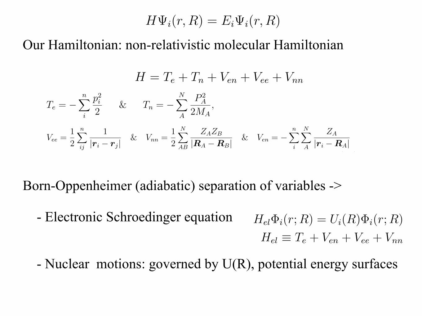
Our Hamiltonian: non-relativistic molecular Hamiltonian
Born-Oppenheimer (adiabatic) separation of variables ->
- Electronic Schroedinger equation
- Nuclear motions: governed by U(R), potential energy surfaces
10 Introduction
Table 1.2: Energy ranges.Process Energy, hartree Experiment
Annihilation 104 elementary particles’ physicsRadioactivity 102 Messbauer, synchrotron,
gamma-electron spectroscopies1 photoelectron spectroscopy
Ionization, electronic excitation, 0.1-0.01 Electronic spectroscopydissociation (bond energy) chemistryMolecular vibrations 10�2-10�3 IR, RamanMolecular rotations 10�4-10�6 Far IR, radiofrequenciesSpin < 10�4 NMR, EPROrientation in molecular solids ultrasound
geometry changes, it can give the same error in vibrational levels, which means thatthe error would be 3 orders of magnitude larger than calculated quantity! That is whyelectronic structure calculation is an art of making balanced approximations whichresult in error cancellation.
1.3 Adiabatic approximation
1.3.1 Potential energy surfaces and the electronic Hamilto-nian
We start from the non-relativistic Schrodinger equation (SE) for the system of nelectrons and N nuclei. Exact many electron, many nuclei problem is described bythe following SE:
H i(r, R) = Ei i(r, R), (1.3)
where r = r1, r2, . . . , rn, R = R1, R2, . . . , RN represent the electron and nuclear coor-dinates, respectively, and
H = Te + Tn + Ven + Vee + Vnn (1.4)
The kinetic energy terms are:
Te = �nX
i
p2i2
& Tn = �NX
A
P 2A
2MA, (1.5)
where p2 = @2
@x2 +@2
@y2 +@2
@z2 = r2 = �.The Coulomb terms are:
Vee =1
2
nX
ij
1
|ri � rj|& Vnn =
1
2
NX
AB
ZAZB
|RA �RB|& Ven = �
nX
i
NX
A
ZA
|ri �RA|(1.6)
1.3 Adiabatic approximation 11
The solution of equation (1.3) yields wave functions that depend on the coordi-nates of all nuclei and all electrons. Intuitively, we feel that nuclear and electronicmotions are very di↵erent, because their masses are very di↵erent, e.g., the protonmass is 3 orders of magnitude larger than the electron mass. If the masses of nucleiwere infinite, equation (1.3) would reduce to the equation for interacting electronsmoving in the potential of fixed nuclei. Each nuclear configuration would producedi↵erent external potential, which means that electronic energies/wavefunction woulddepend on nuclear positions parametrically. We cannot, however, just set up M = 1(i.e., TN = 0), since then we would not be able to describe nuclear dynamics (therewould be no dynamics!). But since the nuclear motion is much slower relative toelectronic motion, we can expect that electrons can adjust almost simultaneously toany new position of nuclei. Let us see how we can separate nuclear and electronicmotion.
Let us define so-called electronic wavefunctions to be solutions of the electronicSE:
Hel�i(r;R) = Ui(R)�i(r;R) (1.7)
Hel ⌘ Te + Ven + Vee + Vnn (1.8)
We can solve this equation at each fixed geometry of nuclei, and resulting solution(U and �) will depend parametrically on nuclear geometry (we use ’;’ instead of ’,’ todistinguish between parametric and explicit dependence on R). Calculated adiabaticpotential energy curves Ui(R) of O2 molecule are shown in Fig. 1.2. We will see laterthat U(R) is a potential which governs nuclear motion (bound states — vibrationalmotion, unbound states — dissociation, etc). At each internuclear distance, the lowestenergy solution of the electronic SE gives ground state energy. Higher energy solutionsdescribe electronically excited states. Note that some of the states are unbound, i.e.,if molecule is excited to one of such states, it dissociates to two oxygen atoms.
Equation (1.8) is the equation of the electronic structure theory. This is what wesolve and this is our “first principle”.
Now we want to express solutions of full problem (1.3) in terms of the solutionsof the electronic problem. We can express the exact wavefunction as:
i(r, R) =X
j
�j(r;R)⇠ij(R) (1.9)
Here functions �j are used as a basis, and so called nuclear functions ⇠ij(R) areexpansion coe�cients to be determined. From now on, we will skip r, R, we will justremember that �j ⌘ �j(r;R) and ⇠ij ⌘ ⇠ij(R).
Now we want to derive equations for so defined ⇠ij. Substitute ansatz (1.9) intoSE (1.3):
(Hel + TN)X
j
�j⇠ij = Ei
X
j
�j⇠ij (1.10)
Multiply this equation by �k on the left, and integrate over the electronic coordinates:
X
j
< �k|Hel|�j >r ⇠ij +
X
j
< �k|TN |�j⇠ij >r= Ei
X
j
< �k|�j >r ⇠ij (1.11)
1.3 Adiabatic approximation 13
Therefore we end up with the following set of equations for ⇠ij:
(TN + Uk(R)� Ei) ⇠ik =
X
A
1
2MA
0
@X
j
< �k|r2A�j >r ⇠
ij + 2
X
j
< �k|rA�j >r rA⇠ij
1
A
(1.15)If we could neglect terms on the right, we would end up with an eigenproblem for
nuclei moving in the potential Uk, which is mean field potential of electrons (electroncloud). For each Uk we can find nuclear eigenstates, and eigenstates for di↵erent Uk
are independent. In this case ansatz (1.9) assumes simpler form:
ik = �i⇠ik (1.16)
We can consider PES’s from Fig. 1.2. For bound states, there will be quantizedvibrational energy levels, and localized nuclear vibrational wavefunctions (similar toharmonic oscillator functions). Solution of the nuclear SE for unbound PES’s willproduce continuum energy levels and wave-like wavefunctions.
In the classical limit, we can consider nuclei as spheres moving on the given poten-tial Uk. Once nuclei are placed on the given Uk, they will stay on this surface forever:electronic state Uk cannot change to Ui upon nuclear motion. In other words, elec-trons can adjust to a new nuclear position simultaneously. They are infinitely fastrelative to nuclei. This is adiabatic (Born-Oppenheimer approximation).
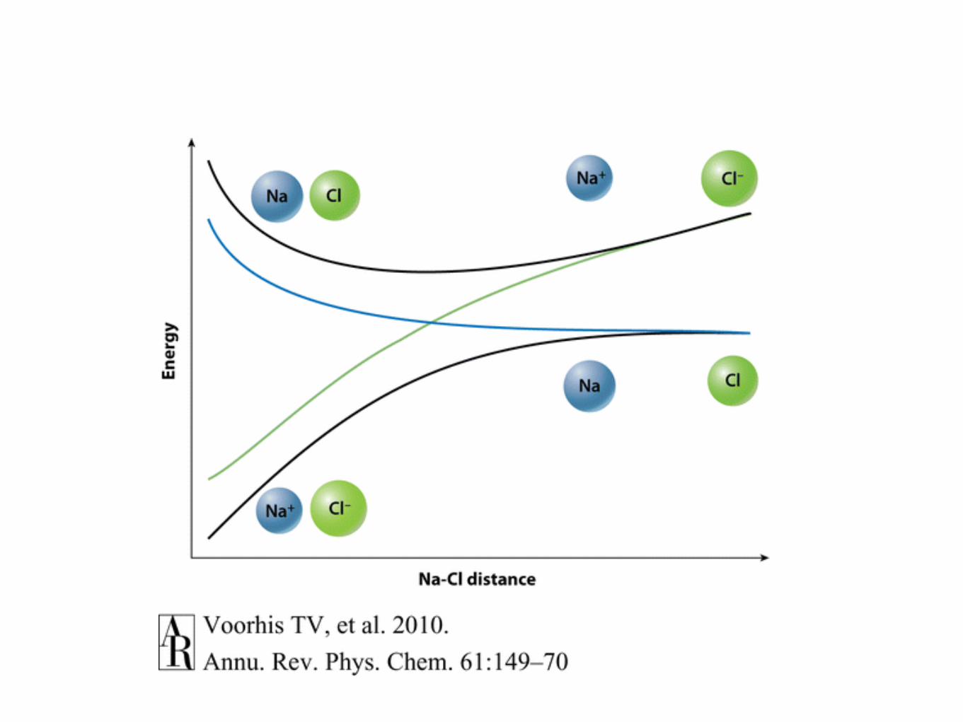
Let us analyze terms on the right. What do they do? Consider their diagonalpart. Some correction to the energy, second is zero. Non-diagonal parts: they couplenuclear dynamics on di↵erent electronic states. Using classical language, due to thisterms electronic state can change upon the nuclear motion — there is a probability ofnon-adiabatic hops. When these terms can be large? When electronic wavefunctiondepend strongly on nuclear geometry (derivative terms)! Fig. 1.3 shows adiabaticPES’s for NaI. At equilibrium, the molecule is ionic. However, lowest energy gas phasedissociation channel is neutral one. Thus, the wavefunction changes its character fromionic to neutral, and the derivative coupling may be large. It is possible to consider socalled diabatic states, states that do not change their nature as a function of nucleargeometry. These states are no longer eigenstates of electronic SE. Thus, they arecoupled by a potential coupling, an o↵-diagonal matrix element of the Hamiltonian inthe basis of diabatic states.
Term < �k|r2A�j >r ⇠ij is just some potential coupling (acts as additional po-
tential for nuclei). To be important, it has to be large relative to diagonal parts ofthe Hamiltonian (potential Uk). So its importance is defined solely by the value ofthe integral < �k|r2
A�j >r and the potentials Uk. TermP
j < �k|rA�j >r rA⇠ij,however, is di↵erent. It has two parts: integral
Pj < �k|rA�j >r, and nuclear mo-
mentum rA⇠ij. Therefore, this term can become very large when nuclear velocity ishigh. Here we can discuss two limits: adiabatic limit: nuclei are very slow, electronsfollow nuclear motion and adjust to it. Nuclear are very fast — electrons cannotadjust to nuclear motion — non-adiabatic “hops”.
As a homework, use PT to analyze termP
j < �k|rA�j >r to understand whenit can be large (see Fig. 1.4).
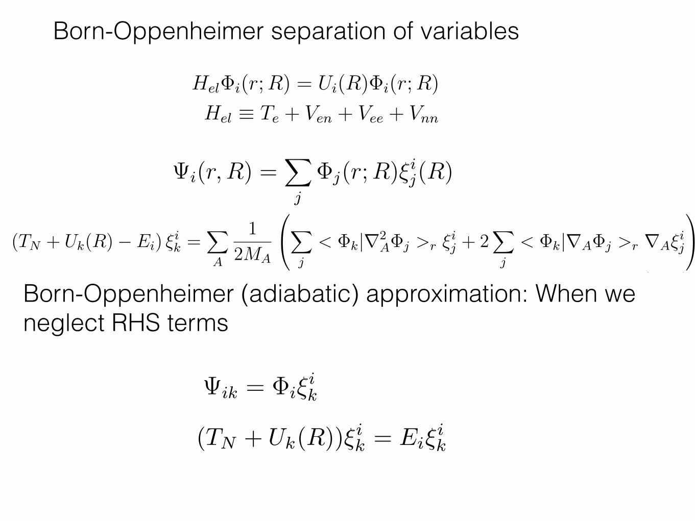
Born-Oppenheimer separation of variables
Born-Oppenheimer (adiabatic) approximation: When we neglect RHS terms
1.3 Adiabatic approximation 13
Therefore we end up with the following set of equations for ⇠ij:
(TN + Uk(R)� Ei) ⇠ik =
X
A
1
2MA
0
@X
j
< �k|r2A�j >r ⇠
ij + 2
X
j
< �k|rA�j >r rA⇠ij
1
A
(1.15)If we could neglect terms on the right, we would end up with an eigenproblem for
nuclei moving in the potential Uk, which is mean field potential of electrons (electroncloud). For each Uk we can find nuclear eigenstates, and eigenstates for di↵erent Uk
are independent. In this case ansatz (1.9) assumes simpler form:
ik = �i⇠ik (1.16)
We can consider PES’s from Fig. 1.2. For bound states, there will be quantizedvibrational energy levels, and localized nuclear vibrational wavefunctions (similar toharmonic oscillator functions). Solution of the nuclear SE for unbound PES’s willproduce continuum energy levels and wave-like wavefunctions.
In the classical limit, we can consider nuclei as spheres moving on the given poten-tial Uk. Once nuclei are placed on the given Uk, they will stay on this surface forever:electronic state Uk cannot change to Ui upon nuclear motion. In other words, elec-trons can adjust to a new nuclear position simultaneously. They are infinitely fastrelative to nuclei. This is adiabatic (Born-Oppenheimer approximation).
Let us analyze terms on the right. What do they do? Consider their diagonalpart. Some correction to the energy, second is zero. Non-diagonal parts: they couplenuclear dynamics on di↵erent electronic states. Using classical language, due to thisterms electronic state can change upon the nuclear motion — there is a probability ofnon-adiabatic hops. When these terms can be large? When electronic wavefunctiondepend strongly on nuclear geometry (derivative terms)! Fig. 1.3 shows adiabaticPES’s for NaI. At equilibrium, the molecule is ionic. However, lowest energy gas phasedissociation channel is neutral one. Thus, the wavefunction changes its character fromionic to neutral, and the derivative coupling may be large. It is possible to consider socalled diabatic states, states that do not change their nature as a function of nucleargeometry. These states are no longer eigenstates of electronic SE. Thus, they arecoupled by a potential coupling, an o↵-diagonal matrix element of the Hamiltonian inthe basis of diabatic states.
Term < �k|r2A�j >r ⇠ij is just some potential coupling (acts as additional po-
tential for nuclei). To be important, it has to be large relative to diagonal parts ofthe Hamiltonian (potential Uk). So its importance is defined solely by the value ofthe integral < �k|r2
A�j >r and the potentials Uk. TermP
j < �k|rA�j >r rA⇠ij,however, is di↵erent. It has two parts: integral
Pj < �k|rA�j >r, and nuclear mo-
mentum rA⇠ij. Therefore, this term can become very large when nuclear velocity ishigh. Here we can discuss two limits: adiabatic limit: nuclei are very slow, electronsfollow nuclear motion and adjust to it. Nuclear are very fast — electrons cannotadjust to nuclear motion — non-adiabatic “hops”.
As a homework, use PT to analyze termP
j < �k|rA�j >r to understand whenit can be large (see Fig. 1.4).
(TN + Uk(R))⇠ik = Ei⇠ik

Potential Energy Surfaces: Concepts and definitions

Cyclobutadiene (C4H4) ring opening: Transition state versus an intermediate

http://www.ch.ic.ac.uk/robb/electron_transfer.php

Stationary points on PES and relation to chemistry


1.3 Adiabatic approximation 11
The solution of equation (1.3) yields wave functions that depend on the coordi-nates of all nuclei and all electrons. Intuitively, we feel that nuclear and electronicmotions are very di↵erent, because their masses are very di↵erent, e.g., the protonmass is 3 orders of magnitude larger than the electron mass. If the masses of nucleiwere infinite, equation (1.3) would reduce to the equation for interacting electronsmoving in the potential of fixed nuclei. Each nuclear configuration would producedi↵erent external potential, which means that electronic energies/wavefunction woulddepend on nuclear positions parametrically. We cannot, however, just set up M = 1(i.e., TN = 0), since then we would not be able to describe nuclear dynamics (therewould be no dynamics!). But since the nuclear motion is much slower relative toelectronic motion, we can expect that electrons can adjust almost simultaneously toany new position of nuclei. Let us see how we can separate nuclear and electronicmotion.
Let us define so-called electronic wavefunctions to be solutions of the electronicSE:
Hel�i(r;R) = Ui(R)�i(r;R) (1.7)
Hel ⌘ Te + Ven + Vee + Vnn (1.8)
We can solve this equation at each fixed geometry of nuclei, and resulting solution(U and �) will depend parametrically on nuclear geometry (we use ’;’ instead of ’,’ todistinguish between parametric and explicit dependence on R). Calculated adiabaticpotential energy curves Ui(R) of O2 molecule are shown in Fig. 1.2. We will see laterthat U(R) is a potential which governs nuclear motion (bound states — vibrationalmotion, unbound states — dissociation, etc). At each internuclear distance, the lowestenergy solution of the electronic SE gives ground state energy. Higher energy solutionsdescribe electronically excited states. Note that some of the states are unbound, i.e.,if molecule is excited to one of such states, it dissociates to two oxygen atoms.
Equation (1.8) is the equation of the electronic structure theory. This is what wesolve and this is our “first principle”.
Now we want to express solutions of full problem (1.3) in terms of the solutionsof the electronic problem. We can express the exact wavefunction as:
i(r, R) =X
j
�j(r;R)⇠ij(R) (1.9)
Here functions �j are used as a basis, and so called nuclear functions ⇠ij(R) areexpansion coe�cients to be determined. From now on, we will skip r, R, we will justremember that �j ⌘ �j(r;R) and ⇠ij ⌘ ⇠ij(R).
Now we want to derive equations for so defined ⇠ij. Substitute ansatz (1.9) intoSE (1.3):
(Hel + TN)X
j
�j⇠ij = Ei
X
j
�j⇠ij (1.10)
Multiply this equation by �k on the left, and integrate over the electronic coordinates:
X
j
< �k|Hel|�j >r ⇠ij +
X
j
< �k|TN |�j⇠ij >r= Ei
X
j
< �k|�j >r ⇠ij (1.11)
1.3 Adiabatic approximation 13
Therefore we end up with the following set of equations for ⇠ij:
(TN + Uk(R)� Ei) ⇠ik =
X
A
1
2MA
0
@X
j
< �k|r2A�j >r ⇠
ij + 2
X
j
< �k|rA�j >r rA⇠ij
1
A
(1.15)If we could neglect terms on the right, we would end up with an eigenproblem for
nuclei moving in the potential Uk, which is mean field potential of electrons (electroncloud). For each Uk we can find nuclear eigenstates, and eigenstates for di↵erent Uk
are independent. In this case ansatz (1.9) assumes simpler form:
ik = �i⇠ik (1.16)
We can consider PES’s from Fig. 1.2. For bound states, there will be quantizedvibrational energy levels, and localized nuclear vibrational wavefunctions (similar toharmonic oscillator functions). Solution of the nuclear SE for unbound PES’s willproduce continuum energy levels and wave-like wavefunctions.
In the classical limit, we can consider nuclei as spheres moving on the given poten-tial Uk. Once nuclei are placed on the given Uk, they will stay on this surface forever:electronic state Uk cannot change to Ui upon nuclear motion. In other words, elec-trons can adjust to a new nuclear position simultaneously. They are infinitely fastrelative to nuclei. This is adiabatic (Born-Oppenheimer approximation).
Let us analyze terms on the right. What do they do? Consider their diagonalpart. Some correction to the energy, second is zero. Non-diagonal parts: they couplenuclear dynamics on di↵erent electronic states. Using classical language, due to thisterms electronic state can change upon the nuclear motion — there is a probability ofnon-adiabatic hops. When these terms can be large? When electronic wavefunctiondepend strongly on nuclear geometry (derivative terms)! Fig. 1.3 shows adiabaticPES’s for NaI. At equilibrium, the molecule is ionic. However, lowest energy gas phasedissociation channel is neutral one. Thus, the wavefunction changes its character fromionic to neutral, and the derivative coupling may be large. It is possible to consider socalled diabatic states, states that do not change their nature as a function of nucleargeometry. These states are no longer eigenstates of electronic SE. Thus, they arecoupled by a potential coupling, an o↵-diagonal matrix element of the Hamiltonian inthe basis of diabatic states.
Term < �k|r2A�j >r ⇠ij is just some potential coupling (acts as additional po-
tential for nuclei). To be important, it has to be large relative to diagonal parts ofthe Hamiltonian (potential Uk). So its importance is defined solely by the value ofthe integral < �k|r2
A�j >r and the potentials Uk. TermP
j < �k|rA�j >r rA⇠ij,however, is di↵erent. It has two parts: integral
Pj < �k|rA�j >r, and nuclear mo-
mentum rA⇠ij. Therefore, this term can become very large when nuclear velocity ishigh. Here we can discuss two limits: adiabatic limit: nuclei are very slow, electronsfollow nuclear motion and adjust to it. Nuclear are very fast — electrons cannotadjust to nuclear motion — non-adiabatic “hops”.
As a homework, use PT to analyze termP
j < �k|rA�j >r to understand whenit can be large (see Fig. 1.4).
Non Born-Oppenheimer case
Non-adiabatic dynamics in which nuclear and electronic motions are coupled. Nuclear motions on multiple surfaces are coupled and there are non-adiabatic transitions

1.3 Adiabatic approximation 13
Therefore we end up with the following set of equations for ⇠ij:
(TN + Uk(R)� Ei) ⇠ik =
X
A
1
2MA
0
@X
j
< �k|r2A�j >r ⇠
ij + 2
X
j
< �k|rA�j >r rA⇠ij
1
A
(1.15)If we could neglect terms on the right, we would end up with an eigenproblem for
nuclei moving in the potential Uk, which is mean field potential of electrons (electroncloud). For each Uk we can find nuclear eigenstates, and eigenstates for di↵erent Uk
are independent. In this case ansatz (1.9) assumes simpler form:
ik = �i⇠ik (1.16)
We can consider PES’s from Fig. 1.2. For bound states, there will be quantizedvibrational energy levels, and localized nuclear vibrational wavefunctions (similar toharmonic oscillator functions). Solution of the nuclear SE for unbound PES’s willproduce continuum energy levels and wave-like wavefunctions.
In the classical limit, we can consider nuclei as spheres moving on the given poten-tial Uk. Once nuclei are placed on the given Uk, they will stay on this surface forever:electronic state Uk cannot change to Ui upon nuclear motion. In other words, elec-trons can adjust to a new nuclear position simultaneously. They are infinitely fastrelative to nuclei. This is adiabatic (Born-Oppenheimer approximation).
Let us analyze terms on the right. What do they do? Consider their diagonalpart. Some correction to the energy, second is zero. Non-diagonal parts: they couplenuclear dynamics on di↵erent electronic states. Using classical language, due to thisterms electronic state can change upon the nuclear motion — there is a probability ofnon-adiabatic hops. When these terms can be large? When electronic wavefunctiondepend strongly on nuclear geometry (derivative terms)! Fig. 1.3 shows adiabaticPES’s for NaI. At equilibrium, the molecule is ionic. However, lowest energy gas phasedissociation channel is neutral one. Thus, the wavefunction changes its character fromionic to neutral, and the derivative coupling may be large. It is possible to consider socalled diabatic states, states that do not change their nature as a function of nucleargeometry. These states are no longer eigenstates of electronic SE. Thus, they arecoupled by a potential coupling, an o↵-diagonal matrix element of the Hamiltonian inthe basis of diabatic states.
Term < �k|r2A�j >r ⇠ij is just some potential coupling (acts as additional po-
tential for nuclei). To be important, it has to be large relative to diagonal parts ofthe Hamiltonian (potential Uk). So its importance is defined solely by the value ofthe integral < �k|r2
A�j >r and the potentials Uk. TermP
j < �k|rA�j >r rA⇠ij,however, is di↵erent. It has two parts: integral
Pj < �k|rA�j >r, and nuclear mo-
mentum rA⇠ij. Therefore, this term can become very large when nuclear velocity ishigh. Here we can discuss two limits: adiabatic limit: nuclei are very slow, electronsfollow nuclear motion and adjust to it. Nuclear are very fast — electrons cannotadjust to nuclear motion — non-adiabatic “hops”.
As a homework, use PT to analyze termP
j < �k|rA�j >r to understand whenit can be large (see Fig. 1.4).

Adiabatic states and wave function evolution: understanding the derivative term
4

Homework: Why non-adiabatic transitions are more likely to occur when the PESs are close?

On the importance of non-adiabatic effects
Barriers differ by 0.4 eV, but the ratio is 1:0.4 in favor of the channel with the HIGHER barrier

Rydberg
Dynamics on multiple surfaces in the NO dimer: Break down of Adiabatic approximation

Stationary points on PES and relation to chemistry


![Adiabatic process..."adiabatic approximation", meaning that there is not enough time for the transfer of energy as heat to take place to or from the system.[3] By way of example, the](https://img.dokumen.tips/doc/110x75/5f252aad3b64b47c6b301a9d/adiabatic-process-adiabatic-approximation-meaning-that-there-is.jpg)
![Averaging of Linear Operators, Adiabatic Approximation ...geomanal...the number of “phases ... The digits over the operators denote the order of action of these operators (see [11])](https://img.dokumen.tips/doc/110x75/5ea62e4e2d20a6550b19f223/averaging-of-linear-operators-adiabatic-approximation-geomanalthe-number.jpg)
![Ulf Lorenz arXiv:1607.01714v2 [quant-ph] 11 Oct 2016 · Born-Oppenheimer (adiabatic) approximation, where the dynamics may be dominated by (avoided) crossings or conical intersections](https://img.dokumen.tips/doc/110x75/603539b581e3ed4b550f8e29/ulf-lorenz-arxiv160701714v2-quant-ph-11-oct-2016-born-oppenheimer-adiabatic.jpg)