Embed Size (px)
Citation preview

12INFINITE SEQUENCES AND SERIESINFINITE SEQUENCES AND SERIES

12.9Representations of
Functions as Power Series
INFINITE SEQUENCES AND SERIES
In this section, we will learn:
How to represent certain functions as
sums of power series.

FUNCTIONS AS POWER SERIES
We can represent certain types
of functions as sums of power series
by either:
Manipulating geometric series
Differentiating or integrating such a series

FUNCTIONS AS POWER SERIES
You might wonder:
Why would we ever want to express a known function as a sum of infinitely many terms?
FUNCTIONS AS POWER SERIES
We will see that this strategy is
useful for:
Integrating functions without elementary antiderivatives
Solving differential equations
Approximating functions by polynomials

FUNCTIONS AS POWER SERIES
Scientists do this to simplify the expressions
they deal with.
Computer scientists do this to represent
functions on calculators and computers.

FUNCTIONS AS POWER SERIES
We start with an equation we have seen
before:
Equation 1
2 3
0
11 ... 1
1n
n
x x x x xx
FUNCTIONS AS POWER SERIES
We first saw this equation in Example 5
in Section 11.2
We obtained it by observing that it is a geometric series with a = 1 and r = x.

FUNCTIONS AS POWER SERIES
However, here our point of view is
different.
We regard Equation 1 as expressing the function f(x) = 1/(1 – x) as a sum of a power series.

FUNCTIONS AS POWER SERIES
A geometric illustration of Equation 1
is shown.
Fig. 12.9.1, p. 764

FUNCTIONS AS POWER SERIES
Since the sum of a series is the limit of
the sequence of partial sums, we have
where sn(x) = 1 + x + x2 + … + xn
is the nth partial sum.
1lim ( )
1 nns x
x

FUNCTIONS AS POWER SERIES
Notice that, as n increases, sn(x)
becomes a better approximation to f(x)
for –1 < x < 1.
Fig. 12.9.1, p. 764
FUNCTIONS AS POWER SERIES
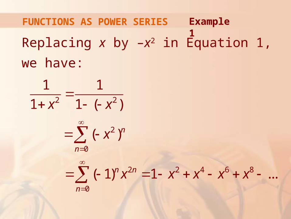
Express 1/(1 + x2) as the sum of
a power series and find the interval of
convergence.
Example 1
FUNCTIONS AS POWER SERIES
Replacing x by –x2 in Equation 1,
we have:
2 2
2
0
2 2 4 6 8
0
1 1
1 1 ( )
( )
( 1) 1 ...
n
n
n n
n
x x
x
x x x x x
Example 1
FUNCTIONS AS POWER SERIES
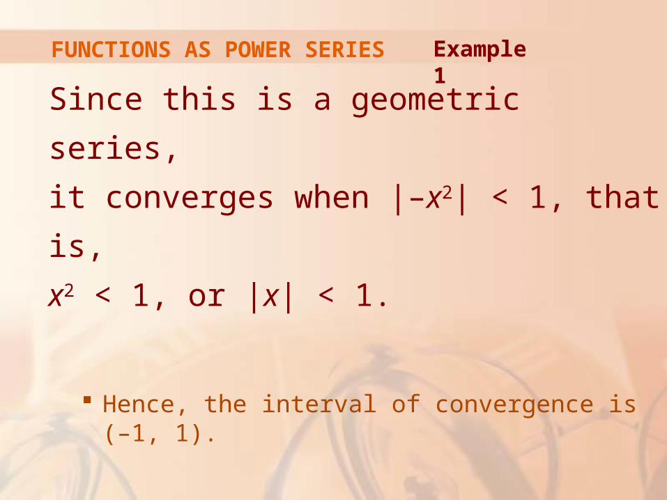
Since this is a geometric series,
it converges when |–x2| < 1, that is,
x2 < 1, or |x| < 1.
Hence, the interval of convergence is (–1, 1).
Example 1
FUNCTIONS AS POWER SERIES
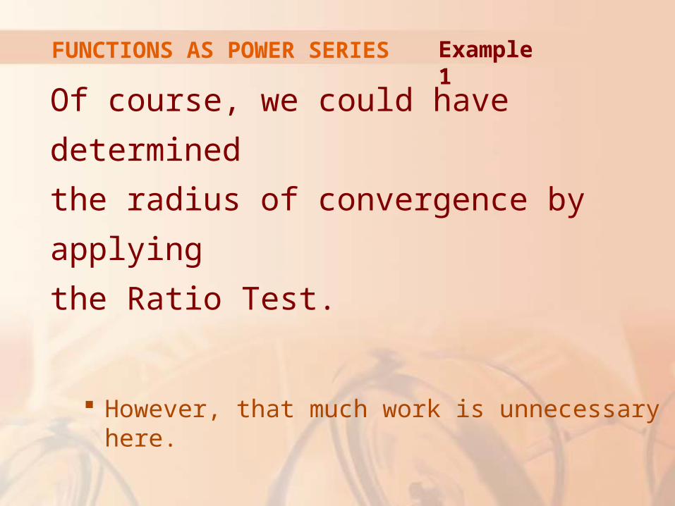
Of course, we could have determined
the radius of convergence by applying
the Ratio Test.
However, that much work is unnecessary here.
Example 1

FUNCTIONS AS POWER SERIES
Find a power series representation
for 1/(x + 2).
We need to put this function in the form of the left side of Equation 1.
Example 2

FUNCTIONS AS POWER SERIES
So, we first factor a 2 from the denominator:
0
10
1 1 1
2 2 1 2 12 2
1
2 2
( 1)
2
n
n
nn
nn
xx x
x
x
Example 2

FUNCTIONS AS POWER SERIES
This series converges when |–x/2| < 1,
that is, |x| < 2.
So, the interval of convergence is (–2, 2).
Example 2

FUNCTIONS AS POWER SERIES
Find a power series representation
of x3/(x + 2).
This function is just x3 times the function in Example 2.
So, all we have to do is multiply that series by x3, as follows.
Example 3
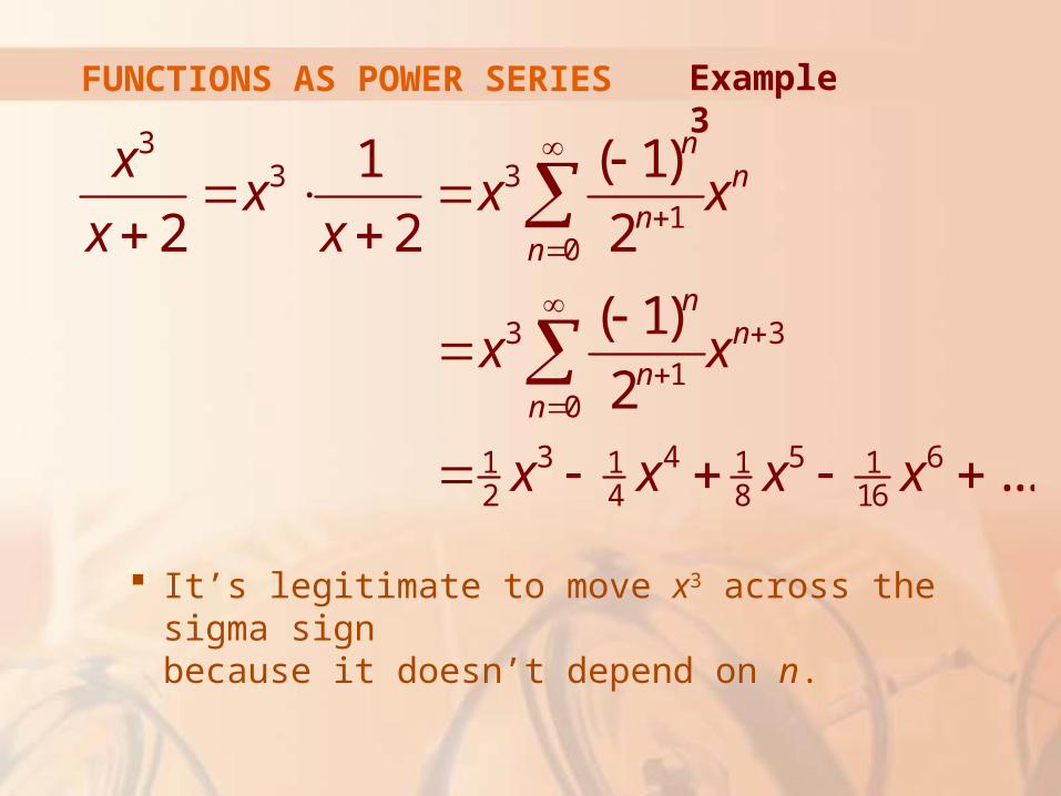
FUNCTIONS AS POWER SERIES
It’s legitimate to move x3 across the sigma sign because it doesn’t depend on n.
33 3
10
3 31
0
3 4 5 61 1 1 12 4 8 16
1 ( 1)
2 2 2
( 1)
2
...
nn
nn
nn
nn
xx x x
x x
x x
x x x x
Example 3

FUNCTIONS AS POWER SERIES
Another way of writing this series is:
As in Example 2, the interval of convergence is (–2, 2).
3 1
23
( 1)
2 2
nn
nn
xx
x
Example 3

DIFFERENTIATION & INTEGRATION OF POWER SERIES
The sum of a power series is a function
whose domain is the interval of convergence
of the series.
We would like to be able to differentiate and integrate such functions.
0
( ) ( )nnn
f x c x a

TERM–BY–TERM DIFFN. & INTGN.
The following theorem (which we won’t prove)
says that we can do so by differentiating or
integrating each individual term in the series—
just as we would for a polynomial.
This is called term-by-term differentiation and integration.

TERM–BY–TERM DIFFN. & INTGN.
If the power series Σ cn(x – a)n has radius of
convergence R > 0, the function f defined by
is differentiable (and therefore continuous) on
the interval (a – R, a + R).
20 1 2
0
( ) ( ) ( ) ...
( )nnn
f x c c x a c x a
c x a
Theorem 2

TERM–BY–TERM DIFFN. & INTGN.
Also,
i.
ii.
The radii of convergence of the power series in Equations i and ii are both R.
21 2 3
1
1
'( ) 2 ( ) 3 ( ) ...
( )nnn
f x c c x a c x a
nc x a
2 3
0 1 2
1
0
( ) ( )( ) ( ) ...
2 3
( )
1
nn
n
x a x af x dx C c x a c c
c x aC
n
Theorem 2

TERM–BY–TERM DIFFN. & INTGN.
In part ii, ∫ c0 dx = c0x + C1 is written as
c0(x – a) + C, where C = C1 + ac0.
So, all the terms of the series have the same form.

NOTE 1
Equations i and ii in Theorem 2 can be
rewritten in the form
iii.
iv.
0 0
( ) ( )n nn n
n n
d dc x a c x a
dx dx
0 0
( ) ( )n nn n
n n
c x a dx c x a dx

NOTE 1
For finite sums, we know that:
The derivative of a sum is the sum of the derivatives.
The integral of a sum is the sum of the integrals.

NOTE 1
Equations iii and iv assert that the same
is true for infinite sums—provided we are
dealing with power series.
For other types of series of functions, the situation is not as simple (see Exercise 36).
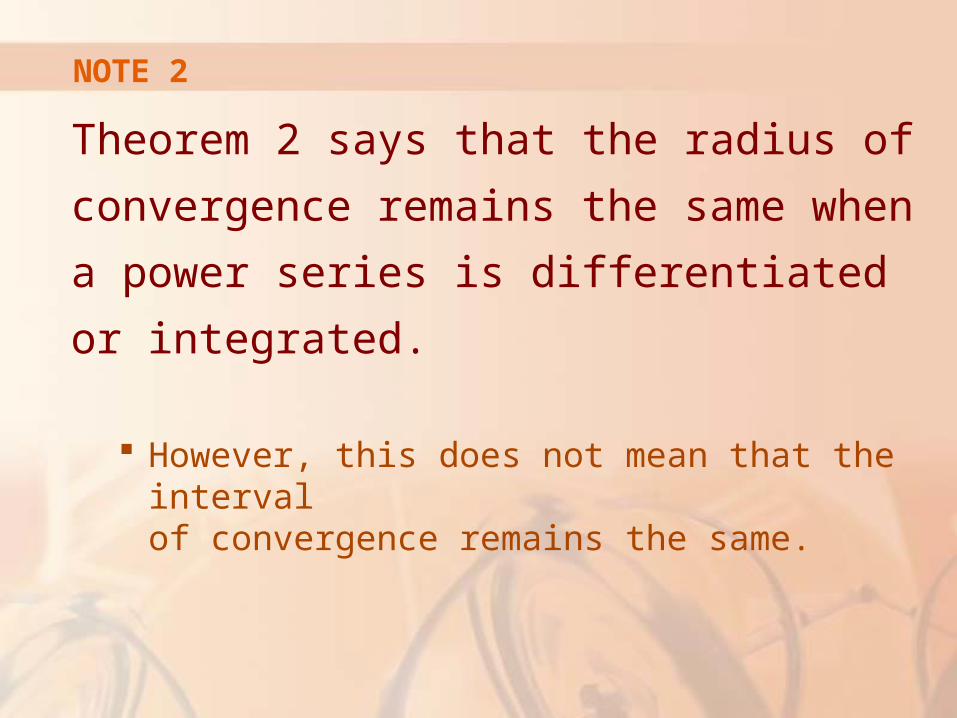
NOTE 2
Theorem 2 says that the radius of
convergence remains the same when a power
series is differentiated or integrated.
However, this does not mean that the interval of convergence remains the same.

NOTE 2
It may happen that the original series
converges at an endpoint, whereas
the differentiated series diverges there.
See Exercise 37.

NOTE 3
The idea of differentiating a power series
term by term is the basis for a powerful
method for solving differential equations.
We will discuss this method in Chapter 17.

TERM–BY–TERM DIFFN. & INTGN.
In Example 3 in Section 11.8, we saw that
the Bessel function
is defined for all x.
Example 4
2
0 2 20
( 1)( )
2 ( !)
n n
nn
xJ x
n

TERM–BY–TERM DIFFN. & INTGN.
Thus, by Theorem 2, J0 is differentiable for
all x and its derivative is found by term-by-
term differentiation as follows:
2
0 2 20
2 1
2 20
( 1)'( )
2 ( !)
( 1) 2
2 ( !)
n n
nn
n n
nn
d xJ x
dx n
n x
n
Example 4

TERM–BY–TERM DIFFN. & INTGN.
Express 1/(1 – x)2 as a power series by
differentiating Equation 1.
What is the radius of convergence?
Example 5

TERM–BY–TERM DIFFN. & INTGN.
Differentiating each side of the equation
we get:
2 3
0
11 ...
1n
n
x x x xx
2 12
1
11 2 3 ...
(1 )n
n
x x nxx
Example 5
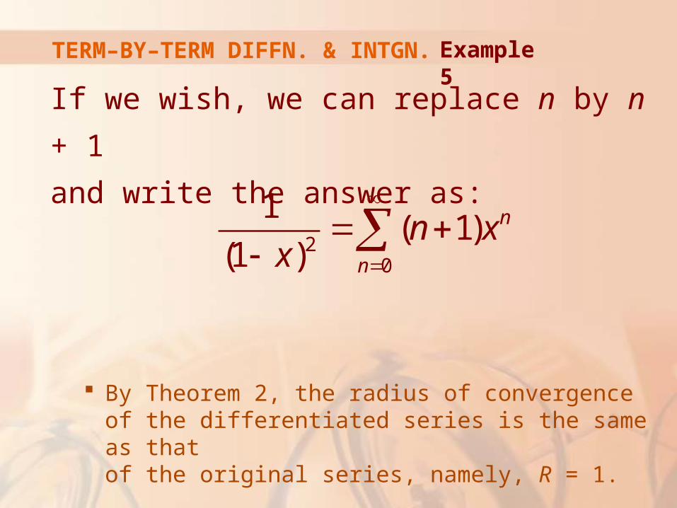
TERM–BY–TERM DIFFN. & INTGN.
If we wish, we can replace n by n + 1
and write the answer as:
By Theorem 2, the radius of convergence of the differentiated series is the same as that of the original series, namely, R = 1.
20
1( 1)
(1 )n
n
n xx
Example 5
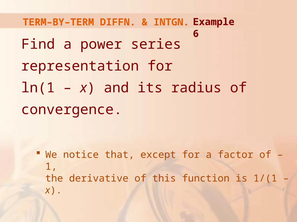
TERM–BY–TERM DIFFN. & INTGN.
Find a power series representation for
ln(1 – x) and its radius of convergence.
We notice that, except for a factor of –1, the derivative of this function is 1/(1 – x).
Example 6

TERM–BY–TERM DIFFN. & INTGN.
So, we integrate both sides of Equation 1:
2
2 3
1
0 1
1ln(1 )
1
(1 ...)
...2 3
11
n n
n n
x dxx
x x dx
x xx C
x xC C x
n n
Example 6

TERM–BY–TERM DIFFN. & INTGN.
To determine the value of C, we put x = 0
in this equation and obtain –ln(1 – 0) = C.
Thus, C = 0 and
The radius of convergence is the same as for the original series: R = 1.
2 3
1
ln(1 ) ... 12 3
n
n
x x xx x x
n
Example 6

TERM–BY–TERM DIFFN. & INTGN.
Notice what happens if we put x = ½
in the result of Example 6.
Since ln ½ = -ln 2, we see that:
1
1 1 1 1 1ln 2 ...
2 8 24 64 2nn n
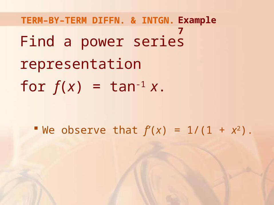
TERM–BY–TERM DIFFN. & INTGN.
Find a power series representation
for f(x) = tan-1 x.
We observe that f’(x) = 1/(1 + x2).
Example 7

TERM–BY–TERM DIFFN. & INTGN.
Thus, we find the required series by integrating the power series for 1/(1 + x2) found in Example 1.
12
2 4 6
3 5 7
1tan
1
(1 ...)
...3 5 7
x dxx
x x x dx
x x xC x
Example 7

TERM–BY–TERM DIFFN. & INTGN.
To find C, we put x = 0 and obtain C = tan-1 0.
Hence,
Since the radius of convergence of the series for 1/(1 + x2) is 1, the radius of convergence of this series for tan-1 x is also 1.
3 5 7 2 11
0
tan ... ( 1)3 5 7 2 1
nn
n
x x x xx x
n
Example 7

GREGORY’S SERIES
The power series for tan-1x obtained in
Example 7 is called Gregory’s series.
It is named after the Scottish mathematician James Gregory (1638–1675), who had anticipated some of Newton’s discoveries.

GREGORY’S SERIES
We have shown that Gregory’s series
is valid when –1 < x < 1.
However, it turns out that it is also valid when x = ±1.
This isn’t easy to prove, though.

GREGORY’S SERIES
Notice that, when x = 1, the series
becomes:
This beautiful result is known as the Leibniz formula for π.
1 1 11 ...
4 3 5 7

TERM–BY–TERM DIFFN. & INTGN.
a. Evaluate ∫ [1/(1 + x7)] dx as a power series.
b. Use part (a) to approximate
correct to within 10–7.
Example 8
0.5 7
0[1/(1 )]x dx

TERM–BY–TERM DIFFN. & INTGN.
The first step is to express the integrand,
1/(1 + x7), as the sum of a power series.
As in Example 1, we start with Equation 1 and replace x by –x7:
Example 8 a
77 7
0
7
0
7 14
1 1( )
1 1 ( )
( 1)
1 ...
n
n
nn
n
xx x
x
x x

TERM–BY–TERM DIFFN. & INTGN.
Now, we integrate term by term:
This series converges for |–x7| < 1, that is, for |x| < 1.
72
0
7 1
0
8 15 22
1( 1)
1
( 1)7 1
...8 15 22
n n
n
nn
n
dx x dxx
xC
n
x x xC x
Example 8 a

TERM–BY–TERM DIFFN. & INTGN.
In applying the Fundamental Theorem
of Calculus (FTC), it doesn’t matter which
antiderivative we use.
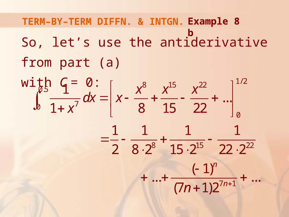
Example 8 b
TERM–BY–TERM DIFFN. & INTGN.
So, let’s use the antiderivative from part (a)
with C = 0:
Example 8 b
1/ 28 15 220.5
700
8 15 22
7 1
1...
1 8 15 22
1 1 1 1
2 8 2 15 2 22 2
( 1)... ...
(7 1)2
n
n
x x xdx x
x
n

TERM–BY–TERM DIFFN. & INTGN.
This infinite series is the exact value of
the definite integral.
However, since it is an alternating series,
we can approximate the sum using the
Alternating Series Estimation Theorem.
Example 8 b

TERM–BY–TERM DIFFN. & INTGN.
If we stop adding after the term
with n = 3, the error is smaller than
the term with n = 4:
Example 8 b
1129
16.4 10
29 2

TERM–BY–TERM DIFFN. & INTGN.
So, we have:
0.5
70
8 15 22
1
11 1 1 1
2 8 2 15 2 22 20.49951374
dxx

TERM–BY–TERM DIFFN. & INTGN.
This example demonstrates one way
in which power series representations
are useful.
Integrating 1/(1 + x7) by hand is incredibly difficult.
Different computer algebra systems (CAS) return different forms of the answer, but they are all extremely complicated.
TERM–BY–TERM DIFFN. & INTGN.
The infinite series answer that we obtain
in Example 8 a is actually much easier
to deal with than the finite answer provided
by a CAS.