NATIONAL INSTITUTE OF TECHNOLOGY, ROURKELA

REALTIME

CLASSIFICATION OF ECG

WAVEFORMS FOR

DIAGNOSIS OF DISEASES

By

Soumya Ranjan Mishra

And

K Goutham

Under the supervision of

Dr. Dipti Patra

Electrical Engineering

NIT Rourkela

2009-2010

REALTIMECLASSIFICATIONOF

ELECTROCARDIOGRAMWAVEFORMS

FORDIAGNOSISOFDISEASES

ATHESISSUBMITTEDINPARTIALFULFILLMENTOFTHEREQUIREMENTS

FORTHEDEGREEOF

BachelorofTechnology

In

ElectricalEngineering

By Soumya Ranjan Mishra

& K. Goutham

Under the supervision of Dr. Dipti Patra

Electrical Engineering NIT Rourkela

Department Of Electrical

Engineering

NIT Rourkela

National Institute Of Technology

Rourkela

CERTIFICATECERTIFICATECERTIFICATECERTIFICATE

This is to certify that the thesis entitled, ”real-time classification of ECG

signals for diagnosis of diseases” by Soumya Ranjan Mishra and K Goutham

in partial requirements for the curriculum requirement of Bachelor of

technology in Electrical Engineering at National Institute Of Technology,

Rourkela, is an authentic work carried out by them under my supervision and

guidance.

To the best of my knowledge, the matter embodied in the thesis has not been

submitted to any other University/Institute for the award of any degree.

Date: Dr. Dipti Patra

Electrical Engineering

NIT, Rourkela

CONTENTS

1. Abstract ………………………………….……………….………01

2. Introduction ………………………………………….………….02

3. Background ……………………………………….……….……..04

3.1. The Electrocardiogram………………….……….……….04

4. Material and methods……………………….………….…………07

4.1. The wavelet transform………..……….………………….07

4.2. The Daubechies wavelet transform……………………….08

4.3. Multilayered Perceptron based Neural Network………….12

5. Results and inference…………..………………………………….14

5.1. Wavelet decomposition…………………………………..14

5.2. Neural networks………………………………………….17

6. SIMULINK model implementation………………………………19

6.1. SIMULINK results…………………………..…………..22

7. Conclusion and future work……………...……………………….23

8. References…………………………………………….…………..24

ACKNOWLEDGEMENT

We would like to express our sincere gratitude towards our teacher and

guide, Dr. Dipti Patra who infused us with the drive to carry on the project

work by her consistent support and encouragement throughout the project

work. Without her support, the thesis would have never been completed.

We would like to thank the faculty of Electrical Engineering department of

NIT, Rourkela for being the panacea to all our queries.

Last but not the least, we would like to thank all our dear friends for being

their wikipediaic knowledge and unrelenting support.

Regards,

Soumya Ranjan Mishra

K Goutham

1 | 2 0 1 0

ABSTRACT

Signal Processing is undoubtedly the best real time implementation of a specific

problem. Wavelet Transform is a very powerful technique for feature extraction and can be used

along with neural network structures to build computationally efficient models for diagnosis of

Biosignals (ECG in this case). This work utilises the above techniques for diagnosis of an ECG

signal by determining its nature as well as exploring the possibility for real-time implementation

of the above model. Daubechies wavelet transform and multi-layered perceptron are the

computational techniques used for the realisation of the above model. The ECG signals were

obtained from the MIT-BIH arrhythmia database and are used for the identification of four

different types of arrythmias. The identification was implemented real-time in SIMULINK, to

simulate the detection model under test condition and verify its workability.

2 | 2 0 1 0

INTRODUCTION

Electrocardiography deals with the electrical activity of the heart. Monitored by

placing sensors at limb extremities of the subject, the electrocardiogram (ECG) is a record of

the origin and propagation of electrical potential through cardiac muscles. It is considered a

representative signal of cardiac physiology, useful in diagnosing cardiac disorders. [Acharya,

Dua, Bhat, Iyengar, Roo,2002];[Owoski and Linh, 2001]; [Ceylan and Ozbay, 2007].

The medical state of the heart is determined by the shape of the Electrocardiogram,

which contains important pointers to different types of diseases afflicting the heart.

However, the electrocardiogram signals are irregular in nature and occur randomly at

different time intervals during a day. Thus arises the need for continuous monitoring of the

ECG signals, which by nature are complex to comprehend and hence there is a possibility of

the analyst missing vital information which can be crucial in determining the nature of the

disease. Thus computer based automated analysis is recommended for early and accurate

diagnosis. [Acharya, Roo, Dua, Iyengar, Bhat, 2002]

The biggest challenge faced by the models for automatic heart beat classification is

the variability of the ECG waveforms from one patient to another even within the same

person. However, different types of arrhythmias have certain characteristics which are

common among all the patients. Thus the objective of a heart beat classifier is to identify

those characteristics so that the diagnosis can be general and as reliable as possible. One of

such methods which can be reliably used for ECG classification is the use of neural

networks. Neural networks are one of the most efficient pattern recognition tools because of

their high nonlinear structure and tendency to minimise error in test inputs by adapting

itself to the input output pattern and thus establishing a nonlinear relationship between the

input and output.

However the performance of a neural network is highly dependent on the number of

3 | 2 0 1 0

input elements in the computational layers.

A large number of elements would lead to a large number of multiplication and

additions and the network would become expensive on computing resources.

Thus to reduce the number of inputs a pre-processing layer is used. This pre-

processor uses wavelet transform to "smooth" out the ECG waveforms and reduce the

number of samples while preserving all the distinct signal features such as local maxima and

minima. Also the use of wavelet transform makes the model to be implemented easily in real

time processing by the use of FIR filters.

The model so obtained was implemented in a real-time model which was simulated

with Simulink software package. The basic processing strategy is shown below. Each bock

represents a processing milestone. The first block is the pre-processor which was described

previously and the second block is the neural network block which does the actual

processing.

DISCRETE

WAVELET

TRANSFORM

MULTILAYERED

PERCEPTRON INPUT DIAGNOSIS

Fig. 1.1 general processing architecture

4 | 2 0 1 0

BACKGROUND

1. The Electrocardiogram:

Electrocardiography (ECG) is a transthoracic interpretation of the electrical

activity of the heart over time captured and externally recorded by skin electrodes.

[ECG simplified by Ashwin Kumar]. The ECG works by detecting and amplifying the

tiny electrical changes on the skin that are caused when the heart muscle "depolarises"

during each heartbeat. At rest, each heart muscle cell has a charge across its outer wall,

or cell membrane. Reducing this charge towards zero is called de-polarisation, which

activates the mechanisms in the cell that cause it to contract. During each heartbeat a

healthy heart will have an orderly progression of a wave of depolarisation that is

triggered by the cells in the sinoatrial node, spreads out through the atrium, passes

through "intrinsic conduction pathways" and then spreads all over the ventricles. This is

detected as tiny rises and falls in the voltage between two electrodes placed either side of

the heart which is displayed as a wavy line either on a screen or on paper. This display

indicates the overall rhythm of the heart and weaknesses in different parts of the heart

muscle.

Usually more than 2 electrodes are used and they can be combined into a

number of pairs. (For example: Left arm (LA), right arm (RA) and left leg (LL)

electrodes form the pairs: LA+RA, LA+LL, RA+LL) The output from each pair is

known as a lead. Each lead is said to look at the heart from a different angle. Different

types of ECGs can be referred to by the number of leads that are recorded, for example

3-lead, 5-lead or 12-lead ECGs (sometimes simply "a 12-lead"). A 12-lead ECG is one

in which 12 different electrical signals are recorded at approximately the same time and

will often be used as a one-off recording of an ECG, typically printed out as a paper

copy. 3- and 5-lead ECGs tend to be monitored continuously and viewed only on the

screen of an appropriate monitoring device, for example during an operation or whilst

being transported in an ambulance. There may, or may not be any permanent record of

5 | 2 0 1 0

a 3- or 5-lead ECG depending on the equipment used.

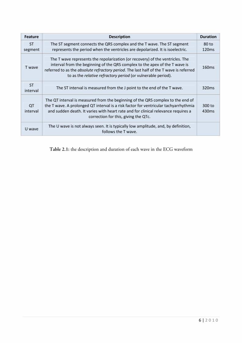
The ECG waveform is shown in the figure 2.1here. The ECG waveform can be

broken down into three important parts each denoting a peak on the either side

represented by P, Q, R, S, T. each of them

represent a vital processes in the heart and

those processes have been illustrated in table

2.1. In case of a disease afflicting the heart,

the waves get distorted according to the area

which is not functioning normally. Thus by

inspection of the ECG waveform the nature

of disease can be found out easily.

TABLE 2.1

Feature Description Duration

RR

interval

The interval between an R wave and the next R wave is the inverse of the heart

rate. Normal resting heart rate is between 50 and 100 bpm

0.6 to

1.2s

P wave

During normal atrial depolarization, the main electrical vector is directed from

the SA node towards the AV node, and spreads from the right atrium to the left

atrium. This turns into the P wave on the ECG.

80ms

PR

interval

The PR interval is measured from the beginning of the P wave to the beginning

of the QRS complex. The PR interval reflects the time the electrical impulse

takes to travel from the sinus node through the AV node and entering the

ventricles. The PR interval is therefore a good estimate of AV node function.

120 to

200ms

PR

segment

The PR segment connects the P wave and the QRS complex. This coincides with

the electrical conduction from the AV node to the bundle of His to the bundle

branches and then to the Purkinje Fibers. This electrical activity does not

produce a contraction directly and is merely traveling down towards the

ventricles and this shows up flat on the ECG. The PR interval is more clinically

relevant.

50 to

120ms

QRS

complex

The QRS complex reflects the rapid depolarization of the right and left

ventricles. They have a large muscle mass compared to the atria and so the QRS

complex usually has a much larger amplitude than the P-wave.

80 to

120ms

J-point The point at which the QRS complex finishes and the ST segment begins. Used

to measure the degree of ST elevation or depression present. N/A

6 | 2 0 1 0

Feature Description Duration

ST

segment

The ST segment connects the QRS complex and the T wave. The ST segment

represents the period when the ventricles are depolarized. It is isoelectric.

80 to

120ms

T wave

The T wave represents the repolarization (or recovery) of the ventricles. The

interval from the beginning of the QRS complex to the apex of the T wave is

referred to as the absolute refractory period. The last half of the T wave is referred

to as the relative refractory period (or vulnerable period).

160ms

ST

interval The ST interval is measured from the J point to the end of the T wave. 320ms

QT

interval

The QT interval is measured from the beginning of the QRS complex to the end of

the T wave. A prolonged QT interval is a risk factor for ventricular tachyarrhythmia

and sudden death. It varies with heart rate and for clinical relevance requires a

correction for this, giving the QTc.

300 to

430ms

U wave The U wave is not always seen. It is typically low amplitude, and, by definition,

follows the T wave.

Table 2.1: the description and duration of each wave in the ECG waveform

7 | 2 0 1 0

MATERIAL AND METHODS

For efficient recognition and less computationally expensive method of pattern

recognition the multi-layered perceptron based neural network is used here along with

wavelet compression of the input signal.

The preclassification task is performed by performing wavelet compression which

reduces the number of samples by a factor of 4.The multi-layered perceptron based neural

network is sued for further processing and final pattern classification.

The input data is clustered as a result of training of the neural network. In the end

a SIMULINK model was developed and it implemented all the result obtained in the

offline analysis. SIMULINK model helped in developing a scheme for real time

implementation of the above process.

The Wavelet Transform

Frequency spectrum analysis is one of the best methods for analysis of a signal.

However Fourier analysis of the signal can decompose the signal into sinusoidal entities

and the filters implementing it remove certain frequencies from the spectrum. However,

this might not be useful in preserving the peaks(local maxima and minima) of the signal

and may lead to loss of important data pointers which are crucial to diagnosis of the

condition.

However, if wavelet transform based data compression is used the peaks (as well as

gaps, though they are not important in this case) can be preserved. This will preserve the

important pointer and structures in the signal. The wavelet transform can be seen as an

extension to the Fourier transform save it works on a multiscale basis unlike Fourier

transform which works on a single domain(frequency domain).The multiscale structure

of the wavelet transform decomposes the signal into a number of scales, each scale

representing a particular coarseness under study.[Ceylan and Ozbay ,2007].

8 | 2 0 1 0

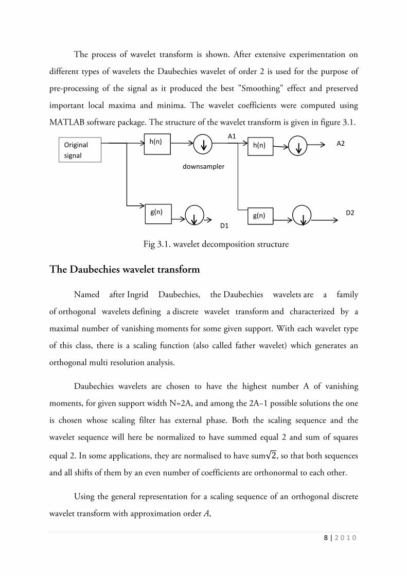
The process of wavelet transform is shown. After extensive experimentation on

different types of wavelets the Daubechies wavelet of order 2 is used for the purpose of

pre-processing of the signal as it produced the best "Smoothing" effect and preserved

important local maxima and minima. The wavelet coefficients were computed using

MATLAB software package. The structure of the wavelet transform is given in figure 3.1.

Fig 3.1. wavelet decomposition structure

The Daubechies wavelet transform

Named after Ingrid Daubechies, the Daubechies wavelets are a family

of orthogonal wavelets defining a discrete wavelet transform and characterized by a

maximal number of vanishing moments for some given support. With each wavelet type

of this class, there is a scaling function (also called father wavelet) which generates an

orthogonal multi resolution analysis.

Daubechies wavelets are chosen to have the highest number A of vanishing

moments, for given support width N=2A, and among the 2A−1 possible solutions the one

is chosen whose scaling filter has external phase. Both the scaling sequence and the

wavelet sequence will here be normalized to have summed equal 2 and sum of squares

equal 2. In some applications, they are normalised to have sum√2, so that both sequences and all shifts of them by an even number of coefficients are orthonormal to each other.

Using the general representation for a scaling sequence of an orthogonal discrete

wavelet transform with approximation order A,

h(n)

g(n)

h(n)

g(n)

Original

signal

downsampler

A1 A2

D1

D2

9 | 2 0 1 0

a(Z) = 21-A(1+Z)Ap(Z), with N=2A, p having real coefficients, p (1) =1 and degree ( p) =A-1, one can

write the orthogonality condition as

�(�)�(�) + �(���)�(−���) = 4

OR

(2 − �)��(�) + ���(2 − �) = 2� , …..(1)

with the Laurent-polynomial � = �� (2 − � − ���) generating all symmetric

sequences and �(−�) = 2 − �(�). Further, P(X) stands for the symmetric Laurent-

polynomial P(X(Z)) = p(Z)p(Z − 1).

Since X(eiw) = 1 − cos(w) and p(eiw)p(e − iw) = | p(eiw) | 2, P takes nonnegative values on the segment [0,2]. Equation (1) has one minimal solution for

each A, which can be obtained by division in the ring of truncated power series in X,.

�#(�) = $ %& + ' − 1& − 1 (

���

)*+2�)��)

Obviously, this has positive values on (0,2)

The homogeneous equation for (1) is antisymmetric about X=1 and has thus the

general solution XA(X − 1)R((X − 1)2), with R some polynomial with real coefficients.

That the sum

P(X) = PA(X) + XA(X − 1)R((X − 1)2) shall be nonnegative on the interval [0,2] translates into a set of linear restrictions

on the coefficients of R. The values of P on the interval [0,2] are bounded by some

quantity 4A − r, maximizing r results in a linear program with infinitely many inequality

conditions.

10 | 2 0 1 0

To solve P(X(Z)) = p(Z)p(Z − 1) for p one uses a technique called spectral factorization resp. Fejer-Riesz-algorithm. The polynomial P(X) splits into linear factors

�(�) = (� − -�) … (� − -/), where N=A+1+2deg(R).

Each linear factor represents a Laurent-polynomial

�(�) − - = − 12 � + 1 − - − 1

2 ���

that can be factored into two linear factors. One can assign either one of the two

linear factors to p (Z), thus one obtains 2N possible solutions. For external phase one

chooses the one that has all complex roots of p(Z) inside or on the unit circle and is thus

real.

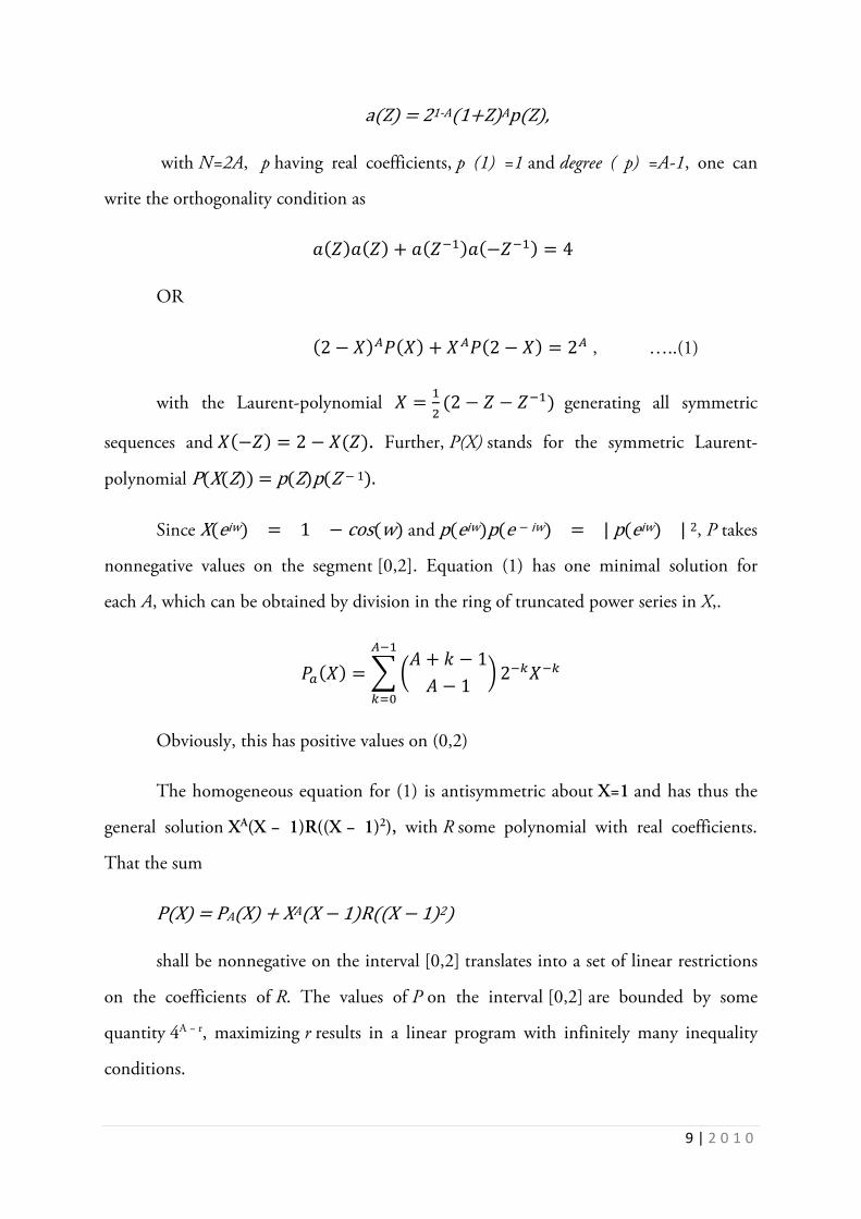
Different orders of Daubechies wavelet transforms are shown below

Fig 3.2:Daubechies wavelet of order 2

11 | 2 0 1 0

Fig 3.3:Daubechies wavelet of order 3

Fig 3.4:Daubechies wavelet of order 4

12 | 2 0 1 0

Multilayered Perceptron based Neural Network

Neural Networks today are synonymous with pattern recognition. The parallel

processing and non-linear architecture make them ideal for finding relationship between

the input and output through various adaptive algorithms. The type of neural network

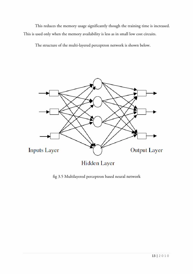
model used here is Multilayer Perceptron based. There are three layers namely the input,

output and the hidden layer having 52, 3 and 10 elements respectively. Each element in

the hidden and the output layer is fully connected to the elements in the input and

hidden layer respectively.

Back propagation algorithm utilises the Levenberg-Marquardt algorithm for

training of the network. It is a quasi-Newton method and is designed to approach the

second order training speed without having to compute the Hessian matrix. When the

performing function has a form of squares (as in typical feed forward networks).The

Hessian matrix can be approximated as H = J5J and gradient computed as G = J57. J is Jacobian matrix containing first derivatives of network errors with respect to weights and

biases. Levenberg-Marquardt algorithm uses the following learning rule.

8)9� = 8) − :;<; + -=>��;<7

Where µ is the gradient descent.

The main advantage of the Levenberg-Marquardt algorithm is the very fast

training. For instance, in this work during the offline analysis the network was seen to

train within 70 epochs. However the algorithm is very resource expensive and uses a large

amount of memory. To reduce the memory usage, a modification is made to the

algorithm by modifying the generation of the Hessian matrix performed by the formula

given below.

? = ;<; = :;�< ;�<> @;�;�A = ;�<;� + ;�<;�

13 | 2 0 1 0

This reduces the memory usage significantly though the training time is increased.

This is used only when the memory availability is less as in small low cost circuits.

The structure of the multi-layered perceptron network is shown below.

fig 3.5 Multilayered perceptron based neural network

14 | 2 0 1 0

RESULTS AND INFERENCE

1. Wavelet decomposition

The objective of this analysis was to determine the wavelet that produces result that is the

closest to the original signal. Different types of wavelet analysis are shown below.

a. Daubechies decomposition of order 1 (Same as Harr wavelet decomposition):

The stages of wavelet decomposition using Daubechies wavelet of order 1 is as follows

the transform was performed on the first 250 samples

Fig 4.1 wavelet decomposition using Daubechies wavelet of order 1

15 | 2 0 1 0

Inference: this wavelet decomposition provides a step output and on higher levels of

decomposition, the signal loses its identity, as the peaks are lost. Thus, this signal is unfit for

use in neural networks.

b. Daubechies wavelet of order 2: As in the former case, this wavelet decomposition

also considers first 250 samples and the results from decomposition are shown below.

Fig 4.2 : wavelet decomposition of second order up to level 3

Inference: The result obtained here can be seen to be smoothed until the second level of

the wavelet transform. After the second level of transform, the signal becomes distorted.

16 | 2 0 1 0

Two level wavelet transform is more apt for processing as the best smoothing can be

achieved with 2 levels without sacrificing accuracy. The number of samples is reduced to

one-fourth of the initial number of samples.

C. Daubechies wavelet decomposition of order 3: As in the former case, this wavelet

decomposition also takes first 250 samples into account and the results from

decomposition are shown below.

Fig 4.1 wavelet decomposition using Daubechies wavelet of order 1

Inference: this decomposition leads to a large deviation from original hence not

recommended for further processing.

17 | 2 0 1 0

Note: Higher order wavelet decomposition produces more deviation and was not taken into

account for further processing. Thus, the second order Daubechies wavelet transform was

used for further processing in the neural network.

2. Neural network analysis:

The samples, obtained after preprocessing in the preprocessor, which utilizes wavelet

transform to reduce the number of samples to one-fourth of the original, were fed to the

neural network for final processing. The neural network was trained to obtain the final

weights and biases. The performance parameters during training of the network are

shown below.

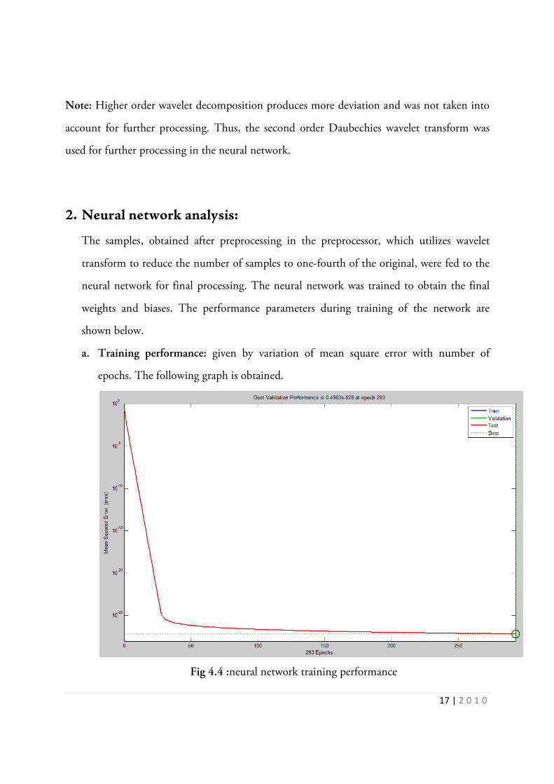
a. Training performance: given by variation of mean square error with number of

epochs. The following graph is obtained.

Fig 4.4 :neural network training performance

18 | 2 0 1 0

It can be observed that the mean square error decreases rapidly till epoch 30 and after

that decreases slowly. A total number of 293 epochs are shown in the in the above

figure. The rapid decrease in the mean square error can be attributed to the use of the

Levenberg-Marquardt algorithm for training of the neural network.

b. Other performance parameters and training state: the following training state

parameters are also obtained during the Neural Network analysis.

Fig 4.5: training state parameters during the training of the network

Note: the weights obtained from the above network are utilized for implementation in

SIMULINK model for real-time implementation.

Note: the accuracy during the training of the network was found to be 99.5%. (Only 1

out of the 200 samples tested returned a negative result). The recognition accuracy can be

increased by training the above neural network with a very large number of samples.

19 | 2 0 1 0

SIMULINK MODEL IMPLEMENTATION

The offline analysis was followed by the implementation of the results so obtained

in a SIMULINK model for simulation of a real-time implementation of the model. The

different parts of the model are described below.

Basically the system structure is same as described in the first chapter. However

the final SIMULINK structure looks like the figure given below. The additional blocks

are due to the different input and output compatibility of the blocks in SIMULINK. For

example, the DWT block takes in a frame based input of frame size of two elements and

the input blocks outputs a frame size of one. Therefore, a buffer block is needed to

convert the frame size from one to two.

Fig : SIMULINK diagram for the whole structure

The individual blocks and their usage are described below.

(i) Input block: This block holds the input values of the signal, which is passed on to

the preprocessing blocks for wavelet decomposition. The frame size of the signal is

one, which is incompatible with the DWT block, which takes in an input of frame

rate 2. Thus, some other blocks are added to the network in between those blocks.

(ii) Matrix flip block: the function of this block is to flip the matrix input from input

block to form a column matrix. This makes the input format of the buffer

compatible with the input block.

(iii) Data type conversion: converts the data format for compatibility.

(iv) Buffer: buffer adjusts the frame rate so that the frame rate is same as that required

by the DWT block.

20 | 2 0 1 0

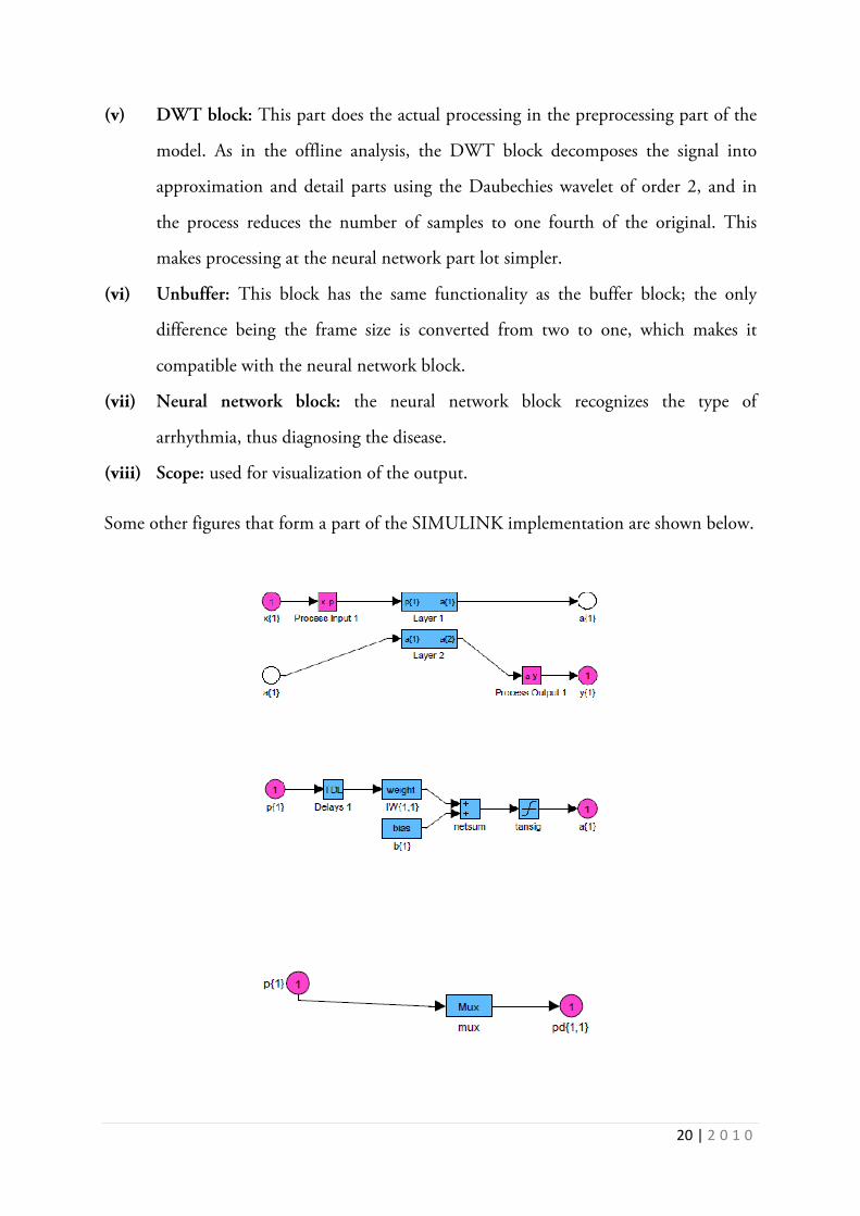
(v) DWT block: This part does the actual processing in the preprocessing part of the

model. As in the offline analysis, the DWT block decomposes the signal into

approximation and detail parts using the Daubechies wavelet of order 2, and in

the process reduces the number of samples to one fourth of the original. This

makes processing at the neural network part lot simpler.

(vi) Unbuffer: This block has the same functionality as the buffer block; the only

difference being the frame size is converted from two to one, which makes it

compatible with the neural network block.

(vii) Neural network block: the neural network block recognizes the type of

arrhythmia, thus diagnosing the disease.

(viii) Scope: used for visualization of the output.

Some other figures that form a part of the SIMULINK implementation are shown below.

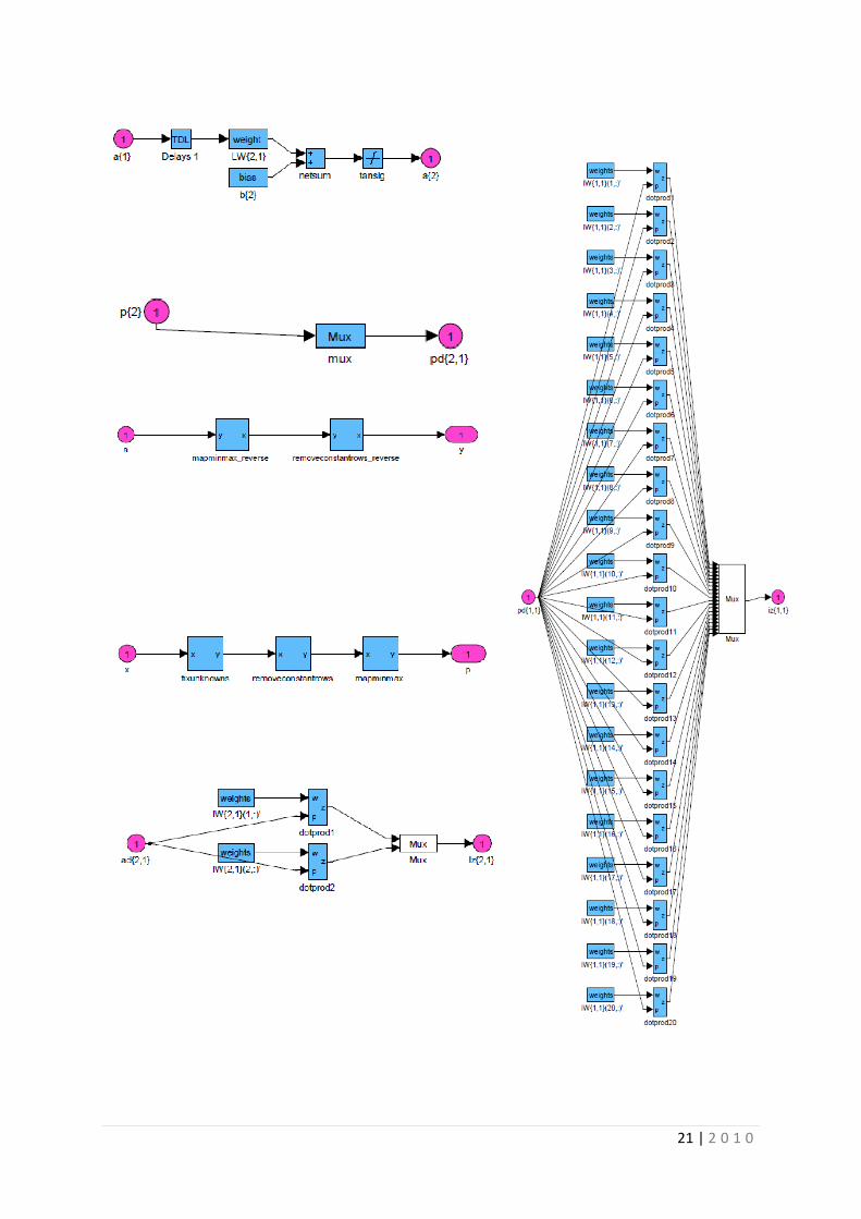
21 | 2 0 1 0

22 |2010

Simulink results

The results of simulation are shown below. The simulation is done with the help of a

synthesized input signal. The topmost figure is the source signal and the subsequent are

normal sinus atrial fibrillation and supraventricular arrhythmia respectively.

fig 5.2 SIMULINK simulation result

������ � � � �

�

CONCLUSION AND FUTURE WORK

Realtime ECG processing holds a great potential for development. Automated

arrhythmia detection could not only help in early detection of diseases but also in

reducing the workload of the medical data analyst. The aim of Discrete Wavelet

Transform is to reduce the number of samples and eventually reducing the complexity of

the neural network and the computation time of the neural network.

However, modern technology has made intensive processing highly feasible and

economical. Computing platforms such as FPGA, PLD, DSP and microprocessors can be

used for interfacing the model with the actual Holter Device.

Of all devices mentioned above FPGA is the most promising because of its speed

and flexibility. FPGA platforms provide great support for many types of interfacing

standards and are hence recommended for implementation in a realtime scenario.

Microprocessors, though not as fast as the FPGA platform also holds great promise as

they are relatively in expensive and are easier to program.

The algorithms given here utilise data from 19 subjects. Training the model with a

large number of test data would greatly enhance the accuracy and hence the reliability of

the system.

24 | 2 0 1 0

REFERENCES

[1]. Acharya, R., Bhat, P. S., Iyengar, S. S., Roo, A., & Dua, S. “Classification of

heart rate data using artificial neural network and Fuzzy equivalence relation”, The

Journal of the Pattern Recognition Society, 2002.

[2]. Osowski, S., & Linh, T. H., “ECG beat recognition using fuzzy hybrid neural

network”, IEEE Transaction on Biomedical Engineering, 2001.

[3]. Ceylan, R. & Ozbay, Y. “Comparison of FCM, PCA and WT techniques for

classification ECG arrhythmias using artificial neural network,” Expert Systems with

Applications, 2007.

[4]. Neural Networks, A Systematic Introduction by Raul Rojas

[5]. A Combinatorial Model for ECG Interpretation, Costas S. Iliopoulos, Spiros

Michalakopoulos.

[6]. ECG Signal Analysis Using Wavelet Transforms, C. Saritha, V. Sukanya, Y.

Narasimha Murthy, 2008.

[7]. Ecg peak detection using wavelet transform, M. A. Khayer and M. A. Haque,

2004

[8]. Ecg signals processing using wavelets, Gordan Cornelia, Reiz Romulus.

[9]. The Wikipedia.