Embed Size (px)
Citation preview

There are many situations in algebraic topology where the relationship between
certain homotopy, homology, or cohomology groups is expressed perfectly by an exact
sequence. In other cases, however, the relationship may be more complicated and
a more powerful algebraic tool is needed. In a wide variety of situations spectral
sequences provide such a tool. For example, instead of considering just a pair (X,A)and the associated long exact sequences of homology and cohomology groups, one
could consider an arbitrary increasing sequence of subspaces X0 ⊂ X1 ⊂ ··· ⊂ Xwith X = ⋃
i Xi , and then there are associated homology and cohomology spectral
sequences. Similarly, the Mayer-Vietoris sequence for a decomposition X = A ∪ Bgeneralizes to a spectral sequence associated to a cover of X by any number of sets.
With this great increase in generality comes, not surprisingly, a corresponding
increase in complexity. This can be a serious obstacle to understanding spectral se-
quences on first exposure. But once the initial hurdle of ‘believing in’ spectral se-
quences is surmounted, one cannot help but be amazed at their power.
1.1 The Homology Spectral SequenceOne can think of a spectral sequence as a book consisting of a sequence of pages,
each of which is a two-dimensional array of abelian groups. On each page there are
maps between the groups, and these maps form chain complexes. The homology
groups of these chain complexes are precisely the groups which appear on the next
page. For example, in the Serre spectral sequence for homology the first few pages
have the form shown in the figure below, where each dot represents a group.
1 2 3
Only the first quadrant of each page is shown because outside the first quadrant all
the groups are zero. The maps forming chain complexes on each page are known as

2 Chapter 1 The Serre Spectral Sequence
differentials. On the first page they go one unit to the left, on the second page two
units to the left and one unit up, on the third page three units to the left and two units
up, and in general on the r th page they go r units to the left and r − 1 units up.
If one focuses on the group at the (p, q) lattice point in each page, for fixed pand q , then as one keeps turning to successive pages, the differentials entering and
leaving this (p, q) group will eventually be zero since they will either come from or go
to groups outside the first quadrant. Hence, passing to the next page by computing
homology at the (p, q) spot with respect to these differentials will not change the
(p, q) group. Since each (p, q) group eventually stabilizes in this way, there is a
well-defined limiting page for the spectral sequence. It is traditional to denote the
(p, q) group of the r th page as Erp,q , and the limiting groups are denoted E∞p,q . In the
diagram above there are already a few stable groups on pages 2 and 3, the dots in the
lower left corner not joined by arrows to other dots. On each successive page there
will be more such dots.
The Serre spectral sequence is defined for fibrations F→X→B and relates the
homology of F , X , and B , under an added technical hypothesis which is satisfied
if B is simply-connected, for example. As it happens, the first page of the spectral
sequence can be ignored, like the preface of many books, and the important action
begins with the second page. The entries E2p,q on the second page are given in terms
of the homology of F and B by the strange-looking formula E2p,q = Hp
(B;Hq(F ;G)
)where G is a given coefficient group. (One can begin to feel comfortable with spectral
sequences when this formula no longer looks bizarre.) After the E2 page the spectral
sequence runs its mysterious course and eventually stabilizes to the E∞ page, and this
is closely related to the homology of the total space X of the fibration. For example,
if the coefficient group G is a field then Hn(X;G) is the direct sum⊕p E
∞p,n−p of the
terms along the nth diagonal of the E∞ page. For a nonfield G such as Z one can
only say this is true ‘modulo extensions’ — the fact that in a short exact sequence
of abelian groups 0→A→B→C→0 the group B need not be the direct sum of the
subgroup A and the quotient group C , as it would be for vector spaces.
As an example, suppose Hi(F ;Z) and Hi(B;Z) are zero for odd i and free abelian
for even i . The entries E2p,q of the E2 page are then zero unless p and q are even.
Since the differentials in this page go up one row, they must all be zero, so the E3
page is the same as the E2 page. The differentials in the E3 page go three units to
the left so they must all be zero, and the E4 page equals the E3 page. The same
reasoning applies to all subsequent pages, as all differentials go an odd number of
units upward or leftward, so in fact we have E2 = E∞ . Since all the groups E∞p,n−pare free abelian there can be no extension problems, and we deduce that Hn(X;Z)is the direct sum
⊕pHp
(B;Hn−p(F ;Z)
). By the universal coefficient theorem this is
isomorphic to⊕pHp(B;Z)⊗Hn−p(F ;Z) , the same answer we would get if X were
simply the product F×B , by the Kunneth formula.

Homology Section 1.1 3
The main difficulty with computing H∗(X;G) from H∗(F ;G) and H∗(B;G) in
general is that the various differentials can be nonzero, and in fact often are. There
is no general technique for computing these differentials, unfortunately. One either
has to make a deep study of the fibration in question and really understand the in-
ner workings of the spectral sequence, or one has to hope for lucky accidents that
yield purely formal calculation of differentials. The situation is somewhat better for
the cohomology version of the Serre spectral sequence. This is quite similar to the
homology spectral sequence except that differentials go in the opposite direction, as
one might guess, but there is in addition a cup product structure which in favorable
cases allows many more differentials to be computed purely formally.
It is also possible sometimes to run the Serre spectral sequence backwards, if
one already knows H∗(X;G) and wants to deduce the structure of H∗(B;G) from
H∗(F ;Z) or vice versa. In this reverse mode one does detective work to deduce the
structure of each page of the spectral sequence from the structure of the following
page. It is rather amazing that this method works as often as it does, and we will see
several instances of this.
Exact Couples
Let us begin by considering a fairly general situation, which we will later specialize
to obtain the Serre spectral sequence. Suppose one has a space X expressed as the
union of a sequence of subspaces ··· ⊂ Xp ⊂ Xp+1 ⊂ ··· . Such a sequence is called
a filtration of X . In practice it is usually the case that Xp = ∅ for p < 0, but
we do not need this hypothesis yet. For example, X could be a CW complex with
Xp its p skeleton, or more generally the Xp ’s could be any increasing sequence of
subcomplexes whose union is X . Given a filtration of a space X , the various long exact
sequences of homology groups for the pairs (Xp,Xp−1) , with some fixed coefficient
group G understood, can be arranged neatly into the following large diagram:
-n 1 p p 1+ −−−→−−−→ XXH ( )n 1 p+ XH ( ) ,
-p p 1XX ,
-p 2-p 1 −−−→ −→−→ −−−→ X )n XH ( - -p 1n XH () -p 2n 1 XH ( ),
n 1 pp 1+
−−−→−−→
−−→−−−→
−−−→−−→
−−→−−−→
−−−→−−→
−−→−−−→ −−−→−−→ XXH ( )n 1 p 1+ + +XH ( ) ,
pp 1 XX + ,
p −−−→ −→−→ −−−→ )n XH ( -nH () -p 1n 1 XH ( )
n 1 p 2+ −−→−−→ XXH ( )n 1 p 2+ + + p 1+ p 1+XH ( ) , −−−→ −→−→ −−−→ )n XH ( -nH () pn 1 XH ( )
The long exact sequences form ‘staircases,’ with each step consisting of two arrows to
the right and one arrow down. Note that each group Hn(Xp) or Hn(Xp,Xp−1) appears
exactly once in the diagram, with absolute and relative groups in alternating columns.
We will call such a diagram of interlocking exact sequences a staircase diagram.

4 Chapter 1 The Serre Spectral Sequence
We may write the preceding staircase diagram more concisely as
the triangle at the right, where A is the direct sum of all the absolute−−−−−→−−−−−→−−−−−→
A
E
i
jk
A
groups Hn(Xp) and E is the direct sum of all the relative groups
Hn(Xp,Xp−1) . The maps i , j , and k are the maps forming the long exact sequences
in the staircase diagram, so the triangle is exact at each of its three corners. Such a
triangle is called an exact couple, where the word ‘couple’ is chosen because there are
only two groups involved, A and E .
For the exact couple arising from the filtration with Xp the p skeleton of a CW
complex X , the map d = jk is just the cellular boundary map. This suggests that
d may be a good thing to study for a general exact couple. For a start, we have
d2 = jkjk = 0 since kj = 0, so we can form the homology group Kerd/ Imd . In
fact, something very nice now happens: There is a derived couple
shown in the diagram at the right, where: −−−−−→−−−−−→
−−−−−→A
E
i
jk
A′′
′′
′
′— E′ = Kerd/ Imd , the homology of E with respect to d .
— A′ = i(A) ⊂ A .
— i′ = i|A′ .— j′(ia) = [ja] ∈ E′ . This is well-defined: ja ∈ Kerd since dja = jkja = 0; and
if ia1 = ia2 then a1 − a2 ∈ Ker i = Imk so ja1 − ja2 ∈ Im jk = Imd .
— k′[e] = ke , which lies in A′ = Im i = Ker j since e ∈ Kerd implies jke = de = 0.
Further, k′ is well-defined since [e] = 0 ∈ E′ implies e ∈ Imd ⊂ Im j = Kerk .
Lemma 1.1. The derived couple of an exact couple is exact.
Proof: This is an exercise in diagram chasing, which we present in condensed form.
— j′i′ = 0: a′ ∈ A′ ⇒ a′ = ia⇒ j′i′a′ = j′ia′ = [ja′] = [jia] = 0.
— Ker j′ ⊂ Im i′ : j′a′ = 0, a′ = ia ⇒ [ja] = j′a′ = 0 ⇒ ja ∈ Imd ⇒ ja = jke ⇒a− ke ∈ Ker j = Im i ⇒ a− ke = ib ⇒ i(a− ke) = ia = i2b ⇒ a′ = ia ∈ Im i2 =Im i′ .
— k′j′ = 0: a′ = ia⇒ k′j′a′ = k′[ja] = kja = 0.
— Kerk′ ⊂ Im j′ : k′[e] = 0⇒ ke = 0⇒ e = ja⇒ [e] = [ja] = j′ia = j′a′ .— i′k′ = 0: i′k′[e] = i′ke = ike = 0.
— Ker i′ ⊂ Imk′ : i′(a′) = 0⇒ i(a′) = 0⇒ a′ = ke = k′[e] . tu
The process of forming the derived couple can now be iterated indefinitely. The
maps d = jk are called differentials, and the sequence E, E′, ··· with differentials
d,d′, ··· is called a spectral sequence: a sequence of groups Er and differentials
dr :Er→Er with d2r = 0 and Er+1 = Kerdr/ Imdr . Note that the pair (Er , dr ) de-
termines Er+1 but not dr+1 . To determine dr+1 one needs additional information.
This information is contained in the original exact couple, but often in a way which is
difficult to extract, so in practice one usually seeks other ways to compute the subse-

Homology Section 1.1 5
quent differentials. In the most favorable cases the computation is purely formal, as
we shall see in some examples with the Serre spectral sequence.
Let us look more closely at the earlier staircase diagram. To simplify notation, set
A1n,p = Hn(Xp) and E1
n,p = Hn(Xp,Xp−1) . The diagram then has the following form:
−−−→−−−→n 1 p+A , -p 1 −−−→ −→−→ −−−→nA - -p 2n 1A−−−→−−→
−−→−−−→
−−−→−−→
−−→−−−→
−−−→−−→
−−→−−−→
1n 1 p+E , ,1 1
-p 1nE , ,1 1
−−−→−−−→n 1+ p 1+
p 2+ p 2+ +
p 1+A , −−−→ −→−→ −−−→nA - -p 1n 1A1n 1 p p+E , ,1 1
nE , ,1 1
−−−→−−−→n 1+A , p 1 +p 1−−−→ −−→−→ −−−→nA - pn 1A1n 1+E , ,1 1
nE , ,1 1
A staircase diagram of this form determines an exact couple, so let us see how the
diagram changes when we pass to the derived couple. Each group A1n,p is replaced by
a subgroup A2n,p , the image of the term A1
n,p−1 directly above A1n,p under the vertical
map i1 . The differentials d1 = j1k1 go two units to the right, and we replace the term
E1n,p by the term E2
n,p = Kerd1/ Imd1 where the two d1 ’s in this formula are the d1 ’s
entering and leaving E1n,p . The terms in the derived couple form a planar diagram
which has almost the same shape as the preceding diagram:
−−−→n 1 p+A , -p 1 −−−→−−→ nA - -p 2n 1A−−−→−−→
−−→−−−→
−−−→−−→
−−→−−−→
−−−→−−→
−−→−−−→
2n 1 p+E , ,2 2
-p 1nE , ,2 2
−−−→n 1+ p 1+
p 2+ p 2+ +
p 1+A , −−−→−−→ nA - -p 1n 1A2n 1 p p+E , ,2 2
nE , ,2 2
−−−→−−−→
−−−→
−−−→−−−→
−−−→
−−−→
−−−→−−−→
−−−→−−−→−−−→
n 1+A , p 1 +p 1−−−→−−→ nA - pn 1A2n 1+E , ,2 2
nE , ,2 2
The maps j2 now go diagonally upward because of the formula j2(i1a) = [j1a] ,from the definition of the map j in the derived couple. The maps i2 and k2 still go
vertically and horizontally, as is evident from their definition, i2 being a restriction
of i1 and k2 being induced by k1 .
Now we repeat the process of forming the derived couple, producing the following
diagram in which the maps j3 now go two units upward and one unit to the right.
−−−→n 1 p+A , -p 1 −−−→−−→ nA - -p 2n 1A−−−→−−→
−−→−−−→
−−−→−−→
−−→−−−→
−−−→−−→
−−→−−−→
3n 1 p+E , ,3 3
-p 1nE , ,3 3
−−−→n 1+ p 1+
p 2+ p 2+ +
p 1+A , −−−→−−→ nA - -p 1n 1A3n 1 p p+E , ,3 3
nE , ,3 3
−−−→−−−−−−−→−−−
−−−−→
−−−−−−−→ −−−
−−−−→−−−
−−−−→
−−−−−−−→−−−
−−−−→
−−−−−−−→
n 1+A , p 1 +p 1−−−→−−→ nA - pn 1A3n 1+E , ,3 3
nE , ,3 3

6 Chapter 1 The Serre Spectral Sequence
This pattern of changes from each exact couple to the next obviously continues in-
definitely. Each Arn,p is replaced by a subgroup Ar+1n,p , and each Ern,p is replaced by a
subquotient Er+1n,p — a quotient of a subgroup, or equivalently, a subgroup of a quo-
tient. Since a subquotient of a subquotient is a subquotient, we can also regard all the
Ern,p ’s as subquotients of E1n,p , just as all the Arn,p ’s are subgroups of A1
n,p .
We now make some simplifying assumptions about the algebraic staircase dia-
gram consisting of the groups A1n,p . These conditions will be satisfied in the applica-
tion to the Serre spectral sequence. Here is the first condition:
(i) All but finitely many of the maps in each A column are isomorphisms.. By exact-
ness this is equivalent to saying that only finitely many terms in each E column
are nonzero.
Thus at the top of each A column the groups An,p have a common value A1n,−∞ and
at the bottom of the A column they have the common value A1n,∞ . For example, in
the case that A1n,p = Hn(Xp) , if we assume that Xp = ∅ for p < 0 and the inclusions
XpX induce isomorphisms on Hn for sufficiently large p , then (i) is satisfied, with
A1n,−∞ = Hn(∅) = 0 and A1
n,∞ = Hn(X) .Since the differential dr goes upward r −1 rows, condition (i) implies that all the
differentials dr into and out of a given E column must be zero for sufficiently large
r . In particular, this says that for fixed n and p , the terms Ern,p are independent of
r for sufficiently large r . These stable values are denoted E∞n,p . Our immediate goal
is to relate these groups E∞n,p to the groups A1n,∞ or A1
n,−∞ under one of the following
two additional hypotheses:
(ii) A1n,−∞ = 0 for all n .
(iii) A1n,∞ = 0 for all n .
If we look in the r th derived couple we see the term Ern,p embedded in an exact
sequence
Ern+1,p+r−1kr-----→Arn,p+r−2
i-----→Arn,p+r−1jr-----→Ern,p
kr-----→Arn−1,p−1i-----→Arn−1,p
jr-----→Ern−1,p−r+1
Fixing n and p and letting r be large, the first and last E terms in this sequence are
zero by condition (i). If we assume condition (ii) holds, the last two A terms in the
sequence are zero by the definition of Ar . So in this case the exact sequence expresses
Ern,p as the quotient Arn,p+r−1/i(Arn,p+r−2) , or in other words, ir−1(A1
n,p)/ir (A1
n,p−1) ,a quotient of subgroups of A1
n,p+r−1 = A1n,∞ . Thus E∞n,p is isomorphic to the quotient
Fpn/Fp−1n where Fpn denotes the image of the map A1
n,p→A1n,∞ . Summarizing, we have
shown the first of the following two statements:
Proposition 1.2. Under the conditions (i) and (ii) the stable group E∞n,p is isomor-
phic to the quotient Fpn/Fp−1n for the filtration ··· ⊂ Fp−1
n ⊂ Fpn ⊂ ··· of A1n,∞ by
the subgroups Fpn = Im(A1n,p→A1
n,∞). Assuming (i) and (iii), E∞n,p is isomorphic to
Fn−1p /Fn−1
p−1 for the filtration ··· ⊂ Fn−1p−1 ⊂ Fn−1
p ⊂ ··· of A1n−1,−∞ by the subgroups
Fn−1p = Ker
(A1n−1,−∞→A1
n−1,p).

Homology Section 1.1 7
Proof: For the second statement, condition (iii) says that the first two A terms in the
previous displayed exact sequence are zero, so the exact sequence represents Ern,p as
the kernel of the map Arn−1,p−1→Arn−1,p . For large r all elements of these two groups
come from A1n−1,−∞ under iterates of the vertical maps i , so Ern,p is isomorphic to
the quotient of the subgroup of A1n−1,−∞ mapping to zero in A1
n−1,p by the subgroup
mapping to zero in A1n−1,p−1 . tu
In the topological application where we start with the staircase diagram of ho-
mology groups associated to a filtration of a space X , we have Hn(X) filtered by the
groups Fpn = Im(Hn(Xp)→Hn(X)) . The group
⊕p F
pn/F
p−1n is called the associated
graded group of the filtered group Hn(X) . The proposition then says that this graded
group is isomorphic to⊕p E
∞n,p . More concisely, one says simply that the spectral se-
quence converges to H∗(X) . We remind the reader that these are homology groups
with coefficients in an arbitrary abelian group G which we have omitted from the
notation, for simplicity.
The analogous situation for cohomology is covered by the condition (iii). Here we
again have a filtration of X by subspaces Xp with Xp = ∅ for p < 0, and we assume
that the inclusion Xp X induces an isomorphism on Hn for p sufficiently large
with respect to n . The associated staircase diagram has the form
n 1+−−−→−−−→ XH ( )n 1pXH ( )-
-
-- -
--
-
p p 1XX , X
-p p 1XX ,
p 1
-
p 1 −−−→ −→−→ −−−→ X )n XH ( p 2n XH () p 2
n 1 XH ( ),
n 1+
−−−→−−→
−−→−−−→
−−−→−−→
−−→−−−→
−−−→−−→
−−→−−−→ −−−→−−→H ( )n 1
p 1XH ( )
pp 1 X+ ,
pp 1 X+
+
++
+++ +
,p −−−→ −→−→ −−−→ )n XH (n H () p 1n 1 XH ( )
n 1p 1
+−−→−−→ XXH ( )n 1p 2 p 2 p 1
+
XH ( ) , −−−→ −→−→ −−−→ )n XH (n H () pn 1 XH ( )
We have isomorphisms at the top of each A column and zeros at the bottom, so the
conditions (i) and (iii) are satisfied. Hence we have a spectral sequence converging
to H∗(X) . If we modify the earlier notation and now write An,p1 = Hn(Xp) and
En,p1 = Hn(Xp,Xp−1) , then after translating from the old notation to the new we
find that Hn(X) is filtered by the subgroups Fnp = Ker(Hn(X)→Hn(Xp−1)
)with
En,p∞ ≈ Fnp /Fnp+1 .

8 Chapter 1 The Serre Spectral Sequence
The Main Theorem
Now we specialize to the situation of a fibration π :X→B with B a path-connected
CW complex and we filter X by the subspaces Xp = π−1(Bp) , Bp being the p skeleton
of B . Since (B, Bp) is p connected, the homotopy lifting property implies that (X,Xp)is also p connected, so the inclusion XpX induces an isomorphism on Hn(−;G) if
n < p . This, together with the fact that Xp = ∅ for p < 0, is enough to guarantee that
the spectral sequence for homology with coefficients in G associated to this filtration
of X converges to H∗(X;G) , as we observed a couple pages back.
The E1 term consists of the groups E1n,p = Hn(Xp,Xp−1;G) . These are nonzero
only for n ≥ p since (Bp, Bp−1) is (p − 1) connected and hence so is (Xp,Xp−1) . In
view of this we make a change of notation by setting n = p + q , and then we use the
parameters p and q instead of n and p . Thus our spectral sequence now has its E1
page consisting of the terms E1p,q = Hp+q(Xp,Xp−1;G) , and these are nonzero only
when p ≥ 0 and q ≥ 0. In the old notation we had differentials dr :Ern,p→Ern−1,p−r ,
so in the new notation we have dr :Erp,q→Erp−r ,q+r−1 .
What makes this spectral sequence so useful is the fact that there is a very nice
formula for the entries on the E2 page in terms of the homology groups of the fiber
and the base spaces. This formula takes its simplest form for fibrations satisfying a
mild additional hypothesis that can be regarded as a sort of orientability condition
on the fibration. To state this, let us recall a basic construction for fibrations. Under
the assumption that B is path-connected, all the fibers Fb = π−1(b) are homotopy
equivalent to a fixed fiber F since each path γ in B lifts to a homotopy equivalence
Lγ :Fγ(0)→Fγ(1) between the fibers over the endpoints of γ , as shown in the proof
of Proposition 4.61 of [AT] . In particular, restricting γ to loops at a basepoint of Bwe obtain homotopy equivalences Lγ :F→F for F the fiber over the basepoint. Using
properties of the association γ, Lγ shown in the proof of 4.61 of [AT] it follows
that when we take induced homomorphisms on homology, the association γ, Lγ∗defines an action of π1(B) on H∗(F ;G) . The condition we are interested in is that
this action is trivial, meaning that Lγ∗ is the identity for all loops γ .
Theorem 1.3. Let F→X→B be a fibration with B path-connected. If π1(B) acts
trivially on H∗(F ;G) , then there is a spectral sequence Erp,q, dr with :
(a) dr :Erp,q→Erp−r ,q+r−1 and Er+1p,q = Kerdr/ Imdr at Erp,q .
(b) stable terms E∞p,n−p isomorphic to the successive quotients Fpn/Fp−1n in a filtration
0 ⊂ F0n ⊂ ··· ⊂ Fnn = Hn(X;G) of Hn(X;G) .
(c) E2p,q ≈ Hp(B;Hq(F ;G)) .
It is instructive to look at the special case that X is the product B×F . The Kunneth
formula and the universal coefficient theorem then combine to give an isomorphism
Hn(X;G) ≈⊕pHp(B;Hn−p(F ;G)) . This is what the spectral sequence yields when all
differentials are zero, which implies that E2 = E∞ , and when all the group extensions

Homology Section 1.1 9
in the filtration of Hn(X;G) are trivial, so that the latter group is the direct sum of the
quotients Fpn/Fp−1n . Nontrivial differentials mean that E∞ is ‘smaller’ than E2 since in
computing homology with respect to a nontrivial differential one passes to proper sub-
groups and quotient groups. Nontrivial extensions can also result in smaller groups.
For example, the middle Z in the short exact sequence 0→Z→Z→Zn→0 is ‘smaller’
than the product of the outer two groups, Z⊕Zn . Thus we may say that H∗(B×F ;G)provides an upper bound on the size of H∗(X;G) , and the farther X is from being a
product, the smaller its homology is.
An extreme case is when X is contractible, as for example in a path space fibrationΩX→PX→X . Let us look at two examples of this type, before getting into the proof
of the theorem.
Example 1.4. Using the fact that S1 is a K(Z,1) , let us compute the homology of
a K(Z,2) without using the fact that CP∞ happens to be a K(Z,2) . We apply the
Serre spectral sequence to the pathspace fibration F→P→B where B is a K(Z,2)and P is the space of paths in B starting at the basepoint, so P is contractible and
the fiber F is the loopspace of B , a K(Z,1) . Since B is simply-connected, the Serre
spectral sequence can be applied for homology with Z coefficients. Using the fact that
Hi(F ;Z) is Z for i = 0,1 and 0 otherwise, only the first two rows of the E2 page can
be nonzero. These have the following form.
0
1
0 1 2 3 4 5 6
H B( )1 H B( )2 H B( )3 H B( )4 H B( )5 H B( )6Z
H B( )1 H B( )2 H B( )3 H B( )4 H B( )5 H B( )6Z −−−−−−−−−−−−→ −−−−−−−−−−−−→ −−−−−−−−−−−−→−−−−−−−−−−−−→−−−−−−−−−−−−→
Since the total space P is contractible, only the Z in the lower left corner survives to
the E∞ page. Since none of the differentials d3, d4, ··· can be nonzero, as they go
upward at least two rows, the E3 page must equal the E∞ page, with just the Z in the
(0,0) position. The key observation is now that in order for the E3 page to have this
form, all the differentials d2 in the E2 page going from the q = 0 row to the q = 1
row must be isomorphisms, except for the one starting at the (0,0) position. This
is because any element in the kernel or cokernel of one of these differentials would
give a nonzero entry in the E3 page. Now we finish the calculation of H∗(B) by an
inductive argument. By what we have just said, the H1(B) entry in the lower row is
isomorphic to the implicit 0 just to the left of the Z in the upper row. Next, the H2(B)in the lower row is isomorphic to the Z in the upper row. And then for each i > 2,
the Hi(B) in the lower row is isomorphic to the Hi−2(B) in the upper row. Thus we
obtain the result that Hi(K(Z,2);Z) is Z for i even and 0 for i odd.
Example 1.5. In similar fashion we can compute the homology of ΩSn using the
pathspace fibration ΩSn→P→Sn . The case n = 1 is trivial since ΩS1 has con-

10 Chapter 1 The Serre Spectral Sequence
tractible components, as one sees by lifting loops to the universal cover of S1 . So we
assume n ≥ 2, which means the base space Sn of the fibration is simply-connected
so we have a Serre spectral sequence for homol-
ogy. Its E2 page is nonzero only in the p = 0
and p = n columns, which each consist of the
homology groups of the fiber ΩSn . As in the
0
n - 1
3n - 3
2n - 2
0 n
Z
H ΩS( )n -1n
H ΩS( )2n - 2n
H ΩS( )3n - 3n H ΩS( )3n - 3
n
H ΩS( )2n - 2n
H ΩS( )n - 1n
Z
−−−−−−−−−→−−−−−−−−−→−−−−−−−−−→
preceding example, the E∞ page must be triv-
ial, with just a Z in the (0,0) position. The only
differential which can be nonzero is dn , so we
have E2 = E3 = ··· = En and En+1 = ··· = E∞ .
The dn differentials from the p = n column to
the p = 0 column must be isomorphisms, apart from the one going to the Z in the
(0,0) position. It follows by induction that Hi(ΩSn;Z) is Z for i a multiple of n− 1
and 0 for all other i .This calculation could also be made without spectral sequences, using Theo-
rem 4J.1 of [AT] which says that ΩSn is homotopy equivalent to the James reduced
product JSn−1 , whose cohomology (hence also homology) is computed in §3.2 of [AT].
Now we give an example with slightly more complicated behavior of the differen-
tials and also nontrivial extensions in the filtration of H∗(X) .
Example 1.6. To each short exact sequence of groups 1→A→B→C→1 there is
associated a fibration K(A,1)→K(B,1)→K(C,1) that can be constructed by realizing
the homomorphism B→C by a map K(B,1)→K(C,1) and then converting this into
a fibration. From the associated long exact sequence of homotopy groups one sees
that the fiber is a K(A,1) . For this fibration the action of the fundamental group
of the base on the homology of the fiber will generally be nontrivial, but it will be
trivial for the case we wish to consider now, the fibration associated to the sequence
0→Z2→Z4→Z2→0, using homology with Z coefficients, since RP∞ is a K(Z2,1)and Hn(RP∞;Z) is at most Z2 for n > 0, while for n = 0 the action is trivial since in
general π1(B) acts trivially on H0(F ;G) whenever F is path-connected.
Z2
Z 2
Z 2Z 2Z 2Z 2Z 2Z 2Z 2Z2Z −−−−−−−−−−−−−−−−−−−−−−−−−−−−−−−−−−−−−−−−−−−−−−−−−→
−−−−−−−−−−−−−−−−−−−−−−−−−−−−−−−−−−−−−−−−−−−−−−−−−→
−−−−−−−−−−−−−−−−−−−−−−−−−−−−−−−−−−−−−−−−−−−−−−−−−→
−−−−−−−−−−−−−−−−−−−−−−−−−−−−−−−−−−−−−−−−−−−−−−−−−→
−−−−−−−−−−−−−−−−−−−−−−−−−−−−−−−−−−−−−−−−−−−−−−−−−→
−−−−−−−−−−−−−−−−−−−−−−−−−−−−−−−−−−−−−−−−−−−−−−−−−→
−−−−−−−−−−−−−−−−−→ −−−−−−−−−−−−−−−−−→ −−−−−−−−−−−−−−−−−→ −−−−−−−−−−−−−−−−−→0
0
1 3 5
0 Z 2 0 Z 2 0 Z 2 Z 20
2 4
21
0 0 00 0 0 0 02Z 2Z 2Z 2Z 2Z 2Z2Z0 0 00 0 02Z 2Z 2Z 2Z2Z0 0 002Z
2Z
2Z2Z0 0
43
6789
5
6 7 8 9
A portion of the E2 page of the spectral sequence is shown at the left.
If we were dealing with the product fibration with total space
K(Z2,1)×K(Z2,1) , all the differentials would be zero and
the extensions would be trivial, as noted earlier, but
for the fibration with total space K(Z4,1) we
will show that the only nontrivial differ-
entials are those indicated by ar-
rows, hence the only terms
that survive to the E∞
page are the circled
groups. To see this

Homology Section 1.1 11
we look along each diagonal line p + q = n . The terms along this diagonal are the
successive quotients for some filtration of Hn(K(Z4,1);Z) , which is Z4 for n odd,
and 0 for even n > 0. This means that by the time we get to E∞ all the Z2 ’s in the
unshaded diagonals in the diagram must have become 0, and along each shaded di-
agonal all but two of the Z2 ’s must have become 0. To see that the differentials are as
drawn we start with the n = 1 diagonal. There is no chance of nonzero differentials
here so both the Z2 ’s in this diagonal survive to E∞ . In the n = 2 diagonal the Z2
must disappear, and this can only happen if it is hit by the differential originating at
the Z2 in the (3,0) position. Thus both these Z2 ’s disappear in E3 . This leaves two
Z2 ’s in the n = 3 diagonal, which must survive to E∞ , so there can be no nonzero
differentials originating in the n = 4 diagonal. The two Z2 ’s in the n = 4 diagonal
must then be hit by differentials from the n = 5 diagonal, and the only possibility is
the two differentials indicated. This leaves just two Z2 ’s in the n = 5 diagonal, so
these must survive to E∞ . The pattern now continues indefinitely.
Proof of Theorem 1.3: We will first give the proof when B is a CW complex and then at
the end give the easy reduction to this special case. When B is a CW complex we have
already proved statements (a) and (b). To prove (c) we will construct an isomorphism
of chain complexes
-p q pd
p 1+ p q 1+−−−−−−−−−−−−−−−−−−−−−−−−−→−−−−−−−−−−−−−→ XX GH ( ), ; G;-p 2 −−−−−−−−−−−−−→X )-- p 1XH ( ,−−−→ −−−→. . . . . .
-p
1
p p 1p 1−−−−−−−−−−−−−−−−−−→−−−→ BB GH ( q FH ( )), ; ; ;
-p 2 −−−→B--p 1BH ( ,. . . . . .Z ⊗ Gq FH ( )) ;Z ⊗∂ 11⊗
≈ ≈Ψ ΨThe lower row is the cellular chain complex for B with coefficients in Hq(F ;G) , so (c)
will follow.
The isomorphisms Ψ will be constructed via the following commutative diagram:
F GHq ( ) FHq ( )-B BHpp 1p( ),; G;;
-X X GHp q p 1p( ), ;G; +−−→ −−→αα α
αα
∼ ∼∼ -D SHp qp 1p
p
( ),+ −−−−−→∗Φ⊕
α⊕⊕
⊗Ψε
≈≈ ≈
≈ Z
Let Φα :Dpα→Bp be a characteristic map for the p cell epα of B , so the restriction
of Φα to the boundary sphere Sp−1α is an attaching map for epα and the restriction
of Φα to Dpα − Sp−1α is a homeomorphism onto epα . Let Dpα = Φ∗α(Xp) , the pullback
fibration over Dpα , and let Sp−1α be the part of Dpα over Sp−1
α . We then have a mapΦ :∐α (D
pα, S
p−1α ) -→ (Xp,Xp−1) . Since Bp−1 is a deformation retract of a neighbor-
hood N in Bp , the homotopy lifting property implies that the neighborhood π−1(N)of Xp−1 in Xp deformation retracts onto Xp−1 , where the latter deformation retrac-
tion is in the weak sense that points in the subspace need not be fixed during the
deformation, but this is still sufficient to conclude that the inclusion Xp−1π−1(N)is a homotopy equivalence. Using the excision property of homology, this implies that
12 Chapter 1 The Serre Spectral Sequence
Φ induces the isomorphism Φ∗ in the diagram. The isomorphism in the lower row of
the diagram comes from the splitting of Hp(Bp, Bp−1;Z) as the direct sum of Z ’s, one
for each p cell of B .
To construct the left-hand vertical isomorphism in the diagram, consider a fibra-
tion Dp→Dp . We can partition the boundary sphere Sp−1 of Dp into hemispheres
Dp−1± intersecting in an equatorial Sp−2 . Iterating this decomposition, and letting
tildes denote the subspaces of Dp lying over these subspaces of Dp , we look at the
following diagram, with coefficients in G implicit:∼ ∼ -D SHp q
p 1 ∼ -Sp 2∼ -Dp 1p
( ), ,+
∼ --DHp q 1p 1∼ -
- Sp 1( ),+
−−−−−→−−−−−→ −−−−−→
−−−−−→ −−−−−→-Hp q 1( )+ −−−−−→ −−−−−→∗
+ +
∂ i
ε . . .
. . .≈≈
∼ ∼D SHq 1
1 0 ∼D0
( ),+
∼-DHq0∼
S 0( ),
−−−−−→−−−−−→
−−−−−→Hq ( )
∗
+
∂ i
ε
≈≈
The first boundary map is an isomorphism from the long exact sequence for the triple
(Dp, Sp−1, Dp−1− ) using the fact that Dp deformation retracts to Dp−1
− , lifting the
corresponding deformation retraction of Dp onto Dp−1− . The other boundary maps
are isomorphisms for the same reason. The isomorphisms i∗ come from excision.
Combining these isomorphisms we obtain the isomorphisms ε . Taking Dp to be
Dpα , the isomorphism εpα in the earlier diagram is then obtained by composing the
isomorphisms ε with isomorphisms Hq(D0α;G) ≈ Hq(Fα;G) ≈ Hq(F ;G) where Fα =Φα(D0
α) , the first isomorphism being induced by Φα and the second being given by
the hypothesis of trivial action, which guarantees that the isomorphisms Lγ∗ depend
only on the endpoints of γ .
Having identified E1p,q with Hp(B
p, Bp−1;Z)⊗Hq(F ;G) , we next identify the dif-
ferential d1 with ∂ ⊗11. Recall that the cellular boundary map ∂ is determined by
the degrees of the maps Sp−1α →Sp−1
β obtained by composing the attaching map ϕαfor the cell epα with the quotient maps Bp−1→Bp−1/Bp−2→Sp−1
β where the latter map
collapses all (p−1) cells except ep−1β to a point, and the resulting sphere is identified
with Sp−1β using the characteristic map for ep−1
β .
On the summand Hq(F ;G) of Hp+q(Xp,Xp−1;G) corresponding to the cell epαthe differential d1 is the composition through the lower left corner in the following
commutative diagram:
-X XHp q p 1p( ),+
−−→ −−→ −−→
−−−−−→ - XHp q 1( )+ - -X XHp q 1 p 2-p 1-p 1 ( ),+−−−−−→α
α
α∼∼ ∼ ∼∼
∂
-D SHp qp 1
α∼ -Sp 1 α
∼ -Sp 1 α∼ -Dp 1p
( ),+ −−−−−→ -Hp q 1( )+ -Hp q 1( ),+−−−−−→∂
∗ α∗ϕ α∗ϕΦBy commutativity of the left-hand square this composition through the lower left
corner is equivalent to the composition using the middle vertical map. To compute
this composition we are free to deform ϕα by homotopy and lift this to a homotopy
of ϕα . In particular we can homotope ϕα so that it sends a hemisphere Dp−1α to
Xp−2 , and then the right-hand vertical map in the diagram is defined. To determine

Homology Section 1.1 13
this map we will use another commutative diagram whose left-hand map is equivalent
to the right-hand map in the previous diagram:
−−→−−→
−−−−−→- -X XHp q 1 p 2- -p 1( ),+
i i ii iα∼∼ ∼-Dp 1
α∼ -S p 2 −−−−−→-Hp q 1( ),+
∼ -Dp 1∼ -S p 2-Hp q 1( ),+
∼ -Dp 1∼ -S p 2-Hp q 1( ),+
α∗ϕ
−−→
−−−−−−−−−−−−−−−−−−→- -X X eHp q 1 p 1-p 1-
-
p 1( ),+
α∼
∼
-Dp 1α∼ -Dp 1 ∼ -Dp 1 −−−−−→-Hp q 1( ( )),+
α∗ϕ
β β β
int ∪ ≈
≈
⊕
To obtain the middle vertical map in this diagram we perform another homotopy of
ϕα so that it restricts to homeomorphisms from the interiors of a finite collection of
disjoint disks Dp−1i in Dp−1
α onto ep−1β and sends the rest of Dp−1
α to the complement
of ep−1β in Bp−1 . (This can be done using Lemma 4.10 of [AT], for example.) Via the iso-
morphisms Ψ we can identify some of the groups in the diagram with Hq(F ;G) . The
map across the top of the diagram then becomes the diagonal map, x, (x, ··· , x) .It therefore suffices to show that the right-hand vertical map, when restricted to the
Hq(F ;G) summand corresponding to Di , is 11 or −11 according to whether the degree
of ϕα on Di is 1 or −1.
The situation we have is a pair of fibrations Dk→Dk and Dk→Dk and a map ϕbetween them lifting a homeomorphism ϕ :Dk→Dk . If the degree of ϕ is 1, we may
homotope it, as a map of pairs (Dk, Sk−1)→(Dk, Sk−1) , to be the identity map and lift
this to a homotopy of ϕ . Then the evident naturality of εk gives the desired result.
When the degree of ϕ is −1 we may assume it is a reflection, namely the reflection
interchanging D0+ and D0
− and taking every other Di± to itself. Then naturality gives
a reduction to the case k = 1 with ϕ a reflection of D1 . In this case we can again use
naturality to restate what we want in terms of reparametrizing D1 by the reflection
interchanging its two ends. The long exact sequence for the pair (D1, S0) breaks up
into short exact sequences
0 -→Hq+1(D1, S0;G) ∂-----→Hq(S
0;G) i∗-----→Hq(D1;G) -→0
The inclusions D0± D1 are homotopy equivalences, inducing isomorphisms on ho-
mology, so we can view Hq(S0;G) as the direct sum of two copies of the same group.
The kernel of i∗ consists of pairs (x,−x) in this direct sum, so switching the roles
of D0+ and D0
− in the definition of ε has the effect of changing the sign of ε . This
finishes the proof when B is a CW complex.
To obtain the spectral sequence when B is not a CW complex we let B′→B be a
CW approximation to B , with X′→B′ the pullback of the given fibration X→B . There
is a map between the long exact sequences of homotopy groups for these two fibra-
tions, with isomorphisms between homotopy groups of the fibers and bases, hence
also isomorphisms for the total spaces. By the Hurewicz theorem and the universal
coefficient theorem the induced maps on homology are also isomorphisms. The ac-
tion of π1(B′) on H∗(F ;G) is the pullback of the action of π1(B) , hence is trivial
by assumption. So the spectral sequence for X′→B′ gives a spectral sequence for
X→B . tu
14 Chapter 1 The Serre Spectral Sequence
Serre Classes
We turn now to an important theoretical application of the Serre spectral se-
quence. Let C be one of the following classes of abelian groups:
(a) FG , finitely generated abelian groups.
(b) TP , torsion abelian groups whose elements have orders divisible only by primes
from a fixed set P of primes.
(c) FP , the finite groups in TP .
In particular, P could be all primes, and then TP would be all torsion abelian groups
and FP all finite abelian groups.
For each of the classes C we have:
Theorem 1.7. If X is simply-connected, then πn(X) ∈ C for all n iff Hn(X;Z) ∈ C
for all n > 0 . This holds also if X is path-connected and abelian, that is, the action
of π1(X) on πn(X) is trivial for all n ≥ 1 .
The coefficient group for homology will always be Z throughout this section, and
we will write Hn(X) for Hn(X;Z) .
The theorem says in particular that a simply-connected space has finitely gener-
ated homotopy groups iff it has finitely generated homology groups. For example, this
says that πi(Sn) is finitely generated for all i and n . Prior to this theorem of Serre
it was only known that these homotopy groups were countable, as a consequence of
simplicial approximation.
For nonabelian spaces the theorem can easily fail. As a simple example, S1 ∨S2 has π2 nonfinitely generated although Hn is finitely generated for all n . And
in §4.A of [AT] there are more complicated examples of K(π,1) ’s with π finitely
generated but Hn not finitely generated for some n . For the class of finite groups,
RP2n provides an example of a space with finite reduced homology groups but at
least one infinite homotopy group, namely π2n . There are no such examples in the
opposite direction, as finite homotopy groups always implies finite reduced homology
groups. The argument for this is outlined in the exercises.
The theorem can be deduced as a corollary of a version of the Hurewicz theorem
that gives conditions for the Hurewicz homomorphism h :πn(X)→Hn(X) to be an
isomorphism modulo the class C , meaning that the kernel and cokernel of h belong
to C .
Theorem 1.8. If a path-connected abelian space X has πi(X) ∈ C for i < n then
the Hurewicz homomorphism h :πn(X)→Hn(X) is an isomorphism modC .
For the proof we need two lemmas.

Homology Section 1.1 15
Lemma 1.9. Let F→X→B be a fibration of path-connected spaces, with π1(B) act-
ing trivially on H∗(F) . Then if two of F , X , and B have Hn ∈ C for all n > 0 , so
does the third.
Proof: The only facts we shall use about the classes C are the following two properties,
which are easy to verify for each class in turn:
(1) For a short exact sequence of abelian groups 0→A→B→C→0, the group B is
in C iff A and C are both in C .
(2) If A and B are in C , then A⊗B and Tor(A, B) are in C .
There are three cases in the proof of the lemma:
Case 1: Hn(F),Hn(B) ∈ C for all n > 0. In the Serre spectral sequence we then have
E2p,q = Hp(B;Hq(F)) ≈ Hp(B)⊗Hq(F)
⊕Tor(Hp−1(B),Hq(F)) ∈ C for (p, q) ≠ (0,0) .
Suppose by induction on r that Erp,q ∈ C for (p, q) ≠ (0,0) . Then the subgroups
Kerdr and Imdr are in C , hence their quotient Er+1p,q is also in C . Thus E∞p,q ∈ C
for (p, q) ≠ (0,0) . The groups E∞p,n−p are the successive quotients in a filtration
0 ⊂ F0n ⊂ ··· ⊂ Fnn = Hn(X) , so it follows by induction on p that the subgroups Fpn
are in C for n > 0, and in particular Hn(X) ∈ C .
Case 2: Hn(F),Hn(X) ∈ C for all n > 0. Since Hn(X) ∈ C , the subgroups filtering
Hn(X) lie in C , hence also their quotients E∞p,n−p . Assume inductively that Hp(B) ∈ C
for 0 < p < k . As in Case 1 this implies E2p,q ∈ C for p < k , (p, q) ≠ (0,0) , and hence
also Erp,q ∈ C for the same values of p and q .
Since Er+1k,0 = Kerdr ⊂ Erk,0 , we have a short exact sequence
0 -→Er+1k,0 -→Erk,0
dr-----→ Imdr -→0
with Imdr ⊂ Erk−r ,r−1 , hence Imdr ∈ C since Erk−r ,r−1 ∈ C by the preceding para-
graph. The short exact sequence then says that Er+1k,0 ∈ C iff Erk,0 ∈ C . By downward
induction on r we conclude that E2k,0 = Hk(B) ∈ C .
Case 3: Hn(B),Hn(X) ∈ C for all n > 0. This case is quite similar to Case 2 and will
not be used in the proof of the theorem, so we omit the details. tu
Lemma 1.10. If π ∈ C then Hk(K(π,n)) ∈ C for all k,n > 0 .
Proof: Using the path fibration K(π,n−1)→P→K(π,n) and the previous lemma it
suffices to do the case n = 1. For the classes FG and FP the group π is a product of
cyclic groups in C , and K(G1,1)×K(G2,1) is a K(G1×G2,1) , so by either the Kunneth
formula or the previous lemma applied to product fibrations, which certainly satisfy
the hypothesis of trivial action, it suffices to do the case that π is cyclic. If π = Z we
are in the case C = FG , and S1 is a K(Z,1) , so obviously Hk(S1) ∈ C . If π = Zm we
know that Hk(K(Zm,1)) is Zm for odd k and 0 for even k > 0, since we can choose
an infinite-dimensional lens space for K(Zm,1) . So Hk(K(Zm,1)) ∈ C for k > 0.

16 Chapter 1 The Serre Spectral Sequence
For the class TP we use the construction in §1.B in [AT] of a K(π,1) CW complex
Bπ with the property that for any subgroup G ⊂ π , BG is a subcomplex of Bπ . An
element x ∈ Hk(Bπ) with k > 0 is represented by a singular chain∑i niσi with
compact image contained in some finite subcomplex of Bπ . This finite subcomplex
can involve only finitely many elements of π , hence is contained in a subcomplex BGfor some finitely generated subgroup G ⊂ π . Since G ∈ FP , by the first part of the
proof we know that the element of Hk(BG) represented by∑i niσi has finite order
divisible only by primes in P , so the same is true for its image x ∈ Hk(Bπ) . tu
Proof of 1.7 and 1.8: We assume first that X is simply-connected. Consider a Post-
nikov tower for X ,
··· -→Xn -→Xn−1 -→··· -→X2 = K(π2(X),2)
where Xn→Xn−1 is a fibration with fiber Fn = K(πn(X),n) . If πi(X) ∈ C for all i ,then by induction on n the two lemmas imply that Hi(Xn) ∈ C for i > 0. Up to ho-
motopy equivalence, we can build Xn from X by attaching cells of dimension greater
than n+ 1, so Hi(X) ≈ Hi(Xn) for n ≥ i , and therefore Hi(X) ∈ C for all i > 0.
The Hurewicz maps πn(X)→Hn(X) and πn(Xn)→Hn(Xn) are equivalent, and
we will deal with the latter via the fibration Fn→Xn→Xn−1 . The associated spectral
sequence has nothing between the 0th and nth rows, so the first interesting differen-
tial is dn+1 :Hn+1(Xn−1)→Hn(Fn) . This fits into a five-term exact sequence
X −−−−−→-Hn 1
n0
n 1( )+ X -H 0
0 0
n n 1( )F −−−−−−−−−−−−−−−−→−−−−−→
−−−−−→−−−−−→
−−−−−→−−−−−→ −−−−−→H
E
n n( ) XHn n( )
,∞
n 0E ,∞
=
coming from the filtration of Hn(Xn) . If we assume that πi(X) ∈ C for i < n then
πi(Xn−1) ∈ C for all i , so by the preceding paragraph the first and fourth terms
of the exact sequence above are in C , and hence the map Hn(Fn)→Hn(Xn) is an
isomorphism mod C . This map is just the one induced by the inclusion map Fn→Xn .
F −−−−−−−−−−−−−−−−→Hn n( ) XHn n( )
Fh
−−−−−−−−−−−−−−−−→n n( ) Xn n( )π π−−→
h
−−→≈≈In the commutative square shown at the right the upper
map is an isomorphism from the long exact sequence of
the fibration. The left-hand map is an isomorphism by the
usual Hurewicz theorem since F is (n− 1) connected. We
have just seen that the lower map is an isomorphism modC , so it follows that this is
also true for the right-hand map. This finishes the proof for X simply-connected.
In case X is not simply-connected but just abelian we can apply the same argu-
ment using a Postnikov tower of principal fibrations Fn→Xn→Xn−1 . As observed
in §4.3 of [AT], these fibrations have trivial action of π1(Xn−1) on πn(Fn) , which
means that the homotopy equivalences Fn→Fn inducing this action are homotopic
to the identity since Fn is an Eilenberg-MacLane space. Hence the induced action on

Homology Section 1.1 17
Hi(Fn) is also trivial, and the Serre spectral sequence can be applied just as in the
simply-connected case. tu
Supplements
Fiber Bundles
The Serre spectral sequence is valid for fiber bundles as well as for fibrations.
Given a fiber bundle p :E→B , the map p can be converted into a fibration by the usual
pathspace construction. The map from the fiber bundle to the fibration then induces
isomorphisms on homotopy groups of the base and total spaces, hence also for the
fibers by the five-lemma, so the map induces isomorphisms on homology groups as
well, by the relative Hurewicz theorem. For fiber bundles as well as fibrations there
is a notion of the fundamental group of the base acting on the homology of the fiber,
and one can check that this agrees with the action we have defined for fibrations.
Alternatively one could adapt the proof of the main theorem to fiber bundles,
using a few basic facts about fiber bundles such as the fact that a fiber bundle with
base a disk is a product bundle.
Relative Versions
There is a relative version of the spectral sequence. Given a fibration F→X π-----→Band a subspace B′ ⊂ B , let X′ = π−1(B′) , so we have also a restricted fibration
F→X′→B′ . In this situation there is a spectral sequence converging to H∗(X,X′;G)
with E2p,q = Hp
(B, B′;Hq(F ;G)
), assuming once again that π1(B) acts trivially on
H∗(F ;G) . To obtain this generalization we first assume that (B, B′) is a CW pair,
and we modify the original staircase diagram by replacing the pairs (Xp,Xp−1) by the
triples (Xp ∪X′, Xp−1∪X′, X′) . The A columns of the diagram consist of the groups
Hn(Xp∪X′, X′;G) and the E columns consist of the groups Hn(Xp∪X′, Xp−1∪X′;G) .Convergence of the spectral sequence to H∗(X,X
′;G) follows just as before since
Hn(Xp∪X′, X′;G) = Hn(X,X′;G) for sufficiently large p . The identification of the E2
terms also proceeds just as before, the only change being that one ignores everything
in X′ and B′ . To treat the case that (B, B′) is not a CW pair, we may take a CW pair
approximating (B, B′) , as in §4.1 of [AT].
Local Coefficients
There is a version of the spectral sequence for the case that the fundamental
group of the base space does not act trivially on the homology of the fiber. The only
change in the statement of the theorem is to regard Hp(B;Hq(F ;G)
)as homology
with local coefficients. The latter concept is explained in §3.H of [AT], and the reader
familiar with this material should have no difficulty is making the necessary small
modifications in the proof to cover this case.

18 Chapter 1 The Serre Spectral Sequence
General Homology Theories
The construction of the Serre spectral sequence works equally well for a general
homology theory, provided one restricts the base space B to be a finite-dimensional
CW complex. There is certainly a staircase diagram with ordinary homology replaced
by any homology theory h∗ , and the finiteness condition on B says that the filtration
of X is finite, so the convergence condition (ii) holds trivially. The proof of the theorem
shows that E2p,q = Hp(B;hq(F)) . A general homology theory need not have hq = 0 for
q < 0, so the spectral sequence can occupy the fourth quadrant as well as the first.
However, the hypothesis that B is finite-dimensional guarantees that only finitely
many columns are nonzero, so all differentials in Er are zero when r is sufficiently
large. For infinite-dimensional B the convergence of the spectral sequence can be a
more delicate question.
As a special case, if the fibration is simply the identity map X→X we obtain a
spectral sequence converging to h∗(X) with E2p,q = Hp(X;hq(point)) . This is known
as the Atiyah-Hirzebruch spectral sequence, as is its cohomology analog.
Naturality
The spectral sequence satisfies predictable naturality properties. Suppose we
are given two fibrations and a map between them, a commutative
diagram as at the right. Suppose also that the hypotheses of the
−−→ −−→ −−→−−→ −−→F X B−−→ −−→
F X B′ ′ ′∼f f
main theorem are satisfied for both fibrations. Then the naturality
properties are:
(a) There are induced maps f r∗ :Erp,q→E′rp,q commuting with differentials, with f r+1∗
the map on homology induced by f r∗ .
(b) The map f∗ :H∗(X;G)→H∗(X′;G) preserves filtrations, inducing a map on suc-
cessive quotient groups which is the map f∞∗ .
(c) Under the isomorphisms E2p,q ≈ Hp
(B;Hq(F ;G)
)and E′2p,q ≈ Hp
(B′;Hq(F
′;G))
the map f 2∗ corresponds to the map induced by the maps B→B′ and F→F ′ .
To prove these it suffices to treat the case that B and B′ are CW complexes, by natu-
rality properties of CW approximations. The map f can then be deformed to a cellular
map, with a corresponding lifted deformation of f . Then f induces a map of stair-
case diagrams, and statements (a) and (b) are obvious. For (c) we must reexamine the
proof of the main theorem to see that the isomorphisms Ψ commute with the maps
induced by f and f . It suffices to look at what is happening over cells epα of B and
epβ of B′ . We may assume f has been deformed so that fΦα sends the interiors of
disjoint subdisks Dpi of Dpα homeomorphically onto epβ and the rest of Dpα to the
complement of epβ . Then we have a diagram similar to one in the proof of the main
theorem:

Homology Section 1.1 19
−−→−−→
−−−−−→-X XHp q p 1p( ),+
i i ii iα∼∼∼D
pα∼ -S p 1 −−−−−→H
fp q ( ),+
∼Dp ∼ -S p 1Hp q ( ),+
∼Dp ∼ -S p 1Hp q ( ),+
α∗∗
−−→
−−−−−−−−−−−−−−−−−−→-X X eHp q p 1p-
-
p( ),+
α∼
∼
Dpα∼Dp ∼
Dp −−−−−→Hp q ( ( )),+
β β β
int ∪ ≈
≈
⊕′ ′ ′ ′Φ ∼∼f α∗∗Φ
This gives a reduction to the easy situation that f is a homeomorphism Dp→Dp ,
which one can take to be either the identity or a reflection. (Further details are left to
the reader.)
In particular, for the case of the identity map, naturality says that the spectral
sequence, from the E2 page onward, does not depend in any way on the CW structure
of the base space B , if B is a CW complex, or on the choice of a CW approximation to
B in the general case.
By considering the map from the given fibration p :X→B to the identity fibration
B→B we can use naturality to describe the induced map p∗ :H∗(X;G)→H∗(B;G)in terms of the spectral sequence. In the commutative
square at the right, where the two E∞n,0 ’s are for the two −−→ −−→−−−−−→
GXHn
E Xn 0
( )
( ) B( )
;
,
GBHn( );
∞
−−→
En 0,∞
p∗
=fibrations, the right-hand vertical map is the identity, so
the square gives a factorization of p∗ as the composi-
tion of the natural surjection Hn(X;G)→E∞n,0 coming from the filtration in the first
fibration, followed by the lower horizontal map. The latter map is the composition
E∞n,0(X) E2n,0(X)→E2
n,0(B) = E∞n,0(B) whose second map will be an isomorphism if
the fiber F of the fibration X→B is path-connected. In this case we have factored
p∗ as the composition Hn(X;G)→E∞n,0(X)→Hn(B;G) of a surjection followed by
an injection. Such a factorization must be equivalent to the canonical factorization
Hn(X;G)→ Imp∗Hn(B;G) .
Z2Z −−−−−−−−−−−−−−−−−−−−−−−−−−−−−−−−−
−−−−−−−−−−−−−−−−−−−−−−−−−−−−−−−−−−−−−−−−−−−−−−−−−−−−−−−−−−
−−−−−−−−−−−−−−−−−−−−−−−−−−−−−−−−−−−−−−−−−−−−−−−−−−−−−−−−−−−−−
−−−−−−−−−−−−−−−−−−−−−−−−−−−−−−−−−−−−−−−−−−→
−−−−−−−−−−−−−−−−−−−−−−−−−−−−−−−−−−−−−−−−−−−−−−−−−−−−−−−−−−−−−−−−
−−−−−−−−−−−−−−−−−−−−−−−−−−−−−−−−−−−−−−−−−−−−−−−−−−−−−−−−−−−−−−
−−−−−−−−−−−−−−→
−−−−−−−−−−−−−−−−−−−−−−−−−−−−−−−−−−−−−−−−−−−−−−−−−−−−−−−−−−−−−−−−
−−−−−−−−−−−−−−−−−−−−−−−−−−−−−−−−−−−−−−−−−−−−−−−−−−−−−−−−−−−−−−−
−−−−−−−−−−−−−→
−−−−−−−−−−−−−−−−−−−−−−−−−−−−−−−−−−−−−−−−−−−−−−−−−−−−−−−−−−−−−−−−−−−−−−−−
−−−−−−−−−−−−−−−→−−−−−−−−−−−−−−−−−−−−−−−−−−−−−−−−−−−−
−−−−−−−−−−−−−−−−−−−−−−−−−−−−−−−−−−−−−−−−−−−−−−−−−−−→
−−−−−−−−−−−−−−−−−−−−−−−−−−−−−−−−−−−−−−−−−−−−−−−−−−−−−−−−−−−−−−−−−−−−−−−
−−−−−−−−−−−−−−−−→
−−−−−−−−−−−−−−−−−→ −−−−−−−−−−−−−−−−−→ −−−−−−−−−−−−−−−−−→ −−−−−−−−−−−−−−−−−→0
0
1 3 52 4
21
0 000
2Z0 0
0
2Z0 0
0
000
00
000
000 0
00
00
2Z
2Z0
Z2Z02Z02Z
Z2Z02Z
Z2Z
Z2Z
02Z
02Z
02Z
00
43
6789
5
6 7 8 9
Example 1.11. Let us illustrate this by considering the fibration p :K(Z,2)→K(Z,2)inducing multiplication by 2 on π2 , so the fiber is a K(Z2,1) . Differentials originating
above the 0th row must have source or target 0 so must be trivial. By contrast, every
differential from a Z in the 0th row to a Z2 in an upper row must
be nontrivial, for otherwise a leftmost surviving Z2 would con-
tribute a Z2 subgroup to H∗(K(Z,2);Z) . Thus E∞2n,0 is the
subgroup of E22n,0 of index 2n , and hence the image
of p∗ :H2n(K(Z,2);Z)→H2n(K(Z,2);Z) is the
subgroup of index 2n . The more stan-
dard proof of this fact would use
the cup product structure in
H∗(CP∞;Z) , but here
we have a proof us-
ing only homology.

20 Chapter 1 The Serre Spectral Sequence
Spectral Sequence Comparison
We can use these naturality properties of the Serre spectral sequence to prove
two of the three cases of the following result.
Proposition 1.12. Suppose we have a map of fibrations as in the discussion of natu-
rality above, and both fibrations satisfy the hypothesis of trivial action for the Serre
spectral sequence. Then if two of the three maps F→F ′ , B→B′ , and X→X′ induce
isomorphisms on H∗(−;R) with R a principal ideal domain, so does the third.
This can be viewed as a sort of five-lemma for spectral sequences. It can be
formulated as a purely algebraic statement about spectral sequences, known as the
Spectral Sequence Comparison Theorem; see [MacLane] for a statement and proof of
the algebraic result.
Proof: First we do the case of isomorphisms in fiber and base. Since R is a PID,
it follows from the universal coefficient theorem for homology of chain complexes
over R that the induced maps Hp(B;Hq(F ;R))→Hp(B′;Hq(F ′;R)) are isomorphisms.
Thus the map f2 between E2 terms is an isomorphism. Since f2 induces f3 , which
in turn induces f4 , etc., the maps fr are all isomorphisms, and in particular f∞ is
an isomorphism. The map Hn(X;R)→Hn(X′;R) preserves filtrations and induces
the isomorphisms f∞ between successive quotients in the filtrations, so it follows by
induction and the five-lemma that it restricts to an isomorphism on each term Fpn in
the filtration of Hn(X;R) , and in particular on Hn(X;R) itself.
Now consider the case of an isomorphism on fiber and total space. Let f :B→B′be the map of base spaces. The pullback fibration then fits into a commutative diagram
as at the right. By the first case, the map E→f∗(E′) induces an −−→ −−→ −−→
−−→ −−→ −−→
−−→
−−→−→ −→F
E
B B B
f
f
E
F ′
′ E′
′
F ′===
===
( )∗isomorphism on homology, so it suffices to deal with the second
and third fibrations. We can reduce to the case that f is an
inclusion BB′ by interpolating between the second and third
fibrations the pullback of the third fibration over the mapping
cylinder of f . A deformation retraction of this mapping cylinder onto B′ lifts to a
homotopy equivalence of the total spaces.
Now we apply the relative Serre spectral sequence, with E2 = H∗(B′, B;H∗(F ;R)
)converging to H∗(E
′, E;R) . If Hi(B′, B;R) = 0 for i < n but Hn(B
′, B;R) is nonzero,
then the E2 array will be zero to the left of the p = n column, forcing the nonzero
term E2n,0 = Hn
(B′, B;H0(F ;R)
)to survive to E∞ , making Hn(E
′, E;R) nonzero.
We will not prove the third case, as it is not needed in this book. tu
Transgression
The Serre spectral sequence can be regarded as the more complicated analog for
homology of the long exact sequence of homotopy groups associated to a fibration

Homology Section 1.1 21
F→X→B , and in this light it is natural to ask whether there is anything in homol-
ogy like the boundary homomorphisms πn(B)→πn−1(F) in the long exact sequence
of homotopy groups. To approach this ques-
tion, the diagram at the right is the first thing
to look at. The map j∗ is an isomorphism, as-
−−−−−→ −−−−−→−−−−−→
FXH Hn( ) F( ),
bBHn( ),BHn( )
-n 1∂
p∗j∗
suming n > 0, so if the map p∗ were also an
isomorphism we would have a boundary map Hn(B)→Hn−1(F) just as for homotopy
groups. However, p∗ is not generally an isomorphism, even in the case of simple
products X = F×B . Thus if we try to define a boundary map by sending x ∈ Hn(B)to ∂p−1
∗ (j∗x) , this only gives a homomorphism from a subgroup of Hn(B) , namely
(j∗)−1(Imp∗) , to a quotient group of Hn−1(F) , namely Hn−1(F)/∂(Kerp∗) . This
homomorphism goes by the high-sounding name of the transgression. Elements of
Hn(B) that lie in the domain of the transgression are said to be transgressive.
The transgression may seem like an awkward sort of object, but it has a nice
description in terms of the Serre spectral sequence:
Proposition 1.13. The transgression is exactly the differential dn :Enn,0→En0,n−1 .
In particular, the domain of the transgression is the subgroup of E2n,0 = Hn(B)
on which the differentials d2, ··· , dn−1 vanish, and the target is the quotient group
of E20,n−1 = Hn−1(F) obtained by factoring out the images of the same collection
of differentials d2, ··· , dn−1 . Sometimes the transgression is simply defined as the
differential in the proposition. We have seen several examples where this differential
played a particularly significant role in the Serre spectral sequence, so the proposition
gives it a topological interpretation.
Proof: The first step is to identify Enn,0 with Imp∗ :Hn(X, F)→Hn(B, b) . For this
it is helpful to look also at the relative Serre spectral sequence for the fibration
(X, F)→(B, b) , which we distinguish from the original spectral sequence by using
the notation Er . We also now use p∗ for the map Hn(X, F)→Hn(B, b) . The two
spectral sequences have the same E2 page except that the p = 0 column of E2 is
replaced by zeros in E2since H0(B, b) = 0, as B is path-connected by assumption.
This implies that the map E3p,q→E3
p,q is injective for p > 0 and an isomorphism for
p ≥ 3. One can then see inductively that the map Erp,q→Erp,q is injective for p > 0
and an isomorphism for p ≥ r . In particular, when we reach the En page we still
have Enn,0 = Enn,0 . The differential dn originating at this term is automatically zero
in En , so Enn,0 = E∞n,0 . The latter group is Imp∗ :Hn(X, F)→Hn(B, b) by the relative
form of the remarks on naturality earlier in this section. Thus Enn,0 = Imp∗ .
For the remainder of the proof we use the following diagram:

22 Chapter 1 The Serre Spectral Sequence
−−−−−→−−−−−→
−−−−−→−−−−−→
−−−−−→−−−−−→
−−−−−→−−−−−→
−−−−−→
−−−−−→−−−−−→ FXHn( )
( )
XHn( ) ,
,
FH ( )-n 1
-n 1
−−−−−→ XH ( )-n 1i∗j
d
∗
p q∗ p∗
∂
−−−−−→∂ ∂
−−−−−→−−−−−→−−−−−→ −−−−−→ −−−−−→nEn 0,En 0 ,nn E0 -n 1,E 0
0
00
0 0∞∞
,En 0∞
-
pKer ∗-
pIm ∗- -pIm ∗
−−−−−→−−−−−→0
0
pKer ∗-
= =
=
The two longer rows are obviously exact, as are the first two columns. In the next
column q is the natural quotient map so it is surjective. Verifying exactness of this
column then amounts to showing that Kerq = ∂(Kerp∗) . Once we show this and
that the diagram commutes, then the proposition will follow immediately from the
subdiagram consisting of the two vertical short exact sequences, since this subdiagram
identifies the differential dn with the transgression Imp∗→Hn−1(F)/∂(Kerp∗) .The only part of the diagram where commutativily may not be immediately evi-
dent is the middle square containing dn . To see that this square commutes we extract
a few relevant terms from the staircase diagram that leads to the original spectral se-
quence, namely the terms E1n,0 and E1
0,n−1 . These fit into a diagram−−−−−→ −−−−−→
−−−−−→ −−−−−→FXHn( ),
−−−−−→FXHn n( ), XHn n X
E
( ), ,
FH ( )-n 1 -n 1 -n 1
-n 1
d
q
p∗
∂−−−−−−−−−−−−−−−−−−−−−−
−−−−−−−−−−−→1En 0 ,
nEn 0
,10 E ,
n0
n-
=
=
We may assume B is a CW complex with b as its single 0 cell, so X0 = F in the
filtration of X , hence E10,n−1 = Hn−1(F) . The vertical map on the left is surjective
since the pair (X,Xn) is n connected. The map dn is obtained by restricting the
boundary map to cycles whose boundary lies in F , then taking this boundary. Such
cycles represent the subgroup Enn,0 , and the resulting map is in general only well-
defined in the quotient group En0,n−1 of Hn−1(F) . However, if we start with an element
in Hn(Xn, F) in the upper-left corner of the diagram and represent it by a cycle, its
boundary is actually well-defined in Hn−1(F) rather than in the quotient group. Thus
the outer square in this diagram commutes. The upper triangle commutes by the
earlier description of p∗ in terms of the relative spectral sequence. Hence the lower
triangle commutes as well, which is the commutativity we are looking for.
Once one knows the first diagram commutes, then the fact that Kerq = ∂(Kerp∗)follows from exactness elsewhere in the diagram by the standard diagram-chasing
argument. tu
Homology Section 1.1 23
Exercises
1. Compute the homology of the homotopy fiber of a map Sk→Sk of degree n , for
k,n > 1.
2. Compute the Serre spectral sequence for homology with Z coefficients for the
fibration K(Z2,1)→K(Z8,1)→K(Z4,1) . [See Example 1.6.]
3. For a fibration K(A,1)→K(B,1)→K(C,1) associated to a short exact sequence
of groups 1→A→B→C→1 show that the associated action of π1K(C,1) = C on
H∗(K(A,1);G) is trivial if A , regarded as a subgroup of B , lies in the center of B .
4. Show that countable abelian groups form a Serre class.

24 Chapter 1 The Serre Spectral Sequence
1.2 CohomologyThere is a completely analogous Serre spectral sequence in cohomology:
Theorem 1.14. For a fibration F→X→B with B path-connected and π1(B) acting
trivially on H∗(F ;G) , there is a spectral sequence Ep,qr , dr , with :
(a) dr :Ep,qr →Ep+r ,q−r+1r and Ep,qr+1 = Kerdr/ Imdr at Ep,qr .
(b) stable terms Ep,n−p∞ isomorphic to the successive quotients Fnp /Fnp+1 in a filtration
0 ⊂ Fnn ⊂ ··· ⊂ Fn0 = Hn(X;G) of Hn(X;G) .(c) Ep,q2 ≈ Hp(B;Hq(F ;G)) .
Proof: Translating the earlier derivation for homology to cohomology is straightfor-
ward, for the most part. We use the same filtration of X , so there is a cohomology
spectral sequence satisfying (a) and (b) by our earlier general arguments. To identify
the E2 terms we want an isomorphism of chain complexes
-p q
pd
p 1+ p q 1+ +
++
+−−−−−−−−−−−−−−−−−−−−−−−−−→−−−−−−−−−−−−−→ XX GH ( ), ; G;p −−−−−−−−−−−−−→X )p 1XH ( ,
−−−→ −−−→. . . . . .
-p
1
p p 1p 1−−−−−−−−−−−−−−−−−−→−−−→ BB GH ( q FH ( )), ,; ; ;
p −−−→Bp 1BHHom ((Hom( , ,. . . . . .Z Gq FH ( ))) ) ;Z∂≈ ≈Ψ Ψ∗
The isomorphisms Ψ come from diagrams
F GHq ( ) FH q( ))-B BHHom pp 1p(( ), ,; G;;
-X X GHp qp 1p( ), ;G; +
−−→ −−→αα α
αα
∼ ∼∼ -D SHp q p 1p
p
( ),+ −−−−−→∗Φ
α
Ψε≈
≈ ≈≈ ZΠ
Π∏
The construction of the isomorphisms εpα goes just as before, with arrows reversed
for cohomology.
The identification of d1 with the cellular coboundary map also follows the earlier
scheme exactly. At the end of the argument where signs have to be checked, we now
have the split exact sequence
0 -→Hq(D1;G) i∗-----→Hq(S0;G) δ-----→Hq+1(D1, S0;G) -→0
The middle group is the direct sum of two copies of the same group, correspond-
ing to the two points of S0 , and the exact sequence represents Hq+1(D1, S0;G) as
the quotient of this direct sum by the subgroup of elements (x,x) . Each of the two
summands of Hq(S0;G) maps isomorphically onto the quotient, but the two isomor-
phisms differ by a sign since (x,0) is identified with (0,−x) in the quotient.
There is just one additional comment about d1 that needs to be made. For coho-
mology, the direct sums occurring in homology are replaced by direct products, and
homomorphisms whose domain is a direct product may not be uniquely determined
by their values on the individual factors. If we view d1 as a map∏αH
p+q(Dpα, Sp−1α ;G) ---------→∏
βHp+q+1(Dp+1
β , Spβ ;G)

Cohomology Section 1.2 25
then d1 is determined by its compositions with the projections πβ onto the factors
of the target group. Each such composition πβd1 is finitely supported in the sense
that there is a splitting of the domain as the direct sum of two parts, one consisting
of the finitely many factors corresponding to p cells in the boundary of ep+1β , and the
other consisting of the remaining factors, and the composition πβd1 is nonzero only
on the first summand, the finite product. It is obvious that finitely supported maps
like this are determined by their restrictions to factors. tu
Multiplicative Structure
The Serre spectral sequence for cohomology becomes much more powerful when
cup products are brought into the picture. For this we need to consider cohomology
with coefficients in a ring R rather than just a group G . What we will show is that
the spectral sequence can be provided with bilinear products Ep,qr ×Es,tr →Ep+s,q+tr for
1 ≤ r ≤ ∞ satisfying the following properties:
(a) Each differential dr is a derivation, satisfying d(xy) = (dx)y + (−1)p+qx(dy)for x ∈ Ep,qr . This implies that the product Ep,qr ×Es,tr →Ep+s,q+tr induces a prod-
uct Ep,qr+1×Es,tr+1→Ep+s,q+tr+1 , and this is the product for Er+1 . The product in E∞is the one induced from the products in Er for finite r .
(b) The product Ep,q2 ×Es,t2 →Ep+s,q+t2 is (−1)qs times the standard cup product
Hp(B;Hq(F ;R)
)×Hs(B;Ht(F ;R))→Hp+s(B;Hq+t(F ;R)
)sending a pair of cocycles (ϕ,ψ) to ϕ`ψ where coefficients are multiplied via
the cup product Hq(F ;R)×Ht(F ;R)→Hq+t(F ;R) .(c) The cup product in H∗(X;R) restricts to maps Fmp ×Fns→Fm+np+s . These induce
quotient maps Fmp /Fmp+1×Fns /Fns+1→Fm+np+s /F
m+np+s+1 that coincide with the prod-
ucts Ep,m−p∞ ×Es,n−s∞ →Ep+s,m+n−p−s∞ .
We shall obtain these products by thinking of cup product as the composition
H∗(X;R)×H∗(X;R) ×------------→H∗(X×X;R) ∆∗------------→H∗(X;R)
of cross product with the map induced by the diagonal map ∆ :X→X×X . The prod-
uct X×X is a fibration over B×B with fiber F×F . Since the spectral sequence is
natural with respect to the maps induced by ∆ it will suffice to deal with cross prod-
ucts rather than cup products. If one wanted, one could just as easily treat a product
X×Y of two different fibrations rather than X×X .
There is a small technical issue having to do with the action of π1 of the base on
the cohomology of the fiber. Does triviality of this action for the fibration F→X→Bimply triviality for the fibration F×F→X×X→B×B ? In most applications, includ-
ing all in this book, B is simply-connected so the question does not arise. There
is also no problem when the cross product H∗(F ;R)×H∗(F ;R)→H∗(F×F ;R) is an

26 Chapter 1 The Serre Spectral Sequence
isomorphism. In the general case one can take cohomology with local coefficients for
the spectral sequence of the product, and then return to ordinary coefficients via the
diagonal map.
Now let us see how the product in the spectral sequence arises. Taking the base
space B to be a CW complex, the product X×X is filtered by the subspaces (X×X)pthat are the preimages of the skeleta (B×B)p . There are canonical splittings
Hk((X×X)`, (X×X)`−1
) ≈ ⊕i+j=`
Hk(Xi×Xj,Xi−1×Xj ∪Xi×Xj−1)
that come from the fact that (Xi×Xj)∩ (Xi′ ×Xj′) = (Xi ∩Xi′)×(Xj ∩Xj′) .Consider first what is happening at the E1 level. The product Ep,q1 ×Es,t1 →Ep+s,q+t1
is the composition in the first column of the following diagram, where the second map
is the inclusion of a direct summand. Here m = p + q and n = s + t .
× ×
× ×
×
X XHm Hnp( ), ×-p 1 X Xs( ), -s 1
+×XHm np(( ,X s )) +×X p( X ) -s 1
+
−−−−−−−−→
−−−−−−−−→
−−−−−−−−−−−−−−−−−−−−−−−→
−−−−−−−−−−−−−−−−−−−−−−−→
−−−−−−−−−−−−−−−−−−−−−−−→−−−−−−−−→ −−−−−−−−→
1++×XHm n
p(( ,X s)) + ×Xp ( X )s 1+ +
×X XHm np ×Xp( , -p 1 XXs ×Xs )-s 1
+ ∪
δ δ
δ
δ
-p 1XH X( Xp,p s )s 1∪1m n++s 1+
+
×X XH ×Xp( ,p 1 X
×X ×X ×X
Xs ×Xs )-s 1∪1m n++ p 1+
+
⊕
×
X XHmp( ), ×-p 1
Hn X Xs( ), -s 1- 1H X Xp( ,p 1 )
( )1m
m+
+
H X Xs( ,s 1 )1n++
⊕
⊕
⊕11 11
The derivation property is equivalent to commutativity of the diagram. To see that
this holds we may take cross product to be the cellular cross product defined for CW
complexes, after replacing the filtration X0 ⊂ X1 ⊂ ··· by a chain of CW approxima-
tions. The derivation property holds for the cellular cross product of cellular chains
and cochains, hence it continues to hold when one passes to cohomology, in any rel-
ative form that makes sense, such as in the diagram.
[An argument is now needed to show that each subsequent differential dr is a
derivation. The argument we orginally had for this was inadequate.]
For (c), we can regard Fmp as the image of the map Hm(X,Xp−1)→Hm(X) , via
the exact sequence of the pair (X,Xp−1) . With a slight shift of indices, the following
commutative diagram then shows that the cross product respects the filtration:
×X XHm Hn
p( ), × X Xs( ), −−−−−−−−→−−−−−−−−→ −−−−−−−−−−−−−−−−−−−−−−−→ ×X XHm np ×X( , XX s×X )+ ∪ −−−−−−−−−−−−−−−−−−−−−−−→ ×X XHm n
p( (,X s×X ))++
×XHm Hn( ) × X( ) −−−−−−−−−−−−−−−−−−−−−−−−−−−−−−−−−−−−−−−−−−−−−−−−−−−−−−−−−−−−−−−−−−−−−−−−−−−−−−−−−−−−−−−−−−−−−−−−−−−−−−−−−−−−−−−−−−−−−−−−−−−−−−−−−−−−−−−−−−−−−−−−−−−−−−−−−−−−−−−−−−−−−−−−−−−−−−−−−−−−−−−−−−−−−−−−−−−−−−−−−−−−−−−−−−−−−−−−−−−−−−−−−−−−−−−−−−−−−−−−−−−−−−−−−−−−−−−−−−−−−−−−−−−−−−−−−−−−−−−−−−−−−−−−−−−−−−−−−−−−−−−−−−−−−−−−−−−−−−−−−−−−−−−−−−−−−−−−−−−−−−−−−−−−−−−−−−−−−−−−−−−−−−−−−−−−−−−−−−−−−−−−−−−−−−−−−−−−−−−−−−−−−−−−−−−−−−−−−−−−−−−−−−−−−−−−−−−−−−−−−−−−−−−−−−−−−−−−−−−−−−−−−−−−−−−−−−−−−−−−−−−−−−−−−−−−−−−−−−−−−−−−−−−−−−−−−−−−−−−−−−−−−−−−−−−−−−−−−−−−−−−−−−−−−−−−−−−−−−−−−−−−−−−−−−−−−−−−−−−−−−−−−−−−−−−−−−−−−−−−−−−−−−−−−−−−−−−−−−−−−−−−−−−−−−−−−−−−−−−−−−−−−−−−−−−−−−−−−−−−−−−−−−−−−−−−−−−−−−−−−−−−−−−−−−−−−−−−−−−−−−−−−−−−−−−−−−−−−−−−−−−−−→ ×XHm n( X )+
Recalling how the staircase diagram leads to the relation between E∞ terms and the
successive quotients of the filtration, the rest of (c) is apparent from naturality of
cross products.

Cohomology Section 1.2 27
In order to prove (b) we will use cross products to give an alternative definition
of the isomorphisms Hp+q(Dp, Sp−1) ≈ Hq(F) for a fibration F→Dp→Dp . Such
a fibration is fiber-homotopy equivalent to a product Dp×F since the base Dp is
contractible. By naturality we then have the com-
mutative diagram at the right. The lower εp is theFHq ( )
∼ ∼ -D SHp q p 1pp( ),+
-D F SHp q p 1p( ),+
−−−−−→−−−−−−−−−−−→ ≈
× F×
ε
pεmap λ,γ×λ for γ a generator of Hp(Dp, Sp−1) ,since εp is essentially a composition of coboundary maps of triples, and δ(γ×λ) =δγ×λ from the corresponding cellular cochain formula δ(a×b) = δa×b ± a×δb ,
where δb = 0 in the present case since b is a cocycle representing λ .
Referring back to the second diagram in the proof of 1.14, we have, for λ ∈Hom
(Hp(B
p, Bp−1;Z),Hq(F ;R))
and µ ∈ Hom(Hs(B
s, Bs−1;Z),Ht(F ;R)), the formu-
las Φ∗Ψ(λ×µ)(epα×esβ) = γα×γβ×λ(epα)×µ(esβ)= (−1)qsγα×λ(epα)×γβ×µ(esβ)= (−1)qsΦ∗Ψ(λ)(epα)×Φ∗Ψ(µ)(esβ)
using the commutativity property of cross products and the fact that γα×γβ can
serve as the γ for epα×esβ . Since the isomorphisms Φ∗ preserve cross products, this
finishes the justification for (b).
Cup product is commutative in the graded sense, so the product in E1 and hence
in Er satisfies ab = (−1)|a||b|ba where |a| = p+q for a ∈ Ep,q1 = Hp+q(Xp,Xp−1;R) .This is compatible with the isomorphisms Ψ :Hp(B;Hq(F ;R))→Ep,q2 since for x ∈Hp(B;Hq(F ;R)) and y ∈ Hs(B;Ht(F ;R)) we have
Ψ(x)Ψ(y) = (−1)qsΨ(xy) = (−1)qs+ps+qtΨ(yx)= (−1)qs+ps+qt+ptΨ(y)Ψ(x)= (−1)(p+q)(s+t)Ψ(y)Ψ(x)
It is also worth pointing out that differentials satisfy the familiar-looking formula
d(xn) = nxn−1dx if |x| is even
since d(x ·xn−1) = dx ·xn−1+xd(xn−1) = xn−1dx+(n−1)x ·xn−2dx by induction,
and using the commutativity relation.
Example 1.15. For a first application of the product structure in the cohomology
spectral sequence we shall use the pathspace fibration K(Z,1)→P→K(Z,2) to show
that H∗(K(Z,2);Z) is the polynomial ring Z[x] with x ∈ H2(K(Z,2);Z) . The base
K(Z,2) of the fibration is simply-connected, so we have a Serre spectral sequence
with Ep,q2 ≈ Hp(K(Z,2);Hq(S1;Z)) . The additive structure of the E2 page can be
determined in much the same way that we did for homology in Example 1.4, or we can
simply quote the result obtained there. In any case, here is what the E2 page looks
like:

28 Chapter 1 The Serre Spectral Sequence
Z1 Zx Zx2
2 4 6
4 6Zx . . .
. . .
Za Zax Zax Zax . . .−−−−−−−−→ −−−−−−−−→ −−−−−−−−→ −−−−−−−−→0
0 0 0 0 0
1 3 5 7
0 0 0 0
2 4
1
6
The symbols a and xi denote generators of the groups E0,12 ≈ Z and Ei,02 ≈ Z . The
generators for the Z ’s in the upper row are a times the generators in the lower row
because the product E0,q2 ×Es,t2 -→ Es,q+t2 is just multiplication of coefficients. The
differentials shown are isomorphisms since all terms except Z1 disappear in E∞ . In
particular, d2a generates Zx2 so we may assume d2a = x2 by changing the sign of
x2 if necessary. By the derivation property of d2 we have d2(ax2i) = (d2a)x2i ±a(d2x2i) = (d2a)x2i = x2x2i since d2x2i = 0. Since d2(ax2i) is a generator of
Zx2i+2 , we may then assume x2x2i = x2i+2 . This relation means that H∗(K(Z,2);Z)is the polynomial ring Z[x] where x = x2 .
Example 1.16. Let us compute the cup product structure in H∗(ΩSn;Z) using the
Serre spectral sequence for the path fibration ΩSn→PSn→Sn . The additive struc-
ture can be deduced just as was done for homology
in Example 1.5. The nonzero differentials are isomor-
phisms, shown in the figure to the right. Replacing some
0
n - 1
3n - 3
2n - 2
0 n
x
Z1
1
Zx
Za 1Za−−−−−−−−−→
x2Za 2Za−−−−−−−−−→x3Za 3Za−−−−−−−−−→
ak ’s with their negatives if necessary, we may assume
dna1 = x and dnak = ak−1x for k > 1. We also have
akx = xak since |ak||x| is even.
Consider first the case that n is odd. The derivation
property gives dn(a21) = 2a1dna1 = 2a1x , so since
dna2 = a1x and dn is an isomorphism this implies a21 = 2a2 . For higher powers of
a1 we have dn(ak1) = kak−1
1 dna1 = kak−11 x , and it follows inductively that ak1 = k!ak .
This says that H∗(ΩSn;Z) is a divided polynomial algebra ΓZ[a] when n is odd.
When n is even, |a1| is odd and commutativity implies that a21 = 0. Computing
the rest of the cup product structure involves two steps:
a1a2k = a2k+1 and hence a1a2k+1 = a21a2k = 0. Namely we have dn(a1a2k) =
xa2k − a1a2k−1x which equals xa2k since a1a2k−1 = 0 by induction. Thus
dn(a1a2k) = dna2k+1 , hence a1a2k = a2k+1 .
ak2 = k!a2k . This is obtained by computing dn(ak2) = a1xa
k−12 + a2dn(a
k−12 ) . By
induction this simplifies to dn(ak2) = ka1xa
k−12 . We may assume inductively that
ak−12 = (k−1)!a2k−2 , and then we get dn(a
k2) = k!a1xa2k−2 = k!a2k−1x = k!dna2k
so ak2 = k!a2k .
Thus we see that when n is even, H∗(ΩSn;Z) is the tensor product ΛZ[a]⊗ΓZ[b]with |a| = n− 1 and |b| = 2n− 2.
These results were obtained in [AT] by a more roundabout route without using
spectral sequences by showing that ΩSn is homotopy equivalent to the James re-

Cohomology Section 1.2 29
duced product J(Sn−1) and then computing the cup product structure for J(Sn−1) .The latter calculation was done in Example 3C.11 using Hopf algebras to relate cup
product to Pontryagin product. The case n odd is somewhat easier and was done in
Proposition 3.22 using a more direct argument and the Kunneth formula.
Example 1.17. This will illustrate how the ring structure in E∞ may not determine
the ring structure in the cohomology of the total space. Besides the product S2×S2
there is another fiber bundle S2→X→S2 obtained by taking two copies of the map-
ping cylinder of the Hopf map S3→S2 and gluing them together by the identity map
between the two copies of S3 at the source ends of the mapping cylinders. Each map-
ping cylinder is a bundle over S2 with fiber D2 so X is a bundle over S2 with fiber
S2 . The spectral sequence with Z coefficients for this bundle
0
2
0 2
Z1 Zb
Za Zabis shown at the right, and is identical with that for the product
bundle, with no nontrivial differentials possible. In particular
the ring structures in E∞ are the same for both bundles, with
a2 = b2 = 0 and ab a generator in dimension 4. This is ex-
actly the ring structure in H∗(S2×S2;Z) , but H∗(X;R) has a different ring structure,
as one can see by considering the quotient map q :X→CP2 collapsing one of the two
mapping cylinders to a point. The induced map q∗ is an isomorphism on H4 , so
q∗ takes a generator of H2(CP2;Z) to an element x ∈ H2(X;Z) with x2 a genera-
tor of H4(X;Z) . However in H∗(S2×S2;Z) the square of any two-dimensional class
ma+nb is an even multiple of a generator since (ma+nb)2 = 2mnab .
Example 1.18. Let us show that the groups πi(S3) are nonzero for infinitely many
values of i by looking at their p torsion subgroups, the elements of order a power of
a prime p . We will prove:
(∗ ) The p torsion subgroup of πi(S3) is 0 for i < 2p and Zp for i = 2p .
To do this, start with a map S3→K(Z,3) inducing an isomorphism on π3 . Turning
this map into a fibration with fiber F , then F is 3 connected and πi(F) ≈ πi(S3)for i > 3. Now convert the map F→S3 into a fibration
K(Z,2)→X→S3 with X ' F . The spectral sequence for
0
2
6
4
0 3
x
Z1 Zx
Za Za−−−−−−−−−→
x2Za 2Za−−−−−−−−−→x3Za 3Za−−−−−−−−−→
this fibration looks somewhat like the one in the last ex-
ample, except now we know the cup product structure in
the fiber and we wish to determine H∗(X;Z) . Since Xis 3 connected the differential Za→Zx must be an iso-
morphism, so we may assume d3a = x . The derivation
property then implies that d3(an) = nan−1x . From this
we deduce that
Hi(X;Z) ≈Zn if i = 2n+ 10 if i = 2n > 0
and hence Hi(X;Z) ≈Zn if i = 2n0 if i = 2n− 1

30 Chapter 1 The Serre Spectral Sequence
The mod C Hurewicz theorem now implies that the first p torsion in π∗(X) , and
hence also in π∗(S3) , is a Zp in π2p .
This shows in particular that π4(S3) = Z2 . This is in the stable range, so it follows
that πn+1(Sn) = Z2 for all n ≥ 3. A generator is the iterated suspension of the Hopf
map S3→S2 since the suspension map π3(S2)→π4(S
3) is surjective. For odd p the
Zp in π2p(S3) maps injectively under iterated suspensions because it is detected by
the Steenrod operation P1 , as was shown in Example 4L.6 in [AT], and the operations
Pi are stable operations, commuting with suspension. (The argument in Example 4L.6
needed the fact that π2p−1(S3) has no p torsion, but we have now proved this.) Thus
we have a Zp in π2p+n−3(Sn) for all n ≥ 3. We will prove in Theorem 1.27 that this
is the first p torsion in π∗(Sn) , generalizing the result in the present example. In
particular we have the interesting fact that the Zp in the stable group πs2p−3 originates
all the way down in S3 , a long way outside the stable range when p is large.
For S2 we have isomorphisms πi(S2) ≈ πi(S3) for i ≥ 4 from the Hopf bundle,
so we also know where the first p torsion in π∗(S2) occurs.
Example 1.19. Let us see what happens when we try to compute H∗(K(Z,3);Z) from
the path fibration K(Z,2)→P→K(Z,3) . The first four columns in the E2 page have
the form shown. The odd-numbered
Z1 Zx Z x
2 2
22
Za Zax−−−−−−−−−−−−−−−−−→−−−−−−−−−−−−−−−−−→
0
0 0
1 3 5
00 0 0
0
00
0
00
0
00
2 4
21
Za Za x−−−−−−−−−−−−−−−−−→0
0 0 000
00
00
4
3
3 3Za Za x−−−−−−−−−−−−−−−−−→0
0 0 000
00
00
6
5
6
rows are zero, so d2 must be zero
and E2 = E3 . The first interesting
differential d3 :Za→Zx must be an
isomorphism, otherwise the E∞ ar-
ray would be nontrivial away from
the Z in the lower left corner. We
may assume d3a = x by rechoosing
x if necessary. Then the derivation
property yields d3(ak) = kak−1x since |a| is even. The term just to the right of Zx
must be 0 since otherwise it would survive to E∞ as there are no nontrivial differen-
tials which can hit it. Likewise the term two to the right of Zx must be 0 since the
only differential which could hit it is d5 originating in the position of the Za2 term,
but this Za2 disappears in E4 since d3 :Za2→Zax is injective. Thus the p = 4 and
p = 5 columns are all zeros. Since d3 :Za2→Zax has image of index 2, the differ-
ential d3 :Zax→E6,03 must be nontrivial, otherwise the quotient Zax/2Zax would
survive to E∞ . Similarly, d3 :Zax→E6,03 must be surjective, otherwise its cokernel
would survive to E∞ . Thus d3 induces an isomorphism Zax/2Zax ≈ E6,03 . This Z2
is generated by x2 since d3(ax) = (d3a)x = x2 .
Thus we have shown that Hi(K(Z,3)) is 0 for i = 4,5 and Z2 for i = 6, generated
by the square of a generator x ∈ H3(K(Z,3)) . Note that since x is odd-dimensional,
commutativity of cup product implies that 2x2 = 0 but says nothing about whether
x2 itself is zero or not, and in fact we have x2 ≠ 0 in this example. Note that if x2 were

Cohomology Section 1.2 31
zero then the square of every 3 dimensional integral cohomology class would have
to be zero since H3(X) is homotopy classes of maps X→K(Z,3) for CW complexes
X , the general case following from this by CW approximation.
It is an interesting exercise to push the calculations in this example further. Us-
ing just elementary algebra one can compute Hi(K(Z,3)) for i = 7,8, ··· ,13 to be 0,
Z3y , Z2x3 , Z2z , Z3xy , Z2x
4⊕Z5w , Z2xz . Eventually however there arise differen-
tials that cannot be computed in this purely formal way, and in particular one cannot
tell without further input whether H14(K(Z,3)) is Z3 or 0.
The situation can be vastly simplified by taking coefficients in Q rather than Z .
In this case we can derive the following basic result:
Proposition 1.20. H∗(K(Z, n);Q) ≈ Q[x] for n even and H∗(K(Z, n);Q) ≈ ΛQ[x]for n odd, where x ∈ Hn(K(Z, n);Q) . More generally, this holds also when Z is
replaced by any nonzero subgroup of Q .
Here ΛQ[x] denotes the exterior algebra with generator x .
Proof: This is by induction on n via the pathspace fibration K(Z, n−1)→P→K(Z, n) .The induction step for n even proceeds exactly as in the case n = 2 done above,
as the reader can readily check. This case could also be deduced from the Gysin
sequence in §4.D of [AT]. For n odd the case n = 3 is typical. The first two nonzero
columns in the preceding diagram now have Q ’s instead of Z ’s, so the differentials
d3 :Qai→Qai−1x are isomorphisms since multiplication by i is an isomorphism of
Q . Then one argues inductively that the terms Ep,02 must be zero for p > 3, otherwise
the first such term that was nonzero would survive to E∞ since it cannot be hit by any
differential.
For the generalization, a nontrivial subgroup G ⊂ Q is the union of an increasing
sequence of infinite cyclic subgroups G1 ⊂ G2 ⊂ ··· , and we can construct a K(G,1) as
the union of a corresponding sequence K(G1,1) ⊂ K(G2,1) ⊂ ··· . One way to do this
is to take the mapping telescope of a sequence of maps fi :S1→S1 of degree equal to
the index of Gi in Gi+1 . This telescope T is the direct limit of its finite subtelescopes
Tk which are the union of the mapping cylinders of the first k maps fi , and Tkdeformation retracts onto the image circle of fk . It follows that T is a K(G,1) since
πi(T) = lim--→πi(Tk) . Alternatively, we could take as a K(G,1) the classifying space BGdefined in §1.B of [AT], which is the union of the subcomplexes BG1 ⊂ BG2 ⊂ ··· since
G is the union of the sequence G1 ⊂ G2 ⊂ ··· . With either construction of a K(G,1)we have Hi(K(G,1)) ≈ lim--→Hi(K(Gk,1)) , so the space K(G,1) is also a Moore space
M(G,1) , i.e., its homology groups Hi are zero for i > 1. This starts the inductive
proof of the proposition for the group G . The induction step itself is identical with
the case G = Z . tu
The proposition says that H∗(K(Z, n);Z)/torsion is the same as H∗(Sn;Z) for
n odd, and for n even consists of Z ’s in dimensions a multiple of n . One may then

32 Chapter 1 The Serre Spectral Sequence
ask about the cup product structure in H∗(K(Z,2k);Z)/torsion , and in fact this is a
polynomial ring Z[α] , with α a generator in dimension 2k . For by the proposition,
all powers α` are of infinite order, so the only thing to rule out is that α` is a multiple
mβ of some β ∈ H2k`(K(Z,2k);Z) with |m| > 1. To dispose of this possibility, let
f :CP∞→K(Z,2k) be a map with f∗(α) = γk , γ being a generator of H2(CP∞;Z) .Then γk` = f∗(α`) = f∗(mβ) =mf∗(β) , but γk` is a generator of H2k`(CP∞;Z) so
m = ±1.
The isomorphism H∗(K(Z,2k);Z)/torsion ≈ Z[α] may be contrasted with the
fact, proved in Corollary 4L.10 of [AT] that there is a space X having H∗(X;Z) ≈ Z[α]with α n dimensional only if n = 2,4. So for n = 2k > 4 it is not possible to strip
away all the torsion from H∗(K(Z,2k);Z) without affecting the cup product structure
in the nontorsion.
Rational Homotopy Groups
If we pass from πn(X) to πn(X)⊗Q , quite a bit of information is lost since all
torsion in πn(X) becomes zero in πn(X)⊗Q . But since homotopy groups are so com-
plicated, it could be a distinct advantage to throw away some of this superabundance
of information, and see if what remains is more understandable.
A dramatic instance of this is what happens for spheres, where it turns out that
all the nontorsion elements in the homotopy groups of spheres are detected either by
degree or by the Hopf invariant:
Theorem 1.21. The groups πi(Sn) are finite for i > n , except for π4k−1(S
2k) which
is the direct sum of Z with a finite group.
Proof: We may assume n > 1, which will make all base spaces in the proof simply-
connected, so that Serre spectral sequences apply.
Start with a map Sn→K(Z, n) inducing an isomorphism on πn and convert this
into a fibration. From the long exact sequence of homotopy groups for this fibration
we see that the fiber F is n connected, and πi(F) ≈ πi(Sn) for i > n . Now convert
the inclusion F→Sn into a fibration K(Z, n− 1)→X→Sn . with X ' F . We will look
at the Serre spectral sequence for cohomology for this fibration, using Q coefficients.
The simpler case is when n is odd. Then the spectral sequence is shown in the fig-
ure at the right. The differential Qa→Qx must be an
0
n - 1
3n - 3
2n - 2
0 n
x
Q1 Qx
Qa Qa−−−−−−−−−→
x2Qa 2Qa−−−−−−−−−→x3Qa 3Qa−−−−−−−−−→isomorphism, otherwise it would be zero and the term
Qa would survive to E∞ contradicting the fact that Xis (n − 1) connected. The differentials Qai→Qai−1xmust then be isomorphisms as well, so we conclude that
H∗(X;Q) = 0. The same is therefore true for homology,
and thus πi(X) is finite for all i , hence also πi(Sn) for
i > n .

Cohomology Section 1.2 33
When n is even the spectral sequence has only the first two nonzero rows in the
preceding figure, and it follows that X has the same rational cohomology as S2n−1 .
From the Hurewicz theorem modulo the class of finite groups we conclude that πi(Sn)
is finite for n < i < 2n−1 and π2n−1(Sn) is Z plus a finite group. For the remaining
groups πi(Sn) with i > 2n−1 let Y be obtained from X by attaching cells of dimen-
sion 2n+1 and greater to kill πi(X) for i ≥ 2n−1. Replace the inclusion XY by
a fibration, which we will still call X→Y , with fiber Z . Then Z is (2n−2) connected
and has πi(Z) ≈ πi(X) for i ≥ 2n − 1, while πi(Y) ≈ πi(X) for i < 2n − 1 so
all the homotopy groups of Y are finite. Thus H∗(Y ;Q) = 0 and from the spectral
sequence for this fibration we conclude that H∗(Z ;Q) ≈ H∗(X;Q) ≈ H∗(S2n−1;Q) .The earlier argument for the case n odd applies with Z in place of Sn , starting with
a map Z→K(Z,2n− 1) inducing an isomorphism on π2n−1 modulo torsion, and we
conclude that πi(Z) is finite for i > 2n−1. Since πi(Z) is isomorphic to πi(Sn) for
i > 2n− 1, we are done. tu
The preceding theorem says in particular that the stable homotopy groups of
spheres are all finite, except for πs0 = πn(Sn) . In fact it is true that πsi (X)⊗Q ≈Hi(X;Q) for all i and all spaces X . This can be seen as follows. The groups πsi (X)form a homology theory on the category of CW complexes, and the same is true of
πsi (X)⊗Q since it is an elementary algebraic fact that tensoring an exact sequence
with Q preserves exactness. The coefficients of the homology theory πsi (X)⊗Q are
the groups πsi (S0)⊗Q = πsi ⊗Q , and we have just observed that these are zero for
i > 0. Thus the homology theory πsi (X)⊗Q has the same coefficient groups as the
ordinary homology theory Hi(X;Q) , so by Theorem 4.58 of [AT] these two homology
theories coincide for all CW complexes. By taking CW approximations it follows that
there are natural isomorphisms πsi (X)⊗Q ≈ Hi(X;Q) for all spaces X .
Alternatively, one can use Hurewicz homomorphisms instead of appealing to The-
orem 4.58. The usual Hurewicz homomorphism h commutes with suspension, by the
commutative diagram
−−−−−→ −−−−−→ −−−−−→ −−−−−→
−−−−−→ −−−−−→XHi ( ) X
hh h h
CXHi 1( ),≈ ≈ ≈
≈ ≈
+ −−−−−→ CXSXHi 1( ),+ SXHi 1( )+
−−−−−→ −−−−−→Xi ( ) XCXi 1( ),+ −−−−−→ CXSXi 1( ),+ SXi 1( )+π π π π
so there is induced a stable Hurewicz homomorphism h :πsn(X)→Hn(X) . Tensoring
with Q , the map h⊗11 :πsn(X)⊗Q→Hn(X)⊗Q ≈ Hn(X;Q) is then a natural trans-
formation of homology theories which is an isomorphism for the coefficient groups,
taking X to be a sphere. Hence it is an isomorphism for all finite-dimensional CW com-
plexes by induction on dimension, using the five-lemma for the long exact sequences
of the pairs (Xk,Xk−1) . It is then an isomorphism for all CW complexes since the

34 Chapter 1 The Serre Spectral Sequence
inclusion Xk X induces isomorphisms on πsi and Hi for sufficiently large k . By
CW approximation the result extends to arbitrary spaces.
Thus we have:
Proposition 1.22. The Hurewicz homomorphism h :πn(X)→Hn(X) stabilizes to a
rational isomorphism h⊗11 :πsn(X)⊗Q→Hn(X)⊗Q ≈ Hn(X;Q) for all n > 0 . tu
Localization of Spaces
In this section we take the word “space” to mean “space homotopy equivalent to a
CW complex”.
Localization in algebra involves the idea of looking at a given situation one prime
at a time. In number theory, for example, given a prime p one can pass from the
ring Z to the ring Z(p) of integers localized at p, which is the subring of Q consisting
of fractions with denominator relatively prime to p . This is a unique factorization
domain with a single prime p , or in other words, there is just one prime ideal (p) and
all other ideals are powers of this. For a finitely generated abelian group A , passing
from A to A⊗Z(p) has the effect of killing all torsion of order relatively prime to pand leaving p torsion unchanged, while Z summands of A become Z(p) summands
of A⊗Z(p) . One regards A⊗Z(p) as the localization of A at the prime p .
The idea of localization of spaces is to realize the localization homomorphisms
A→A⊗Z(p) topologically by associating to a space X a space X(p) together with a
map X→X(p) such that the induced maps π∗(X)→π∗(X(p)) and H∗(X)→H∗(X(p))are just the algebraic localizations π∗(X)→π∗(X)⊗Z(p) and H∗(X)→H∗(X)⊗Z(p) .Some restrictions on the action of π1(X) on the homotopy groups πn(X) are needed
in order to carry out this program, however. We shall consider the case that X is
abelian, that is, path-connected with trivial π1(X) action on πn(X) for all n . This is
adequate for most standard applications, such as those involving simply-connected
spaces and H spaces. It is not too difficult to develop a more general theory for
spaces with nilpotent π1 and nilpotent action of π1 on all higher πn ’s, as explained
in [Sullivan] and [Hilton-Mislin-Roitberg], but this does not seem worth the extra effort
in an introductory book such as this.
The topological localization construction works also for Q in place of Z(p) , pro-
ducing a ‘rationalization’ map X→XQ with the effect on π∗ and H∗ of tensoring
with Q , killing all torsion while retaining nontorsion information.
The spaces X(p) and XQ tend to be simpler than X from the viewpoint of algebraic
topology, and often one can analyze X(p) or XQ more easily than X and then use the
results to deduce partial information about X . For example, we will easily determine a
Postnikov tower for SnQ and this gives much insight into the calculation of πi(Sn)⊗Q
done earlier in this section.
From a strictly geometric viewpoint, localization usually produces spaces which
are more complicated rather than simpler. The space SnQ for example turns out to be a

Cohomology Section 1.2 35
Moore space M(Q, n) , which is geometrically more complicated than Sn since it must
have infinitely many n cells in any CW structure in order to have Hn isomorphic to Q ,
a nonfinitely-generated abelian group. We should not let this geometric complication
distract us, however. After all, the algebraic complication of Q compared with Z is
not something one often worries about.
The Construction
Let P be a set of primes, possibly empty, and let ZP be the subring of Q consisting
of fractions with denominators not divisible by any of the primes in P . For example,
Z∅ = Q and Zp = Z(p) . If P ≠ ∅ then ZP is the intersection of the rings Z(p) for
p ∈ P . It is easy to see that any subring of Q containing 1 has the form ZP for some
P .
For an abelian group A we have a ‘localization’ map A→A⊗ZP , a, a⊗1. El-
ements of A⊗ZP are sums of terms a⊗ r , but such sums can always be combined
into a single term a⊗ r by finding a common denominator for the r factors. Further-
more, a term a⊗ r can be written in the form a⊗ 1m with m not divisible by primes
in P . One can think of a⊗ 1m as a formal quotient a
m . Note that the kernel of the
map A→A⊗ZP consists of the torsion elements of order not divisible by primes in
P . One can think of the map A→A⊗ZP as first factoring out such torsion in A , then
extending the resulting quotient group by allowing division by primes not in P .
The group A⊗ZP is obviously a module over the ring ZP , and the map A→A⊗ZP
is an isomorphism iff the Z module structure on A is the restriction of a ZP module
structure on A . This amounts to saying that elements of A are uniquely divisible
by primes ` not in P , i.e., that the map A `-----→A , a, `a , is an isomorphism. For
example, Zpn is a ZP module if p ∈ P and n ≥ 1. The general finitely-generated
ZP module is a direct sum of such Zpn ’s together with copies of ZP . This follows
from the fact that ZP is a principal ideal domain.
An abelian space X is called P local if πi(X) is a ZP module for all i . A map
X→X′ of abelian spaces is called a P localization of X if X′ is P local and the map
induces an isomorphism π∗(X)⊗ZP→π∗(X′)⊗ZP ≈ π∗(X′) .
Theorem 1.23. (a) For every abelian space X there exists a P localization X→X′ .(b) A map X→X′ of abelian spaces is a P localization iff H∗(X
′) is a ZP module
and the induced map H∗(X)⊗ZP→H∗(X′)⊗ZP ≈ H∗(X′) is an isomorphism.
(c) P localization is a functor: Given P localizations X→X′ , Y→Y ′ , and a map
f :X→Y , there is a map f ′ :X′→Y ′ completing a commutative square with the
first three maps. Further, f ' g implies f ′ ' g′ . In particular, the homotopy
type of X′ is uniquely determined by the homotopy type of X .
We will use the notation XP for the P localization of X , with the variants X(p)for Xp and XQ for X∅ .

36 Chapter 1 The Serre Spectral Sequence
As an example, part (b) says that SnP is exactly a Moore space M(ZP, n) . Recall that
M(ZP, n) can be constructed as a mapping telescope of a sequence of maps Sn→Snof appropriate degrees. When n = 1 this mapping telescope is also a K(ZP,1) , hence
is abelian.
From (b) it follows that an abelian space X is P local iff H∗(X) is a ZP module.
For if this condition is satisfied and we form the P localization X→X′ then this map
induces an isomorphism on H∗ with Z coefficients, hence also an isomorphism on
homotopy groups.
The proof of Theorem 1.23 will use a few algebraic facts:
(1) If A→B→C→D→E is an exact sequence of abelian groups and A , B , D , and
E are ZP modules, then so is C . For if we map this sequence to itself by the maps
x, `x for primes ` 6∈ P , these maps are isomorphisms on the terms other than
the C term by hypothesis, hence by the five-lemma the map on the C term is also an
isomorphism.
A consequence of (1) is that for a fibration F→E→B with all three spaces abelian,
if two of the spaces are P local then so is the third. Similarly, from the homological
characterization of P local spaces given by the theorem, we can conclude that for a
cofibration AX→X/A with all three spaces abelian, if two of the spaces are P local
then so is the third.
(2) The P localization functor A,A⊗ZP takes exact sequences to exact sequences.
For suppose A f-----→B g-----→C is exact. If b⊗ 1m lies in the kernel of g ⊗11, so g(b)⊗ 1
m is
trivial in C⊗ZP , then g(b) has finite order n not divisible by primes in P . Thus nbis in the kernel of g , hence in the image of f , so nb = f(a) and (f ⊗11)(a⊗ 1
mn) =b⊗ 1
m .
(3) From (2) it follows in particular that Tor(A,ZP) = 0 for all A , so H∗(X;ZP) ≈H∗(X)⊗ZP . One could also deduce that Tor(A,ZP) = 0 from the fact that ZP is
torsionfree.
Proof of Theorem 1.23: First we prove (a) assuming the ‘only if’ half of (b). The idea
is to construct X′ by building its Postnikov tower as a P localization of a Postnikov
tower for X . We will use results from §4.3 of [AT] on Postnikov towers and obstruction
theory, in particular Theorem 4.67 which says that a connected CW complex has a
Postnikov tower of principal fibrations iff its fundamental group acts trivially on all
its higher homotopy groups. This applies to X which is assumed to be abelian.
The first stage of the Postnikov tower for X gives
the first row of the diagram at the right. Here we use
−−→ −−→−−−−−−−→ −−−−−−−→X K1−−→X212
,π2( )3k1
−−−−−−−→ −−−−−−−→X KX ,π2( )3k1′ ′ ′′
the abbreviations πi = πi(X) and π ′i = πi(X)⊗ZP .
The natural map π2→π ′2 gives rise to the third column of the diagram. To construct
the rest of the diagram, start with X′1 = K(π ′1,1) . Since X1 is a K(π1,1) , the natural
map π1→π ′1 induces a map X1→X′1 . This is a P localization, so the ‘only if’ part

Cohomology Section 1.2 37
of (b) implies that the induced map H∗(X1;ZP)→H∗(X′1;ZP) is an isomorphism. By
the universal coefficient theorem over the principal ideal domain ZP , the induced
map H∗(X′1;A)→H∗(X1;A) is an isomorphism for any ZP module A . Thus if we
view the map X1→X′1 as an inclusion of CW complexes by passing to the mapping
cylinder of CW approximations, the relative groups H∗(X′1, X1;A) are zero and there
are no obstructions to extending the composition X1→K(π2,3)→K(π ′2,3) to a map
k′1 :X′1→K(π ′2,3) . Turning k1 and k′1 into fibrations and taking their fibers then gives
the left square of the diagram. The space X′2 is abelian since its fundamental group
is abelian and it has a Postnikov tower of principal fibrations by construction. From
the long exact sequence of homotopy groups for the fibration in the second row we
see that X′2 is P local, using the preliminary algebraic fact (1). The map X2→X′2 is a
P localization by the five-lemma and (2).
This argument is repeated to construct inductively a Postnikov tower of principal
fibrations ···→X′n→X′n−1→··· with P localizations Xn→X′n . Letting X′ be a CW
approximation to lim←-- X′n , we get the desired P localization X→ lim←-- X′n→X′ .Now we turn to the ‘only if’ half of (b). First we consider the case that X is a
K(π,n) , with P localization X′ therefore a K(π ′, n) for π ′ = π⊗ZP . We proceed by
induction on n , starting with n = 1. For π = Z , K(π ′,1) is a Moore space M(ZP,1)as noted earlier and the result is obvious. For π = Zpm with p ∈ P we have π ′ = π so
X→X′ is a homotopy equivalence. If π = Zpm with p 6∈ P then π ′ = 0 and the result
holds since H∗(K(Zpm,1);ZP) = 0. The case X = K(π,1) with π finitely generated
follows from these cases by the Kunneth formula. A nonfinitely-generated π is the
direct limit of its finitely generated subgroups, so a direct limit argument which we
leave to the reader covers this most general case.
For K(π,n) ’s with n > 1 we need the following fact:
(∗ )
Let F→E→B be a fibration of path-connected spaces with π1(B) acting triv-
ially on H∗(F ;Zp) for all p 6∈ P . If two of H∗(F) , H∗(E) , and H∗(B) are
ZP modules, then so is the third.
To prove this, recall the algebraic fact that H∗(X) is a ZP module iff the multiplication
map H∗(X)p-----→H∗(X) is an isomorphism for all p 6∈ P . From the long exact sequence
associated to the short exact sequence of coefficient groups 0→Z→Z→Zp→0, this
is equivalent to H∗(X;Zp) = 0 for p 6∈ P . Then from the Serre spectral sequence we
see that if H∗(−;Zp) is zero for two of F , E , and B , it is zero for the third as well.
The map π→π⊗ZP = π ′ induces a map of
path fibrations shown at the right. Applying (∗ )
−−→−−−−−−−→ −−−−−−−→PK −−→ ,π( )
′′ −−−−−−−→ −−−−−−−→PK ,π( )
K −−→ ,π( )n
′K ,π( )n
-n 1
-n 1to the second fibration we see by induction on nthat H∗(K(π
′, n)) is a ZP module. We may assume n ≥ 2 here, so the base space of
this fibration is simply-connected and the hypothesis of (∗ ) is automatically satisfied.
The map between the two fibrations induces a map between their Serre spectral se-
38 Chapter 1 The Serre Spectral Sequence
quences for H∗(−;ZP) , so induction on n and Proposition 1.12 imply that the induced
map H∗(K(π,n);ZP)→H∗(K(π ′, n);ZP) is an isomorphism.
In the general case, a P localization X→X′ induces a map of Postnikov towers.
In particular we have maps of fibrations as at the right.
Since X and X′ are abelian, we have the trivial action
−−→ −−→−−−−−−−→ −−−−−−−→XK n Xn−−→ ,π( )n
′ ′′
-n 1
−−−−−−−→ −−−−−−−→XK n Xn ,π( )n -n 1of π1 of the base on πn of the fiber in each fibration.
The fibers are K(π,n) ’s, so this implies the stronger result that the homotopy equiv-
alences Lγ :K(π,n)→K(π,n) obtained by lifting loops γ in the base are homotopic
to the identity. Hence the action of π1 of the base on the homology of the fiber is
also trivial. Thus we may apply (∗ ) and induction on n to conclude that H∗(X′n) is a
ZP module. Furthermore, Proposition 1.12 implies by induction on n and using the
previous special case of K(π,n) ’s that the map H∗(Xn;ZP)→H∗(X′n;ZP) is an iso-
morphism. Since the maps X→Xn and X′→X′n induce isomorphisms on homology
below dimension n , this completes the ‘only if’ half of (b).
For the other half of (b) let X→X′ satisfy the homology conditions of (b) and
let X→X′′ be a P localization as constructed at the beginning of the proof. We may
assume (X′, X) is a CW pair, and then H∗(X′, X;ZP) = 0 implies H∗(X′, X;A) =
0 for any ZP module A by the universal coefficient theorem over ZP . Thus there
are no obstructions to extending X→X′′ to X′→X′′ . By the ‘only if’ part of (b) we
know that H∗(X′′) is a ZP module and H∗(X;ZP)→H∗(X′′;ZP) is an isomorphism,
so since X→X′ induces an isomorphism on ZP homology, so does X′→X′′ . But
H∗(X′;ZP) = H∗(X′) and likewise for X′′ , so H∗(X
′)→H∗(X′′) is an isomorphism.
These spaces being abelian, the map X′→X′′ is then a weak homotopy equivalence
by Proposition 4.74 of [AT]. Since X→X′′ is a P localization, it follows that X→X′is a P localization.
Part (c) is proved similarly, by obstruction theory. tu
Applications
An easy consequence of localization is the following result of Cartan-Serre:
Theorem 1.24. If X is an abelian space such that H∗(X;Q) is the tensor prod-
uct of a polynomial algebra on even-dimensional generators and an exterior alge-
bra on odd-dimensional generators with finitely many generators in each dimension,
then XQ is homotopy equivalent to a product of Eilenberg-MacLane spaces. Thus if
H∗(X;Q) ≈ Q[x1, ···]⊗ΛQ[y1, ···] then π∗(X)⊗Q has a corresponding vector-
space basis xi,yi with dimxi = dimxi and dimyi = dimyi .
This would be false without the hypothesis that X is abelian, as can be seen from
the example of RP2n which has H∗(RP2n;Q) = 0 but π2n(RP2n) ≈ π2n(S2n) ≈ Z . In
this case the action of π1 on π2n is nontrivial since RP2n is nonorientable.

Cohomology Section 1.2 39
Proof: Each xi or yi determines a map X→K(Q, ni) . Let f :X→Y be the product
of all these maps, Y being the product of the K(Q, ni) ’s. Using the calculation of
H∗(K(Q, n);Q) in Proposition 1.20 and the Kunneth formula, we have H∗(Y ;Q) ≈Q[x′1, ···]⊗ΛQ[y ′1, ···] with f∗(x′i) = xi and f∗(y ′i ) = yi , at least if the number of
xi ’s and yi ’s is finite, but this special case easily implies the general case since there
are only finitely many xi ’s and yi ’s below any given dimension.
The hypothesis of the theorem implies that f∗ :H∗(Y ;Q)→H∗(X;Q) is an iso-
morphism. Passing to homology, the homomorphism f∗ :H∗(X;Q)→H∗(Y ;Q) is the
dual of f∗ , hence is also an isomorphism. The space Y is Q local since it is abelian
and its homotopy groups are vector spaces over Q , so the previous theorem implies
that f :X→Y is the Q localization of X . Hence f∗ :π∗(X)⊗Q→π∗(Y)⊗Q ≈ π∗(Y)is an isomorphism. tu
The Cartan-Serre theorem applies to H–spaces whose homology groups are finitely
generated, according to Theorem 3C.4 of [AT]. Here are two examples.
Example 1.25: Orthogonal and Unitary Groups. From the cohomology calculations
in Corollary 4D.3 we deduce that π∗U(n)/torsion consists of Z ’s in dimensions
1,3,5, ··· ,2n − 1. For SO(n) the situation is slightly more complicated. Using
the cohomology calculations in §3.D we see that π∗SO(n)/torsion consists of Z ’s
in dimensions 3,7,11, ··· ,2n − 3 if n is odd, and if n is even, Z ’s in dimensions
3,7,11, ··· ,2n − 5 plus an additional Z in dimension n − 1. Stabilizing by letting
n go to ∞ , the nontorsion in π∗(U) consists of Z ’s in odd dimensions, while for
π∗(SO) there are Z ’s in dimensions 3,7,11, ··· . This is the nontorsion part of Bott
periodicity.
Example 1.26: H∗(Ω∞Σ∞X;Q) . Let X be a path-connected space such that H∗(X;Q)is of finite type, that is, Hn(X;Q) is a finite-dimensional vector space over Q for
each n . We have isomorphisms H∗(X;Q) ≈ πs∗(X)⊗Q ≈ π∗(Ω∞Σ∞X)⊗Q . SinceΩ∞Σ∞X has rational homotopy groups of finite type, the same is true of its ratio-
nal homology and cohomology groups. By the preceding theorem, (Ω∞Σ∞X)Q is a
product of K(Q, ni) ’s with factors in one-to-one correspondence with a basis for
π∗(Ω∞Σ∞X)⊗Q ≈ H∗(X;Q) . Thus H∗(Ω∞Σ∞X;Q) is a tensor product of polyno-
mial and exterior algebras on generators given by a basis for H∗(X;Q) . Algebraists
describe this situation by saying that H∗(Ω∞Σ∞X;Q) is the symmetric algebra on the
vector space H∗(X;Q) (’symmetric’ because the variables commute, in the graded
sense).
The map H∗(Ω∞Σ∞X;Q)→H∗(X;Q) induced by the natural inclusion of X intoΩ∞Σ∞X is the canonical algebra homomorphism SA→A defined for any graded com-
mutative algebra A with associated symmetric algebra SA . This can be seen from the
diagram of Hurewicz maps

40 Chapter 1 The Serre Spectral Sequence
−−−−−−−−−−−−−−−−→ −−−−−−−−−−−−−−−−→H ( ) XX H ( )
Xh
−−−−−−−−−−−−−−−−→s ( )π −−→
h
−−→
h
−−→≈≈
≈
⊗Q
Q
∗
∗ ∗
X K n( () ))π ⊗Q Q∗ (π∗Ω Σ∞ ∞
Ω Σ∞ ∞
==
; Q; H ( )∗ Q;
,
∼
Π i
K n( )Q,Π i
Localization provides a more conceptual calculation of the nontorsion in the ho-
motopy groups of spheres:
Proposition 1.27. S2k+1Q is a K(Q,2k + 1) , and hence πi(S
2k+1)⊗Q = 0 for i ≠2k + 1 . There is a fibration K(Q,4k − 1)→S2k
Q→K(Q,2k) , so πi(S2k)⊗Q is 0
unless i = 2k or 4k− 1 , when it is Q .
Note that the fibration K(Q,4k− 1)→S2kQ→K(Q,2k) gives the Postnikov tower
for S2kQ , with just two nontrivial stages.
Proof: From our calculation of H∗(K(Q, n);Q) in Proposition 1.20 we know that
K(Q,2k + 1) is a Moore space M(Q,2k + 1) = S2k+1Q . For the second statement, let
S2kQ→K(Q,2k) induce an isomorphism on H2k . Turning this map into a fibration,
we see from the long exact sequence of homotopy groups for this fibration that its
fiber F is simply-connected and Q local, via (1) just before the proof of Theorem 1.23.
Consider the Serre spectral sequence for cohomology with Q coefficients. We claim
the E2 page has the following form:
Q1 Qx Qx2 Qx3 . . .
. . .
Qa Qax Qax2 Qax3 . . .−−−−−−−−−−−−−−−−−−−−−−−−−−→
−−−−−−−−−−−−−−−−−−−−−−−−−−→
−−−−−−−−−−−−−−−−−−−−−−−−−−→0
0
2k 4k
4k 1
6k
-
The pattern across the bottom row is known since the base space is K(Q,2k) . The
term Qx must persist to E∞ since the projection S2kQ→K(Q,2k) is an isomorphism
on H2k . The Qx2 does not survive, so it must be hit by a differential Qa→Qx2 , and
then the rest of the E2 array must be as shown. Thus H∗(F ;Q) consists of a single
Q in dimension 4k − 1, so the same is true for the homology H∗(F ;Q) . Since F is
Q local, it is then a Moore space M(Q; 4k− 1) = K(Q,4k− 1) . tu
Next we will apply the technique used to prove the preceding proposition with Q
replaced by Z(p) . The result will be a generalization of Example 1.18:
Theorem 1.28. For n ≥ 3 and p prime, the p torsion subgroup of πi(Sn) is zero
for i < n+ 2p − 3 and Zp for i = n+ 2p − 3 .

Cohomology Section 1.2 41
Lemma 1.29. For n ≥ 3 , the torsion subgroup of Hi(K(Z, n);Z(p)) , or equivalently
the p torsion of Hi(K(Z, n);Z)) , is 0 for i < 2p+n− 1 and Zp for i = 2p+n− 1 .
Proof: This is by induction on n via the spectral sequence for the path fibration
K(Z, n−1)→P→K(Z, n) , using Z(p) coefficients. Consider first the initial case n = 3,
where the fiber is K(Z,2) whose cohomology we know. All the odd-numbered rows of
the spectral sequence are zero so E2 = E3 . The first column of the E2 page consists
of groups E0,2k2 = Z(p)a
k .
Z 1
...
...
... −−−−−−−−−−−−−−−−−−−−−−−−−−→−−−−−−→
−−−−−−→
−−−−→
0
0
2
3
2p
2p
2
2p 2
-
( )p Z x( )p
Z a( )p Z ax( )p
Z a( )pp
Z a x( )p-p 1
+
2p 2 02
+E ,
The next nonzero column is in dimension 3, where E3,2k2 = Z(p)a
kx . The differential
d2 must vanish on the first column, but d3(ak) = kak−1x , as in Example 1.19. Thus
the first column disappears in E4 , except for the bottom entry, and the first nonzero
entry in the E3,q4 column is E3,2p−2
4 ≈ Zp , replacing the term Z(p)ap−1x . If the next
nonzero entry to the right of E3,02 in the bottom row of the E2 page occurred to the
left of E2p+2,02 , this term would survive to E∞ since there is nothing in any Er page
which could map to this term. Thus all columns between the third column and the
2p + 2 column are zero, and the terms E3,2p−24 ≈ Zp and E2p+2,0
2 survive until the
differential d2p−1 gives an isomorphism between them. This finishes the case n = 3.
For the induction step there are two cases according to whether n is odd or
even. For odd n > 3, the first time the differential dn(ak) = kak−1x fails to be an
isomorphism is for k = p , on E0,p(n−1)n , but this is above the row containing the Zp
in E0,2p+n−22 since the inequality 2p+n− 2 < (n− 1)p is equivalent to n > 3+ 1/p−1
which holds when n > 3.
Z 1
...
...
...
−−−−−−−−−−−−−−−−−−−−−−−−−−−−−−−−−−−−−−−−−−→−−−−−−→−−−−−−→
0
0
2p nn 1-
n -
n 1-
( )p Z x( )p
Z a( )p
2n 2- Z a( )p
Z ax( )p
Zp
+
2p n 2-+
2p
2
1 02
+E ,
For n even all the dn ’s between the Z(p) ’s are isomorphisms since dn(axk) = xk+1 .

42 Chapter 1 The Serre Spectral Sequence
Z 1
−−−−−−−−−−−−−−−−−−−−−−−−−−−−−−−−−−−−−−−−−−→−−−−−−→0
0
2p2n nn 1-
n -
n 1-
( )p Z x( )p
−−−−−−→Z x( )p
Z a( )p Z ax( )p
Zp
+
2p n 2-+
2p2 1 02
+E ,. . .
. . .
In both cases a term E2p+n−1,02 ≈ Zp in the first row is exactly what is needed to kill
the Zp in the first column. tu
Proof of Theorem 1.28: Consider the Z(p) cohomology spectral sequence of the fi-
bration F→Sn(p)→K(Z(p), n) . When n is odd we argue that the E2 page must begin
in the following way:
Z 1
−−−−−−−−−−−−−−−−−−−−−−−−−−−→0
0
2p nn 1-
( )p Z x( )p Zp
+
2p n 2-+ n -2p 202
+E ,
Namely, by the lemma the only nontrivial cohomology in the base K(Z(p), n) up
through dimension 2p +n− 1 occurs in the three dimensions shown since the non-
torsion is determined by the Q localization K(Q, n) . The Z(p)x must survive to E∞since the total space is Sn(p) , so the first nontrivial cohomology in the fiber is a Zp in
dimension 2p+n−2, to cancel the Zp in the bottom row. By the universal coefficient
theorem, the first nontrivial homology of F is then a Zp in dimension 2p + n − 3,
hence this is also the first nontrivial homotopy group of F . From the long exact se-
quence of homotopy groups for the fibration, this finishes the induction step when nis odd.
The case n even is less tidy. One argues that the E2 page for the same spectral
sequence looks like:

Cohomology Section 1.2 43
Z 1
−−−−−−−−−−−−−−−−−−−−−−−−−−−−−−−−−−−−−−−−−−→0
0
2p2n nn 1-
2n 1-
( )p Z x( )p
−−−−−−−−−−−−−−−−−−−−−−−→−−−−−−−−−−−−−−−−−−−−−−−→
Z x( )p
Z a( )p Z ax( )p
Zp
+
2p n 2-+
2 . . .
. . .
n -2p 202
+E ,
Here the position of row 2p+n−2 and column 2p+n−1 relative to the other rows
and columns depends on the values of n and p . We know from the Q localization
result in Proposition 1.27 that the nontorsion in H∗(F ;Z(p)) must be just the term
Z(p)a , so the differentials involving Z(p) ’s must be isomorphisms in the positions
shown. Then just as in the case n odd we see that the first torsion in H∗(F ;Z(p)) is
a Zp in dimension 2p +n− 2, so in homology the first torsion is a Zp in dimension
2p + n − 3. If 2p + n − 3 ≤ 2n − 1 the Hurewicz theorem finishes the argument. If
2p+n−3 > 2n−1 we convert the map F→K(Z(p),2n−1) inducing an isomorphism
on π2n−1 into a fibration and check by a similar spectral sequence argument that
its fiber has its first Z(p) cohomology a Zp in dimension 2p + n − 2, hence its first
nontrivial homotopy group is Zp in dimension 2p +n− 3. tu
The EHP Sequence
One could say a great deal about the homotopy groups of spheres if one had
a good grasp on the suspension homomorphisms πi(Sn)→πi+1(S
n+1) . A good ap-
proach to understanding a sequence of homomorphisms like these is to try to fit them
into an exact sequence whose remaining terms are not too inscrutable. In the case of
the suspension homomorphisms πi(Sn)→πi+1(S
n+1) when n is odd we will con-
struct an exact sequence whose third terms, quite surprisingly, are also homotopy
groups of spheres. This is the so-called EHP sequence:
··· -→πi(Sn) E-----→πi+1(S
n+1) H-----→πi+1(S2n+1) P-----→πi−1(S
n) -→···When n is even there is an EHP sequence of the same form, but only after localizing
the groups at the prime 2, factoring out odd torsion. These exact sequences have been
of great help for calculations outside the stable range, particularly for computing the
2 torsion.
The ‘EHP’ terminology deserves some explanation. The letter E is used for the sus-
pension homomorphism for historical reasons — Freudenthal’s original 1937 paper
on suspension was written in German where the word for suspension is Einhangung.

44 Chapter 1 The Serre Spectral Sequence
At the edge of the range where the suspension map is an isomorphism the EHP se-
quence has the form
π2n(Sn) E-----→π2n+1(S
n+1) H-----→π2n+1(S2n+1) P-----→π2n−1(S
n) E-----→π2n(Sn+1) -→0
This part of the EHP sequence is actually valid for both even and odd n , without
localization at 2. Identifying the middle term π2n+1(S2n+1) with Z , the map H is
the Hopf invariant, while P sends a generator to the Whitehead product [ι, ι] of the
identity map of Sn with itself. These facts will be explained after we go through
the construction of the EHP sequence. Exactness of this portion of the EHP sequence
was essentially proved by Freudenthal, although not quite in these terms since the
Whitehead product is a later construction. Here is what exactness means explicitly:
Exactness at π2n−1(Sn) says that the suspension π2n−1(S
n)→π2n(S2n) , which
the Freudenthal suspension theorem says is surjective, has kernel generated by
[ι, ι] .When n is even the Hopf invariant map H is zero so exactness at π2n+1(S
2n+1)says that [ι, ι] has infinite order, which also follows from the fact that its Hopf
invariant is nonzero. When n is odd the image of H contains the even integers
since H([ι, ι]) = 2. Thus there are two possibilities: If there is a map of Hopf
invariant 1 then the next map P is zero so [ι, ι] = 0, while if there is no map
of Hopf invariant 1 then [ι, ι] is nonzero and has order 2. According to Adams’
theorem, the former possibility occurs only for n = 1,3,7.
Exactness at π2n+1(Sn+1) says that the kernel of the Hopf invariant is the image
of the suspension map.
Now we turn to the construction of the EHP sequence. The suspension homomor-
phism E is the map on πi induced by the natural inclusion map Sn→ΩSn+1 adjoint
to the identity ΣSn→ΣSn = Sn+1 . So to construct the EHP sequence it would suffice
to construct a fibration
Sn→ΩSn+1→ΩS2n+1
after localization at 2 when n is even. What we shall actually construct is a map
between spaces homotopy equivalent to ΩSn+1 and ΩS2n+1 whose homotopy fiber is
homotopy equivalent to Sn , again after localization at 2 when n is even.
To make the existence of such a fibration somewhat plausible, consider the co-
homology of the two loopspaces. When n is odd we showed in Example 1.16 that
H∗(ΩSn+1;Z) is isomorphic as a graded ring to H∗(Sn;Z)⊗H∗(ΩS2n+1;Z) . This
raises the question whether ΩSn+1 might even be homotopy equivalent to the prod-
uct Sn×ΩS2n+1 . This is actually true for n = 1,3,7, but for other odd values of nthere is only a twisted product in the form of a fibration. For even n there is a similar
tensor product factorization of the cohomology ring of ΩSn+1 with Z2 coefficients,
as we will see, and this leads to the localized fibration in this case.

Cohomology Section 1.2 45
To construct the fibration we use the fact that ΩSn+1 is homotopy equivalent
to the James reduced product JSn . This is shown in §4J of [AT]. What we want is
a map f : JSn→JS2n that induces an isomorphism on H2n(−;Z) . Inside JSn is the
subspace J2Sn which is the quotient of Sn×Sn under the identifications (x, e) ∼
(e, x) where e is the basepoint of Sn , the identity element of the free monoid JSn .
These identifications give a copy of Sn in J2(Sn) and the quotient J2S
n/Sn is S2n ,
with the image of Sn chosen as the basepoint. Any extension of the quotient map
J2Sn→S2n ⊂ JS2n to a map JSn→JS2n will induce an isomorphism on H2n and
hence will serve as the f we are looking for. An explicit formula for an extension is
easy to give. Writing the quotient map J2Sn→S2n as x1x2, x1x2 , we can define
f(x1 ···xk) = x1x2x1x3 ···x1xkx2x3x2x4 ···x2xk ···xk−1xk
For example f(x1x2x3x4) = x1x2x1x3x1x4x2x3x2x4x3x4 . It is easy to check that
f(x1 ···xk) = f(x1 ··· xi ···xk) if xi = e since xe and ex are both the identity
element of JS2n , so the formula for f gives a well-defined map JSn→JS2n . This
map is sometimes called the combinatorial extension of the quotient map J2Sn→S2n .
Let F denote the homotopy fiber of f : JSn→JS2n . When n is odd we can show
that F is homotopy equivalent to Sn by looking at the Serre spectral sequence for
this fibration. The E2 page has the following form:
Z1 Zx Zx21
1Za Zax 2Zax
0
0
2n 4n
Zx3
3Zax
6n
n
Across the bottom row we have the divided polynomial algebra H∗(JS2n;Z) . Above
this row, the next nonzero term in the left column must be a Z in the (0, n) position
since the spectral sequence converges to H∗(JSn;Z) which consists of a Z in each
dimension a multiple of n . The nth row is then as shown and there is nothing between
this row and the bottom row. Since f∗ is an isomorphism on H2n it is injective in all
dimensions, so no differentials can hit the bottom row. Nor can any differentials hit
the next nonzero row since all the products axi have infinite order in H∗(JSn;Z) .When n is odd the first two nonzero rows account for all of H∗(JSn;Z) since
this is isomorphic to H∗(Sn;Z)⊗H∗(ΩS2n+1;Z) . The implies that there can be no
more cohomology in the left column since the first extra term above the nth row
would survive to E∞ and given additional classes in H∗(JSn;Z) . Thus we have an
isomorphism H∗(F ;Z) ≈ H∗(Sn) . This implies that F is homotopy equivalent to Sn
if n > 1 since F is then simply-connected from the long exact sequence of homotopy
groups of the fibration, and the homotopy groups of F are finitely generated hence
also the homology groups, so a map Sn→F inducing an isomorphism on πn induces
isomorphisms on all homology groups.

46 Chapter 1 The Serre Spectral Sequence
In the special case n = 1 we have in fact a homotopy equivalence ΩS2 ' S1×ΩS3 .
Namely there is a map S1×ΩS3→ΩS2 obtained by using the H–space structure in ΩS2
to multiply the suspension map S1→ΩS2 by the loop of the Hopf map S2→S2 . It is
easy to check the product map induces isomorphisms on all homotopy groups.
When n is even it is no longer true that the 0th and nth rows of the spectral
sequence account for all the cohomology of JSn . The elements of H∗(JSn;Z) de-
termined by a and x1 are generators in dimensions n and 2n , but the product
of these two generators, which corresponds to ax1 , is 3 times a generator in di-
mension 3n . This implies that in the first column of the spectral sequence the next
nonzero term above the nth row is a Z3 in the (0,3n) position, and so F is not ho-
motopy equivalent to Sn . With Q coefficients the two rows give all the cohomology
so H∗(F ;Q) ≈ H∗(Sn;Q) and H∗(F ;Z) consists only of torsion above dimension n .
To see that all the torsion has odd order, consider what happens when we take Z2
coefficients for the spectral sequence. The divided polynomial algebra H∗(JSn;Z2)is isomorphic to an exterior algebra on generators in dimensions n,2n,4n,8n, ··· ,as shown in Example 3C.5 of [AT], so once again the 0th and nth rows account for all
the cohomology of JSn , and hence H∗(F ;Z2) ≈ H∗(Sn;Z2) . We have a map Sn→Finducing an isomorphism on homology with Q and Z2 coefficients, so the homotopy
fiber of this map has only odd torsion in its homology, hence also in its homotopy
groups, so the map is an isomorphism on π∗⊗Z(2) . This gives the EHP sequence of
2 localized groups when n is even.
The fact that the cohomology of F and of Sn are the same below dimension 3nimplies the same is true for homology below dimension 3n−1, so the map Sn→F that
induces an isomorphism on πn in fact induces isomorphisms on πi for i < 3n− 1.
This means that starting with the term π3n(Sn+1) the EHP sequence for n even is
valid without localization.
Now let us return to the question of identifying the maps H and P in
π2n(Sn) E-----→π2n+1(S
n+1) H-----→π2n+1(S2n+1) P-----→π2n−1(S
n) E-----→π2n(Sn+1) -→0
The kernel of the E on the right is generated by the Whitehead product [ι, ι] of the
identity map of Sn with itself, since this is the attaching map of the 2n cell of JSn
and the sequence π2n(JSn, Sn)→π2n−1(S
n)→π2n−1(JSn) is exact. Therefore the
map P must take one of the generators of π2n+1(S2n+1) to [ι, ι] .
To identify the map H with the Hopf invariant, consider the commutative di-
agram at the right with vertical maps Hurewicz
homomorphisms. The lower horizontal map is
−−−−−→
H−−−−−→ −−−−−→
H S( );Ω Zn 12n
+ H S( );Ω Z2n 12n
+≈≈
−−−−−→S( )Ω n 12n
+ S( )Ω 2n 12n
+π π
an isomorphism since by definition H is induced
from a map ΩSn+1→S2n+1 inducing an isomor-
phism on H2n . Since the right-hand Hurewicz map is an isomorphism, the diagram
allows us to identify H with the Hurewicz map on the left. This Hurewicz map sends
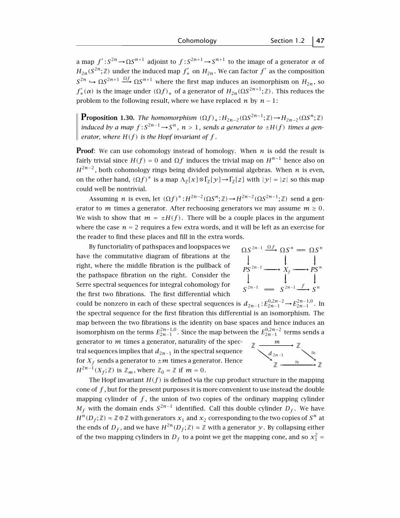
Cohomology Section 1.2 47
a map f ′ :S2n→ΩSn+1 adjoint to f :S2n+1→Sn+1 to the image of a generator α of
H2n(S2n;Z) under the induced map f ′∗ on H2n . We can factor f ′ as the composition
S2n ΩS2n+1 Ωf-----→ΩSn+1 where the first map induces an isomorphism on H2n , so
f ′∗(α) is the image under (Ωf)∗ of a generator of H2n(ΩS2n+1;Z) . This reduces the
problem to the following result, where we have replaced n by n− 1:
Proposition 1.30. The homomorphism (Ωf)∗ :H2n−2(ΩS2n−1;Z)→H2n−2(ΩSn;Z)induced by a map f :S2n−1→Sn , n > 1 , sends a generator to ±H(f) times a gen-
erator, where H(f) is the Hopf invariant of f .
Proof: We can use cohomology instead of homology. When n is odd the result is
fairly trivial since H(f) = 0 and Ωf induces the trivial map on Hn−1 hence also on
H2n−2 , both cohomology rings being divided polynomial algebras. When n is even,
on the other hand, (Ωf)∗ is a map ΛZ[x]⊗ΓZ[y]→ΓZ[z] with |y| = |z| so this map
could well be nontrivial.
Assuming n is even, let (Ωf)∗ :H2n−2(ΩSn;Z)→H2n−2(ΩS2n−1;Z) send a gen-
erator to m times a generator. After rechoosing generators we may assume m ≥ 0.
We wish to show that m = ±H(f) . There will be a couple places in the argument
where the case n = 2 requires a few extra words, and it will be left as an exercise for
the reader to find these places and fill in the extra words.
By functoriality of pathspaces and loopspaces we
have the commutative diagram of fibrations at the
right, where the middle fibration is the pullback of
the pathspace fibration on the right. Consider thePS
−−−−−→−−−−−→
−−−−−→−−−−−→−−−−−→
−−−−−→
n
S -2n 1
S -2n 1
PS -2n 1
f
f
f
===
===Ω −−−−−→−−−−−→
S
S -2n 1
X
ΩΩ −−−−−→−−−−−→
S
S
n
nn Ω
Serre spectral sequences for integral cohomology for
the first two fibrations. The first differential which
could be nonzero in each of these spectral sequences is d2n−1 :E0,2n−22n−1 →E2n−1,0
2n−1 . In
the spectral sequence for the first fibration this differential is an isomorphism. The
map between the two fibrations is the identity on base spaces and hence induces an
isomorphism on the terms E2n−1,02n−1 . Since the map between the E0,2n−2
2n−1 terms sends a
Z Z
Z Z−−−−−→ −−−−−→−−−−−−−−−−−−−−→
−−−−−−−−−−−−−−→≈≈d
m
-2n 1
generator to m times a generator, naturality of the spec-
tral sequences implies that d2n−1 in the spectral sequence
for Xf sends a generator to ±m times a generator. Hence
H2n−1(Xf ;Z) is Zm , where Z0 = Z if m = 0.
The Hopf invariant H(f) is defined via the cup product structure in the mapping
cone of f , but for the present purposes it is more convenient to use instead the double
mapping cylinder of f , the union of two copies of the ordinary mapping cylinder
Mf with the domain ends S2n−1 identified. Call this double cylinder Df . We have
Hn(Df ;Z) ≈ Z⊕Z with generators x1 and x2 corresponding to the two copies of Sn at
the ends of Df , and we have H2n(Df ;Z) ≈ Z with a generator y . By collapsing either
of the two mapping cylinders in Df to a point we get the mapping cone, and so x21 =

48 Chapter 1 The Serre Spectral Sequence
±H(f)y and x22 = ±H(f)y . (In fact the signs are opposite in these two equations
since the homeomorphism of Df switching the two mapping cylinders interchanges
x1 and x2 but takes y to −y .) We also have x1x2 = 0, as can be seen using the cup
product Hn(Df ,A;Z)×Hn(Df ,A;Z)→H2n(Df ,A∪B;Z) , where A and B are the two
mapping cylinders in Df .
There are retractions Df→Sn onto the two copies of Sn in Df . Using one of
these retractions to pull back the path fibration ΩSn→PSn→Sn , we obtain a fibra-
tion ΩSn→Yf→Df . The space Yf is the union of the pullbacks over the two map-
ping cylinders in Df , and these two subfibrations of Yf intersect in Xf . The total
spaces of these two subfibrations are contractible since a deformation retraction of
each mapping cylinder to its target end Sn lifts to a deformation retraction (in the
weak sense) of the subfibration onto PSn which is contractible. The Mayer-Vietoris
sequence for the decomposition of Yf into the two subfibrations then gives isomor-
phisms Hi(Yf ;Z) ≈ Hi−1(Xf ;Z) for all i , so in particular we have H2n(Yf ;Z) ≈ Zm .
Now we look at the Serre spectral sequence for the fibration ΩSn→Yf→Df .
This fibration retracts onto the subfibration
0
1
1
1n
0 n 2n
Z1 Zx 2Zx Zy
Za Zax 2Zax-
⊕
⊕−−−−−→ −−−−−→ΩSn→PSn→Sn over each end of Df . We
know what the spectral sequence for this
subfibration looks like, so by naturality of
the spectral sequence we have da = x1 + x2 for a suitable choice of generator
a of Hn−1(ΩSn;Z) . Then d(ax1) = (x1 + x2)x1 = x21 = ±H(f)y and similarly
d(ax2) = ±H(f)y . Since H2n(Yf ;Z) ≈ Zm it follows that m = ±H(f) . tu
The EHP Spectral Sequence
All the EHP exact sequences of 2 localized homotopy groups can be put together
into a staircase diagram:
−−−→−−−→i 1+ Sπ ( )
S
-n 1
-n 1
-n 2-2n 3
-2n 1
2n 1
-i 1 -i 1 −−−→ −→−→ −−−→ )Sπ ( -Sπ () i 3 Sπ ( )−−−→−−→
−−→−−−→
−−−→−−→
−−→−−−→
−−−→−−→
−−→−−−→ −−−→−−→i 2+ Sπ ( )
S +
n
n
n
−−−→ −→−→ −−−→ )i Sπ ( -iπ () i 2 Sπ ( )
−−→−−→i 3+n 1+
n 1+
n 2+i 1+ i 1+Sπ ( ) −−−→ −→−→ −−−→ )Sπ ( -π (
S
-2n 1
2n 1
2n 3
i 1 )Sπ (
S +
+ )π (
i 3+
i 2+
+
)π ( ) i 1 Sπ ( )
This gives a spectral sequence converging to the stable homotopy groups of
spheres, localized at 2, since these are the groups that occur sufficiently far down each
A column. The E1 page consists of 2 localized homotopy groups of odd-dimensional
spheres. The E2 page has no special form as it does for the Serre spectral sequence,
so one starts by looking at the E1 page. A convenient way to display this is to set
E1k,n = πn+kS2n−1 .
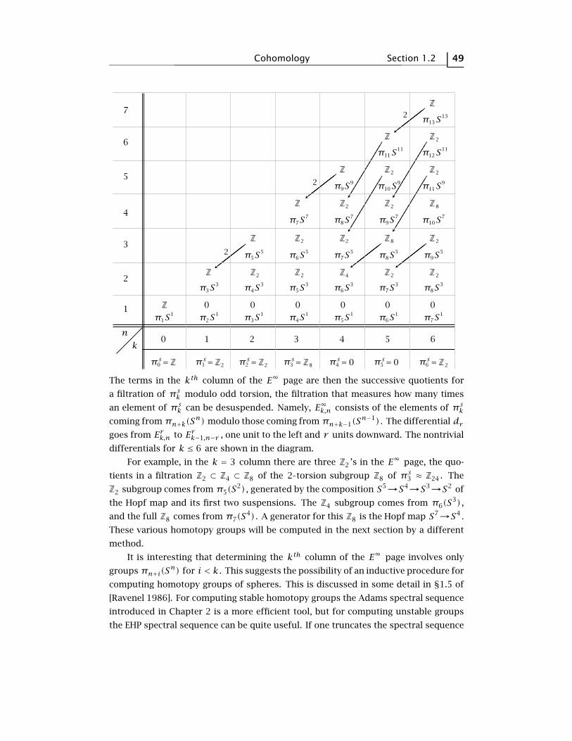
Cohomology Section 1.2 49
−−−−−−−−−−−−−−−→−−−−−−−−−−−−−−−→
−−−−−−−−−−−−−−−→
−−−−−−−−−−−−−−−→
−−−−−−−−−−−−−−−→
−−−−−−−−−−−−−−−→
−−−−−−−−−−−−−−−→
−−−−−−−−−−−−−−−→
−−−−−−−−−−−−−−−→
S11π
0sπ
S12
2 2 4 2 2
π S13π S14π S15π S16π S17π
S33π S
k0 1
1
2
3
4
5
6
7
2
2
2
2
3 4 5 6n
34π S35π S36π S37π S38π
S55π S56π S57π S58π S59π
S77π S78π S79π S710π
S99π S910π S911π
S1111π S1112π
S1313π
Z
Z
0 0 0 0 0 0
Z Z Z Z Z Z
2 2 8 2Z Z Z Z Z
2 2 8Z Z Z Z
2 2Z Z Z
2Z Z
Z
= 1sπ Z= 2 22 8
sπ Z= 3sπ Z= 4
sπ 0= 5sπ 0= 6 2
sπ Z=
The terms in the kth column of the E∞ page are then the successive quotients for
a filtration of πsk modulo odd torsion, the filtration that measures how many times
an element of πsk can be desuspended. Namely, E∞k,n consists of the elements of πskcoming from πn+k(S
n) modulo those coming from πn+k−1(Sn−1) . The differential dr
goes from Erk,n to Erk−1,n−r , one unit to the left and r units downward. The nontrivial
differentials for k ≤ 6 are shown in the diagram.
For example, in the k = 3 column there are three Z2 ’s in the E∞ page, the quo-
tients in a filtration Z2 ⊂ Z4 ⊂ Z8 of the 2 torsion subgroup Z8 of πs3 ≈ Z24 . The
Z2 subgroup comes from π5(S2) , generated by the composition S5→S4→S3→S2 of
the Hopf map and its first two suspensions. The Z4 subgroup comes from π6(S3) ,
and the full Z8 comes from π7(S4) . A generator for this Z8 is the Hopf map S7→S4 .
These various homotopy groups will be computed in the next section by a different
method.
It is interesting that determining the kth column of the E∞ page involves only
groups πn+i(Sn) for i < k . This suggests the possibility of an inductive procedure for
computing homotopy groups of spheres. This is discussed in some detail in §1.5 of
[Ravenel 1986]. For computing stable homotopy groups the Adams spectral sequence
introduced in Chapter 2 is a more efficient tool, but for computing unstable groups
the EHP spectral sequence can be quite useful. If one truncates the spectral sequence

50 Chapter 1 The Serre Spectral Sequence
by replacing all rows above the nth row with zeros, one obtains a spectral sequence
converging to π∗(Sn) . In the staircase diagram this amounts to replacing all the
exact sequences below a given one with trivial exact sequences having E terms zero
and isomorphic pairs of A terms.
Odd Torsion
In the case that the EHP sequence is valid at all primes, it in fact splits at odd
primes:
Proposition 1.31. After factoring out 2 torsion there are isomorphisms
πi(Sn) ≈ πi−1(S
n−1)⊕πi(S2n−1) for all even n .
Thus, apart from 2 torsion, the homotopy groups of even dimensional spheres
are determined by those of odd-dimensional spheres. For Z summands we are already
familiar with the splitting, as the only Z ’s in the right side occur when i is n and
2n− 1.
Proof: Given a map f :S2n−1→Sn , consider the map i · Ωf :Sn−1×ΩS2n−1 -→ΩSnobtained by multiplying the inclusion map i :Sn−1 ΩSn and the map Ωf , using
the H–space structure on ΩSn . Taking f to have H(f) = ±2 in the case that nis even, for example taking f = [ι, ι] , the preceding Proposition 1.30 implies that
the map i · Ωf induces an isomorphism on cohomology with Z[1/2] coefficients in
all dimensions. The same is therefore true for homology with Z[1/2] coefficients and
therefore also for homotopy groups tensored with Z[1/2] by Theorem 1.23 since we
are dealing with spaces that are simply-connected if n > 2, or abelian if n = 2. tu
When n = 2,4,8 we can modify the proof by taking f to have Hopf invariant ±1,
and then i·Ωf will induce an isomorphism on homology with Z coefficients and hence
be a homotopy equivalence, so in these cases the splitting holds without factoring out
2 torsion. However there is a much simpler derivation of these stronger splittings
using the Hopf bundles Sn−1→S2n−1→Sn since a nullhomotopy of the inclusion
Sn−1S2n−1 gives rise to a splitting of the long exact sequence of homotopy groups
of the bundle. This can be interpreted as saying that if we continue the Hopf bundle
to a fibration sequence
ΩS2n−1→ΩSn→Sn−1→S2n−1→Snthen we obtain a product two stages back from the Hopf bundle.
The EHP spectral sequence we constructed for 2 torsion has an analog for odd
primary torsion, but the construction is a little more difficult. This is described in
[Ravenel 1986].

Cohomology Section 1.2 51
Exercises
1. Use the Serre spectral sequence to compute H∗(F ;Z) for F the homotopy fiber of
a map Sk→Sk of degree n for k,n > 1, and show that the cup product structure in
H∗(F ;Z) is trivial.
2. For a fibration F i-----→ X p-----→ B with B path-connected, show that if the map
i∗ :H∗(X;G)→H∗(F ;G) is surjective then:
(a) The action of π1(B) on H∗(F ;G) is trivial.
(b) All differentials originating in the left-hand column of the Serre spectral sequence
for cohomology are zero.
3. Let F i-----→X p-----→B be a fibration with B path-connected. The Leray-Hirsch theorem,
proved in §4.D of [AT] without using spectral sequences, asserts that if Hk(F ;R) is
a finitely-generated free R module for each k and there exist classes cj ∈ H∗(X;R)whose images under i∗ form a basis for H∗(F ;R) , then H∗(X;R) , regarded as a
module over H∗(B;R) , is free with basis the classes cj . This is equivalent to saying
that the map H∗(F ;R)⊗RH∗(B;R)→H∗(X;R) sending i∗(cj)⊗b to cj ` p∗(b) is
an isomorphism of H∗(B;R) modules. (It is not generally a ring isomorphism.) The
coefficient ring R can be any commutative ring, with an identity element of course.
Show how this theorem can be proved using the Serre spectral sequence. [Use the
preceding problem. The freeness hypothesis gives Ep,q2 ≈ Ep,02 ⊗RE0,q2 . Deduce that all
differentials must be trivial so E2 = E∞ . The final step is to go from E∞ to H∗(X;R) .]

52 Chapter 1 The Serre Spectral Sequence
1.3 Eilenberg-MacLane Spaces
The only Eilenberg-MacLane spaces K(π,n) with n > 1 whose homology and
cohomology can be computed by elementary means are K(Z,2) ' CP∞ and a product
of copies of K(Z,2) , which is a K(π,2) with π free abelian. Using the Serre spectral
sequence we will now go considerably beyond this and compute H∗(K(Z2, n);Z2) .[It is possible to go further in the same direction and compute H∗(K(Zp,n);Zp)
for p an odd prime, but the technical details are significantly more complicated, so
we postpone this until later — either a later version of this chapter or a later chapter
using the Eilenberg-Moore spectral sequence. In the meantime a reference for this is
[McCleary 2001], Theorem 6.19.]
Computing H∗(K(Z2, n);Z2) is equivalent to determining all cohomology opera-
tions with Z2 coefficients, so it should not be surprising that Steenrod squares play a
central role in the calculation. We will assume the reader is at least familiar with the
basic axioms for Steenrod squares, as developed for example in §4.L of [AT]:
(1) Sqi(f∗(α)) = f∗(Sqi(α)) for f :X→Y .
(2) Sqi(α+ β) = Sqi(α)+ Sqi(β) .(3) Sqi(α` β) =∑j Sqj(α)` Sqi−j(β) (the Cartan formula).
(4) Sqi(σ(α)) = σ(Sqi(α)) where σ :Hn(X;Z2)→Hn+1(ΣX;Z2) is the suspension
isomorphism given by reduced cross product with a generator of H1(S1;Z2) .(5) Sqi(α) = α2 if i = |α| , and Sqi(α) = 0 if i > |α| .(6) Sq0 = 11, the identity.
(7) Sq1 is the Z2 Bockstein homomorphism β associated with the coefficient se-
quence 0→Z2→Z4→Z2→0.
We will not actually use all these properties, and in particular not the most compli-
cated one, the Cartan formula. It would in fact be possible to do the calculation of
H∗(K(Z2, n);Z2) without using Steenrod squares at all, and then use the calculation
to construct the squares and prove the axioms, but since this only occupied five pages
in [AT] and would take a similar length to rederive here, it hardly seems worth the
effort.
In order to state the main result we need to recall some notation and terminology
involving Steenrod squares. The monomial Sqi1 ···Sqik , which is the composition
of the individual operations Sqij , is denoted SqI where I = (i1, ··· , ik) . It is a fact
that any SqI can be expressed as a linear combination of admissible SqI ’s, those for
which ij ≥ 2ij+1 for each j . This will follow from the main theorem, and explicit
formulas are given by the Adem relations. The excess of an admissible SqI is e(I) =∑j(ij−2ij+1) , giving a measure of how much SqI exceeds being admissible. The last
term of this summation is ik − 2ik+1 = ik via the convention that adding zeros at the
end of an admissible sequence (i1, ··· , ik) does not change it, in view of the fact that
Sq0 is the identity.

Eilenberg-MacLane Spaces Section 1.3 53
Here is the theorem, first proved by Serre as one of the early demonstrations of
the power of the new spectral sequence.
Theorem 1.32. H∗(K(Z2, n);Z2) is the polynomial ring Z2[SqI(ιn)] where ιn is a
generator of Hn(K(Z2, n);Z2) and I ranges over all admissible sequences of excess
e(I) < n .
When n = 1 this is the familiar result that H∗(K(Z2,1);Z2) is the polynomial
ring Z2[ι1] since the only admissible SqI with excess 0 is Sq0 . The admissible SqI ’sof excess 1 are Sq1 , Sq2Sq1 , Sq4Sq2Sq1 , Sq8Sq4Sq2Sq1 , ··· , so when n = 2 the
theorem says that H∗(K(Z2,1);Z2) is the polynomial ring on the infinite sequence of
generators ι2 , Sq1(ι2) , Sq2Sq1(ι2) , ··· . For larger n there are even more generators,
but still only finitely many in each dimension, as must be the case since K(Z2, n) has
finitely generated homotopy groups and hence finitely generated cohomology groups.
What is actually happening when we go from K(Z2, n) to K(Z2, n+ 1) is that all the
2j th powers of all the polynomial generators for H∗(K(Z2, n);Z2) shift up a dimen-
sion and become new polynomial generators for H∗(K(Z2, n + 1);Z2) . For example
when n = 1 we have a single polynomial generator ι1 , whose powers ι1 , ι21 = Sq1(ι1) ,ι41 = Sq2Sq1(ι1) , ι
81 = Sq4Sq2Sq1(ι1) , ··· shift up a dimension to become the polyno-
mial generators ι2 , Sq1(ι2) , Sq2Sq1(ι2) , ··· for H∗(K(Z2,2);Z2) . At the next stage
one would take all the 2j th powers of these generators and shift them up a dimension
to get the polynomial generators for H∗(K(Z2,3);Z2) , and so on for each successive
stage. The mechanics of how this works is explained by part (b) of the following
lemma. Parts (a) and (b) together explain the restriction e(I) < n in the theorem.
Lemma 1.33. (a) SqI(ιn) = 0 if SqI is admissible and e(I) > n .
(b) The elements SqI(ιn) with SqI admissible and e(I) = n are exactly the powers(SqJ(ιn)
)2j with J admissible and e(J) < n .
Proof: For a monomial SqI = Sqi1 ···Sqik the definition of e(I) can be rewritten as
an equation i1 = e(I)+i2+i3+···+ik . Thus if e(I) > n we have i1 > n+i2+···+ik =|Sqi2 ···Sqik(ιn)| , hence SqI(ιn) = 0.
If e(I) = n then i1 = n + i2 + ··· + ik so SqI(ιn) =(Sqi2 ···Sqik(ιn)
)2 . Since
SqI is admissible we have e(i2, ··· , ik) ≤ e(I) = n , so either Sqi2 ···Sqik has ex-
cess less than n or it has excess equal to n and we can repeat the process to write
Sqi2 ···Sqik(ιn) =(Sqi3 ··· (ιn)
)2 , and so on, until we obtain an equation SqI(ιn) =(SqJ(ιn)
)2j with e(J) < n .
Conversely, suppose that Sqi2 ···Sqik is admissible with e(i2, ··· , ik) ≤ n , and
let i1 = n + i2 + ··· + ik so that Sqi1Sqi2 ···Sqik(ιn) =(Sqi2Sqi3 ··· (ιn)
)2 . Then
(i1, ··· , ik) is admissible since e(i2, ··· , ik) ≤ n implies i2 ≤ n+ i3 + ··· + ik hence
i1 = n+ i2+···+ ik ≥ 2i2 . Furthermore, e(i1, ··· , ik) = n since i1 = n+ i2+···+ ik .
Thus we can iterate to express a 2j th power of an admissible SqJ(ιn) with e(J) < nas an admissible SqI(ιn) with e(I) ≤ n . tu

54 Chapter 1 The Serre Spectral Sequence
The proof of Serre’s theorem will be by induction on n using the Serre spec-
tral sequence for the path fibration K(Z2, n)→P→K(Z2, n + 1) . The key ingredient
for the induction step is a theorem due to Borel. The statement of Borel’s theorem
involves the notion of transgression which we introduced at the end of §1.1 in the
case of homology, and the transgression for cohomology is quite similar. Namely,
in the cohomology Serre spectral sequence of a fibration F→X→B the differential
dr :E0,r−1r →Er,0r from the left edge to the bottom edge is call the transgression τ .
This has domain a subgroup of Hr−1(F) , the elements on which the previous differ-
entials d2, ··· , dr−1 are zero. Such elements are called transgressive. The range of
τ is a quotient of Hr(B) , obtained by factoring out the images of d2, ··· , dr−1 . Thus
if an element x ∈ H∗(F) is transgressive, then τ(x) is strictly speaking a coset in
H∗(B) , but we will often be careless with words and not distinguish between the coset
and a representative element.
Here is Borel’s theorem:
Theorem 1.34. Let F→X→B be a fibration with X contractible and B simply-
connected. Suppose that the cohomology H∗(F ;k) with coefficients in a field k has
a basis consisting of all the products xi1 ···xik of distinct transgressive elements
xi ∈ H∗(F ;k) , only finitely many of which lie in any single Hj(F ;R) and which are
odd-dimensional if the characteristic of k is not 2 . Then H∗(B;k) is the polynomial
algebra k[··· , yi, ···] on elements yi representing the transgressions τ(xi) .
Elements xi whose distinct products form a basis for H∗(F ;k) are called a simple
system of generators. For example, an exterior algebra obviously has a simple system
of generators. A polynomial algebra k[x] also has a simple system of generators, the
powers x2i . The same is true for a truncated polynomial algebra k[x]/(x2i ) . The
property of having a simple system of generators is clearly preserved under tensor
products, so for example a polynomial ring in several variables has a simple system
of generators.
Here are a few more remarks on the theorem:
If the characteristic of k is not 2 the odd-dimensional elements xi in the theorem
have x2i = 0 so H∗(F ;k) is in fact an exterior algebra in this case.
Contractibility of X implies that F has the weak homotopy type of ΩB , by Propo-
sition 4.66 of [AT]. Then by §3.C of [AT] H∗(F ;k) is a Hopf algebra, the tensor
product of exterior algebras, polynomial algebras, and truncated polynomial al-
gebras k[xpi] where p is the characteristic of k . Hence in many cases H∗(F ;k)
has a simple system of generators.
Another theorem of Borel asserts that H∗(B;k) is a polynomial algebra on even-
dimensional generators if and only if H∗(F ;k) is an exterior algebra on odd-
dimensional generators, without any assumptions about transgressions. Borel’s
original proof involved a detailed analysis of the Serre spectral sequence, but we

Eilenberg-MacLane Spaces Section 1.3 55
will give a more conceptual proof in Chapter 3 using the Eilenberg-Moore spectral
sequence.
In order to find enough transgressive elements to apply Borel’s theorem to in the
present context we will use the following technical fact:
Lemma 1.35. If x ∈ H∗(F ;Z2) is transgressive then so is Sqi(x) , and τ(Sqi(x)) =Sqi(τ(x)) .
Proof: The analog of Proposition 1.13 for cohomology, proved in just the same way,
says that τ is the composition j∗(p∗)−1δ in
the diagram at the right. For x to be transgres- −−−−−→ −−−−−→−−−−−→
bBH H( ) B( ),
FXHr( ),FH
rr
( )-r 1
p∗
j∗
δsive means that δx lies in the image of p∗ , so
the same holds for Sqi(x) by naturality and
the fact that Sqi commutes with δ since it commutes with suspension and δ can
be defined in terms of suspension. The relation τ(Sqi(x)) = Sqi(τ(x)) then also
follows by naturality. tu
Proof of Serre’s theorem, assuming Borel’s theorem: This is by induction on n start-
ing from the known case K(Z2,1) . For the induction step we use the path fibration
K(Z2, n)→P→K(Z2, n + 1) . When n = 1 the fiber is K(Z2,1) with the simple sys-
tem of generators ι2i
1 = Sq2i−1 ···Sq2Sq1(ι1) . These are transgressive by the lemma
since ι1 is obviously transgressive with τ(ι1) = ι2 . So Borel’s theorem says that
H∗(K(Z2,2);Z2) is the polynomial ring on the generators Sq2i ···Sq2Sq1(ι2) .The general case is similar. If H∗(K(Z2, n);Z2) is the polynomial ring in the ad-
missible SqI(ιn) ’s with e(I) < n then it has a simple system of generators consisting
of the 2i th powers of these SqI(ιn) ’s, i = 0,1, ··· . By Lemma 1.33 these powers are
just the admissible SqI(ιn) ’s with e(I) ≤ n . These elements are transgressive since
ιn is transgressive, the spectral sequence having zeros between the 0th and nth rows.
Since τ(ιn) = ιn+1 , we have τ(SqI(ιn)) = SqI(ιn+1) , and Borel’s theorem gives the
desired result for K(Z2, n+ 1) . tu
Proof of Borel’s Theorem: The idea is to build an algebraic model of what we would
like the Serre spectral sequence of the fibration to look like, then use the spectral
sequence comparison theorem to show that this model is correct.
The basic building block for the model is a spectral sequence Ep,qr (i) pictured
below, whose E2 page is a tensor product Λk[xi]⊗k[yi] where xi and yi have the
same dimensions as xi and yi .
1 y 2 . . .3
x 2−−−−−−−−−−−−→−−−−−−−−−−−−→
−−−−−−−−−−−−→−
−
⊗
i y−i y−i
i x−i y−i ⊗x−i y−i . . .

56 Chapter 1 The Serre Spectral Sequence
The nontrivial differentials are the only ones which could be nonzero, indicated by the
arrows, namely dr(xi ⊗ymi ) = ym+1i for r = |yi| . Hence the E∞ page consists of just
a k in the (0,0) position. We then get the model spectral sequence we are looking for
by setting Ep,qr = ⊗iEp,qr (i) . With differentials defined by the usual boundary formula
in a tensor product, this is also a spectral sequence, in the sense that passing from
Er to Er+1 is achieved by taking homology with respect to the r th differential. This
is because we can regard Er as a chain complex by taking the sum of the terms along
each diagonal p + q = n , and over a field the homology of a tensor product of chain
complexes is the tensor product of the homologies.
If the Serre spectral sequence for the given fibration is denoted Ep,qr , we may
define a map Φ :Ep,q2 →Ep,q2 by xi, xi and yi, yi , extending multiplicatively
to products of these generators. Note that Φ is only an additive homomorphism
since in Λk[xi] we have x2i = 0 but it need not be true that x2
i = 0 in the case
k = Z2 that we need for the proof of Serre’s theorem. The hypothesis that the xi ’stransgress to the yi ’s guarantees that Φ is a map of spectral sequences, commuting
with differentials. Since the total space X is contractible, Φ is an isomorphism on
the E∞ pages. The assumption that the xi are a simple system of generators implies
that Φ is an isomorphism E0,q2 ≈ E0,q
2 . The algebraic form of the spectral sequence
comparison theorem (see below) then says that Φ is an isomorphism Ep,02 ≈ Ep,02 . On
this row of the E2 page Φ is a ring homomorphism since its domain is a polynomial
ring and we have sent the generators for this ring to the yi ’s. The result follows. tu
Here is the form of the spectral sequence comparison theorem for cohomology.
Theorem 1.36. Suppose we have a map Φ between two first quadrant spectral se-
quences of cohomological type, so dr goes from Ep,qr to Ep+r ,q−r+1r . Assume that
Ep,q2 = Ep,02 ⊗E0,q2 for both spectral sequences. Then any two of the following three
conditions imply the third:
(i) Φ is an isomorphism on the Ep,02 terms.
(ii) Φ is an isomorphism on the E0,q2 terms.
(iii) Φ is an isomorphism on the E∞ page.
The fact that (i) and (ii) imply (iii) is easy since they imply that Φ is an isomorphism
on E2 , hence on each subsequent page as well. The other two implications take more
work. The proofs are similar, and we shall do just the one we need here.
Proof that (ii) and (iii) imply (i): Assume inductively that Φ is an isomorphism on
Ep,02 for p ≤ k . We shall first show that this together with (ii) implies:
(a) Φ is an isomorphism on Ep,qr for p ≤ k− r + 1.
(b) Φ is injective on Ep,qr for p ≤ k .
This is by induction on r . Both assertions are certainly true for r = 2. For the
induction step, assume they are true for r . Let Zp,qr and Bp,qr be the subgroups of

Eilenberg-MacLane Spaces Section 1.3 57
Ep,qr that are the kernel and image of dr , in other words the cycles and boundaries,
so Ep,qr+1 = Zp,qr /Bp,qr . First we show (a) for Ep,qr+1 .
(1) From the exact sequence
0 -→Zp,qr -→Ep,qrdr-----→Ep+r ,q−r+1
r
we deduce that Φ is an isomorphism on Zp,qr for p ≤ k − r since by (a) it is an
isomorphism on Ep,qr for p ≤ k − r + 1 and by (b) it is injective on Ep+r ,q−r+1r for
p + r ≤ k , that is, p ≤ k− r .
(2) The exact sequence
Ep−r ,q+r−1r
dr-----→Ep,qr -→Ep,qr /Bp,qr -→0
shows that Φ is an isomorphism on Ep,qr /Bp,qr for p ≤ k − r + 1 since by (a) it is an
isomorphism on Ep,qr for p ≤ k− r + 1 and on Ep−r ,q+r−1r for p − r ≤ k− r + 1, or
p ≤ k+ 1.
(3) From the preceding step and the short exact sequence
0 -→Bp,qr -→Ep,qr -→Ep,qr /Bp,qr -→0
we conclude that Φ is an isomorphism on Bp,qr for p ≤ k− r + 1.
(4) From steps (1) and (3) and the short exact sequence
0 -→Bp,qr -→Zp,qr -→Ep,qr+1 -→0
we see that Φ is an isomorphism on Ep,qr+1 for p ≤ k − r , or in other words, p ≤k− (r + 1)+ 1, which finishes the induction step for (a).
For (b), induction gives that Φ is injective on Zp,qr if p ≤ k . From exactness of
Ep−r ,q+r−1r →Bp,qr →0 we deduce using (a) that Φ is surjective on Bp,qr for p − r ≤k − r + 1, or p ≤ k + 1. Then the exact sequence in (4) shows that Φ is injective on
Ep,qr+1 if p ≤ k .
Returning now to the main line of the proof, we will show that Φ is an isomor-
phism on Ek+1,02 using the exact sequence
Zk−r+1,r−1r -→Ek−r+1,r−1
rdr-----→Ek+1,0
r -→Ek+1,0r+1 -→0
We know that Φ is an isomorphism on Ek−r+1,r−1r by (a). We may assume Φ is an
isomorphism on Ek+1,0r+1 by condition (iii) and downward induction on r . If we can
show that Φ is surjective on Zk−r+1,r−1r then the five lemma will imply that Φ is an
isomorphism on Ek+1,0r and the proof will be done.
We show that Φ is surjective on Zk−r+1,r−1s for s ≥ r by downward induction on
s . Consider the five-term exact sequence
Zk−r−s+1,r+s−2s -→Ek−r−s+1,r+s−2
sds-----→Zk−r+1,r−1
s -→Ek−r+1,r−1s+1 -→0
On the second term Φ is an isomorphism by (a). The fourth term Ek−r+1,r−1s+1 is the
same as Zk−r+1,r−1s+1 since ds+1 is zero on this term if s ≥ r . Downward induction on

58 Chapter 1 The Serre Spectral Sequence
s then says that Φ is surjective on this term. Applying one half of the five lemma, the
half involving surjectivity, yields the desired conclusion that Φ is surjective on the
middle term Zk−r+1,r−1s . tu
The technique used to prove Serre’s theorem works without further modification
in two other cases as well:
Theorem 1.37. (a) H∗(K(Z, n);Z2) for n > 1 is the polynomial ring on the gener-
ators SqI(ιn) as SqI ranges over all admissible monomials of excess e(I) < n and
having no Sq1 term.
(b) H∗(K(Z2k , n);Z2) for k > 1 and n > 1 is the polynomial ring on generators
SqI(ιn) and SqI(κn+1) as SqI ranges over all admissible monomials having no Sq1
term, with e(I) < n for SqI(ιn) and e(I) ≤ n for SqI(κn+1) . Here κn+1 is a
generator of Hn+1(K(Z2k , n);Z2) ≈ Z2 .
If k were 1 in part (b) then κn+1 would be Sq1(ιn) , but for k > 1 we have
Sq1(ιn) = 0 since Sq1 is the Z2 Bockstein and ιn is the Z2 reduction of a Z4 class.
Thus a new generator κn+1 is needed. Nevertheless, the polynomial ring in (b) is
isomorphic as a graded ring to H∗(K(Z2, n);Z2)˚by replacing κn+1 by Sq1(ιn) .
Proof: For part (a) the induction starts with n = 2 where H∗(K(Z,2);Z2) = Z2[ι2]with a simple system of generators ι2 , ι22 = Sq2ι2 , ι42 = Sq4Sq2ι2 , ··· . This implies
that for n = 3 one has polynomials on the generators ι3 , Sq2(ι3) , Sq4Sq2(ι3) , ··· ,
and so on for higher values of n .
For (b), when n = 1 and k > 1 the lens space calculations in [AT] show that
H∗(K(Z2k ,1);Z2) is ΛZ2[ι1]⊗Z2[κ2] rather than a pure polynomial algebra. A simple
system of generators is ι1 , κ2 , κ22 = Sq2(κ2) , κ
42 = Sq4Sq2(κ2) , ··· , and both ι1
and κ2 are transgressive, transgressing to ι2 and κ3 , so Borel’s theorem says that for
n = 2 one has the polynomial ring on generators ι2 , κ3 , Sq2(κ3) , Sq4Sq2(κ3) , ··· .
The inductive step for larger n is similar. tu
Using these results and the fact that K(Zpk,n) has trivial Z2 cohomology for pan odd prime, one could apply the Kunneth formula to compute the Z2 cohomology
of any K(π,n) with π a finitely generated abelian group.
Relation with the Steenrod Algebra
The Steenrod algebra A2 can be defined as the algebra generated by the Sqi ’ssubject only to the Adem relations. This is a graded algebra, with SqI having degree
d(I) =∑j ij , the amount by which the operation SqI raises dimension.
Corollary 1.38. The map A2→H∗(K(Z2, n);Z2) , SqI,SqI(ιn) , is an isomorphism
from the degree d part of A2 onto Hn+d(K(Z2, n);Z2) for d ≤ n . In particular, the
admissible monomials SqI form an additive basis for A2 .

Eilenberg-MacLane Spaces Section 1.3 59
Proof: The map is surjective since Hn+d(K(Z2, n);Z2) for d < n consists only of
linear polynomials in the SqI(ιn) ’s, and the only nonlinear term for d = n is ι2n =Sqn(ιn) . For injectivity, note first that d(I) ≥ e(I) , and Sqn is the only monomial
with degree and excess both equal to n . So the admissible SqI with d(I) ≤ n map
to linearly independent classes in H∗(K(Z2, n);Z2) . Since the Adem relations allow
any monomial to be expressed in terms of admissible monomials, injectivity follows,
as does the linear independence of the admissible monomials. tu
One can conclude that A2 is exactly the algebra of all Z2 cohomology operations
that are stable, commuting with suspension. Since general cohomology operations
correspond exactly to cohomology classes in Eilenberg-MacLane spaces, the algebra
of stable Z2 operations is the inverse limit of the sequence
··· -→H∗(K(Z2, n+ 1);Z2) -→H∗(K(Z2, n);Z2) -→···where the maps are induced by maps fn :ΣK(Z2, n)→K(Z2, n+1) that induce an iso-
morphism on πn+1 , together with the suspension isomorphisms Hi(K(Z2, n);Z2) ≈Hi+1(ΣK(Z2, n);Z2) . Since fn induces an isomorphism on homotopy groups through
dimension approximately 2n by the Freudenthal suspension theorem, Corollary 4.24
in [AT], it also induces isomorphisms on homology and cohomology in this same ap-
proximate dimension range, so the inverse limit is achieved at finite stages in each
dimension.
Unstable operations do exist, for example x, x3 for x ∈ H1(X;Z2) . This cor-
responds to the element ι31 ∈ H3(K(Z2,1);Z2) , which is not obtainable by applying
any element of A2 to ι1 , the only possibility being Sq2 but Sq2(ι1) is zero since ι1 is
1 dimensional. According to Serre’s theorem, all unstable operations are polynomials
in stable ones.
Integer Coefficients
It is natural to ask about the cohomology of K(Z2, n) with Z coefficients. Since the
homotopy groups are finite 2 groups, so are the reduced homology and cohomology
groups with Z coefficients, and the first question is whether there are any elements
of order 2k with k > 1. For n = 1 the answer is certainly no since RP∞ is a K(Z2,1) .For larger n it is also true that Hj(K(Z2, n);Z) contains only elements of order 2
if j ≤ 2n . This can be shown using the Bockstein β = Sq1 , as follows. Using the
Adem relations Sq1Sq2i = Sq2i+1 and Sq1Sq2i+1 = 0 we see that applying β to
an admissible monomial Sqi1Sqi2 ··· gives the admissible monomial Sqi1+1Sqi2 ···when i1 is even and 0 when i1 is odd. Hence in A2 we have Kerβ = Imβ with basis
the admissible monomials beginning with Sq2i+1 . This implies that Kerβ = Imβ in
Hj(K(Z2, n);Z2) for j < 2n , so by the general properties of Bocksteins explained in
§3.E of [AT] this implies that Hj(K(Z2, n);Z) has no elements of order greater than
2 for j ≤ 2n .

60 Chapter 1 The Serre Spectral Sequence
However if n is even then Kerβ/ Imβ in H2n(K(Z2, n);Z2) is Z2 generated by
the element Sqn(ιn) = ι2n . Hence H2n+1(K(Z2, n);Z) contains exactly one summand
Z2k with k > 1. The first case is n = 2, and here we will compute explicitly in §??
that H5(K(Z2,2);Z) = Z4 . In the general case of an arbitrary even n the universal
coefficient theorem implies that H2n+1(K(Z2, n);Z4) contains a single Z4 summand.
This corresponds to a cohomology operation Hn(X;Z2)→H2n(X;Z4) called the Pon-
tryagin square.
A full description of the cohomology of K(Z2, n) with Z coefficients can be deter-
mined by means of the Bockstein spectral sequence. This is worked out in Theorem
10.4 of [May 1970]. The answer is moderately complicated.
Cell Structure
Serre’s theorem allows one to determine the minimum number of cells of each
dimension in a CW complex K(Z2, n) . An obvious lower bound on the number of
k cells is the dimension of Hk(K(Z2, n);Z2) as a vector space over Z2 , and in fact
there is a CW complex K(Z2, n) that realizes this lower bound for all k . This is
evident for n = 1 since RP∞ does the trick. For n > 1 we are dealing with a simply-
connected space so Proposition 4C.1 in [AT] says that there is a CW complex K(Z2, n)having the minimum number of cells compatible with its Z homology, namely one cell
for each Z summand of its Z homology, which in this case occurs only in dimension
0, and two cells for each finite cyclic summand. Each finite cyclic summand of the Z
homology has order a power of 2 and gives two Z2 ’s in the Z2 cohomology, so the
result follows.
For example, for K(Z2,2) the minimum number of cells of dimensions 2,3, ··· ,10
is, respectively, 1,1,1,2,2,2,3,4,4. The numbers increase, but not too rapidly, a
pleasant surprise since the general construction of a K(π,n) by killing successive
homotopy groups might lead one to expect that rather large numbers of cells would
be needed even in fairly low dimensions.
Pontryagin Ring Structure
Eilenberg-MacLane spaces K(π,n) with π abelian are H–spaces since they are
loopspaces, so their cohomology rings with coefficients in a field are Hopf algebras.
Serre’s theorem allows the Hopf algebra structure in H∗(K(Z2, n);Z2) to be deter-
mined very easily, using the following general fact:
Lemma 1.39. If X is a path-connected H–space and x ∈ H∗(X;Z2) is primitive, then
so is Sqi(x) .
Proof: For x to be primitive means that ∆(x) = x ⊗1+1⊗x where ∆ is the coproduct
in the Hopf algebra structure, the map
H∗(X;Z2)µ∗------------→H∗(X×X;Z2) ≈ H∗(X;Z2)⊗H∗(X;Z2)

Eilenberg-MacLane Spaces Section 1.3 61
where µ :X×X→X is the H–space multiplication and the isomorphism is given by
cross product. For a general x we have ∆(x) =∑i x′i ⊗x′′i , or in other words, µ∗(x) =∑i x′i×x′′i . The total Steenrod square Sq = 1+Sq1+Sq2+··· is a ring homomorphism
by the Cartan formula, and by naturality this is equivalent to the cross product formula
Sq(a×b) = Sq(a)×Sq(b) . So if x is primitive we have
µ∗Sq(x) = Sq(µ∗(x)) = Sq(x×1+ 1×x)= Sq(x)×Sq(1)+ Sq(1)×Sq(x) = Sq(x)×1+ 1×Sq(x)
which says that µ∗Sqi(x) = Sqi(x)×1+ 1×Sqi(x) , so Sqi(x) is primitive. tu
By Serre’s theorem, H∗(K(Z2, n);Z2) is then generated by primitive elements
SqI(ιn) . In a Hopf algebra generated by primitives the coproduct is uniquely de-
termined by the product, since the coproduct is an algebra homomorphism. This
means that we can say that H∗(K(Z2, n);Z2) as a Hopf algebra is the tensor product
of one-variable polynomial algebras Z2[SqI(ιn)] . It follows as in §3.C of [AT] that
the dual Pontryagin algebra H∗(K(Z2, n);Z2) is the tensor product of divided poly-
nomial algebras ΓZ2[αI] on the homology classes αI dual to the SqI(ιn) ’s. Since a
divided polynomial algebra over Z2 is actually an exterior algebra, we can also say
that H∗(K(Z2, n);Z2) , regarded just as an algebra and ignoring its coproduct, is an
exterior algebra on the homology classes dual to the powers(SqI(ιn)
)2j as I ranges
over admissible monomials of excess e(I) < n . By Lemma 1.33 we could just as well
say the exterior algebra on the homology classes dual to the elements SqI(ιn) as Iranges over admissible monomials of excess e(I) ≤ n .
Computing Homotopy Groups of Spheres
Using information about cohomology of Eilenberg-MacLane spaces one can at-
tempt to compute a Postnikov tower for Sn and in particular determine its homotopy
groups. To illustrate how this technique works we shall carry it out just far enough
to compute πn+i(Sn) for i ≤ 3. We already know that πn+1(S
n) is Z for n = 2 and
Z2 for n ≥ 3. Here are the next two cases:
Theorem 1.40. (a) πn+2(Sn) = Z2 for n ≥ 2 .
(b) π5(S2) = Z2 , π6(S
3) = Z12 , π7(S4) = Z⊕Z12 , and πn+3(S
n) = Z24 for n ≥ 5 .
In the course of the proof we will need a few of the simpler Adem relations in
order to compute some differentials. For convenience we list these relations here:
Sq1Sq2n = Sq2n+1, Sq1Sq2n+1 = 0
Sq2Sq2 = Sq3Sq1, Sq3Sq2 = 0, Sq2Sq3 = Sq5 + Sq4Sq1, Sq3Sq3 = Sq5Sq1
Proof: By Theorem 1.28 all the torsion in these groups is 2 torsion except for a Z3
in πn+3(Sn) for n ≥ 3. This will allow us to focus on cohomology with Z2 coeffi-
cients, but we will also need to use Z coefficients to some extent. When we do use

62 Chapter 1 The Serre Spectral Sequence
Z coefficients we will be ignoring odd torsion, whether we say this explicitly or not.
Alternatively we could localize all the spaces at the prime 2. This is perhaps more
elegant, but not really necessary.
Since πn(S2) ≈ πn(S3) for n ≥ 3 via the Hopf bundle, we may start with S3 .
A Postnikov tower for S3 consists of fibrations K(πn(S3),n)→Xn→Xn−1 , starting
with X3 = K(Z,3) . The spaces Xn come with maps S3→Xn , and thinking of these as
inclusions via mapping cylinders, the pairs (Xn, S3) are (n+1) connected since up to
homotopy equivalence we can build Xn from S3 by attaching cells of dimension n+2
and greater to kill πn+1 and the higher homotopy groups. Thus we have Hi(Xn;Z) ≈Hi(S
3;Z) for i ≤ n+ 1.
We begin by looking at the Serre spectral sequence in Z2 cohomology for the
fibration K(π4(S3),4)→X4→K(Z,3) . It will turn out that to compute πi(S
3) for i ≤6 we need full information on the terms Ep,qr with p + q ≤ 8 and partial information
for p + q = 9. The relevant part of the E2 page is shown below.
−−−−−−−−−−−−−−−−−−−−−−−−−−−−−−−−−−−−−−−−−−−−−−−−−−→
−−−−−−−−−−−−−−−−−−−−−−−−−−−−−−−−−−−−−−−−−−−−−−−−−−−−−−−−−−−−−−−−−−−−−−−−−−−−−−−−−−−−−−−−−−−−−−−−−−−→
−−−−−−−−−−−−−−−−−−−−−−−−−−−−−−−−−−−−−−−−−−−−−−−−−−−−−−−−−−−−−−−−−−−−−−−−−−−−−→
−−−−−−−−−−−−−−−−−−−−−−−−−−−−−−−−−−−−−−−−−−−−−−−−−−−−−−−−−−−−−−−−−−−−−−−−−−−−−−−→
−−−−−−−−−−−−−−−−−−−−−−−−−−−−−−−−−−−−−−−−−−−−−−−−−→
3 54
4
6
7
8
5
6 7 8 9ι3
ι4
ι3ι3 ι32 2 ι33Sq ι32Sq4Sq
ι41Sq
ι41Sq2Sqι41Sq3Sq
ι42Sqι43Sq
ι4 ι44 2Sq
ι32Sq
=
Across the bottom row we have H∗(K(Z,3);Z2) which we computed in Theorem 1.37.
In the dimensions shown we can also determine the cohomology of K(Z,3) with Z
coefficients, modulo odd torsion, using the Bockstein β = Sq1 . We have
Sq1Sq2ι3 = Sq3ι3 = ι23Sq1(ι3Sq
2ι3) = ι3Sq1Sq2ι3 = ι33Sq1Sq4Sq2ι3 = Sq5Sq2ι3 = (Sq2ι3)
2
Thus Kerβ = Imβ in dimensions 5 through 9, hence the 2 torsion in these dimen-
sions consists of elements of order 2. We have indicated Z cohomology in the diagram
by open circles for the Z2 reductions of Z cohomology classes, the image of the map
on cohomology induced by the coefficient homomorphism Z→Z2 . This induced map
is injective on Z2 summands, with image equal to the image of β .
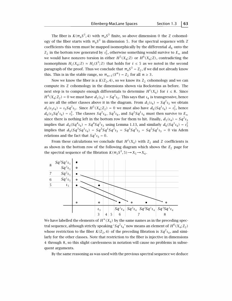
Eilenberg-MacLane Spaces Section 1.3 63
The fiber is K(π4S3,4) with π4S
3 finite, so above dimension 0 the Z cohomol-
ogy of the fiber starts with π4S3 in dimension 5. For the spectral sequence with Z
coefficients this term must be mapped isomorphically by the differential d6 onto the
Z2 in the bottom row generated by ι23 , otherwise something would survive to E∞ and
we would have nonzero torsion in either H5(X4;Z) or H6(X4;Z) , contradicting the
isomorphism Hi(X4;Z) ≈ Hi(S3;Z) that holds for i ≤ 5 as we noted in the second
paragraph of the proof. Thus we conclude that π4S3 = Z2 , if we did not already know
this. This is in the stable range, so πn+1(Sn) = Z2 for all n ≥ 3.
Now we know the fiber is a K(Z2,4) , so we know its Z2 cohomology and we can
compute its Z cohomology in the dimensions shown via Bocksteins as before. The
next step is to compute enough differentials to determine Hi(X4) for i ≤ 8. Since
H4(X4;Z2) = 0 we must have d5(ι4) = Sq2ι3 . This says that ι4 is transgressive, hence
so are all the other classes above it in the diagram. From d5(ι4) = Sq2ι3 we obtain
d5(ι3ι4) = ι3Sq2ι3 . Since H5(X4;Z2) = 0 we must also have d6(Sq1ι4) = ι23 , hence
d6(ι3Sq1ι4) = ι33 . The classes Sq2ι4 , Sq3ι4 , and Sq2Sq1ι4 must then survive to E∞
since there is nothing left in the bottom row for them to hit. Finally, d5(ι4) = Sq2ι3implies that d9(Sq
4ι4) = Sq4Sq2ι3 using Lemma 1.13, and similarly d6(Sq1ι4) = ι23
implies that d9(Sq3Sq1ι4) = Sq3Sq1Sq2ι3 = Sq3Sq3ι3 = Sq5Sq1ι3 = 0 via Adem
relations and the fact that Sq1ι3 = 0.
From these calculations we conclude that Hi(X4) with Z2 and Z coefficients is
as shown in the bottom row of the following diagram which shows the E2 page for
the spectral sequence of the fibration K(π5S3,5)→X5→X4 .
−−−−−−−−−−−−−−−−−−−−−−−−−−−−−−−−−−−−−−−−−−−−−−−−−−−→
−−−−−−−−−−−−−−−−−−−−−−−−−−−−−−−−−−−−−−−−−−−−−−−−−−−−−−−−−−−−−−−−−−−−−−−−−−−−−→
−−−−−−−−−−−−−−−−−−−−−−−−−−−−−−−−−−−−−−−−−−−−−−−−→
3 4 5
5
7
8
6
6 7 8ι3
ι5
ι42Sq ι43Sq ι41Sq3Sq
ι51Sq
ι51Sq2Sq
ι52Sqι53Sq
ι42Sq 1Sq
We have labelled the elements of H∗(X4) by the same names as in the preceding spec-
tral sequence, although strictly speaking ‘Sq2ι4 ’ now means an element of H6(X4;Z2)whose restriction to the fiber K(Z2,4) of the preceding fibration is Sq2ι4 , and simi-
larly for the other classes. Note that restriction to the fiber is injective in dimensions
4 through 8, so this slight carelessness in notation will cause no problems in subse-
quent arguments.
By the same reasoning as was used with the previous spectral sequence we deduce

64 Chapter 1 The Serre Spectral Sequence
that π5(S3) must be Z2 . Also we have the three nonzero differentials shown, d6(ι5) =
Sq2ι4 , d7(Sq1ι5) = Sq3ι4 , and d8(Sq
2ι5) = Sq2Sq2ι4 = Sq3Sq1ι4 . This is enough to
conclude that H7(X5;Z2) is Z2 with generator Sq2Sq1ι4 . By the universal coefficient
theorem this implies that H8(X5;Z) is cyclic (and of course finite). To determine its
order we look at the terms with p+q = 8 in the spectral sequence with Z coefficients.
In the fiber there is only the element Sq3ι5 . This survives to E∞ since d9(Sq3ι5) =
Sq3Sq2ι4 , and this is 0 by the Adem relation Sq3Sq2 = 0. The product ι3ι5 exists
only with Z2 coefficients. In the base there is only Sq3Sq1ι4 which survives to E∞with Z coefficients but not with Z2 coefficients. Thus H8(X5;Z) has order 4, and
since we have seen that it is cyclic, it must be Z4 .
Now we look at the spectral sequence for the next
fibration K(π6S3,6)→X6→X5 . With Z2 coefficients
the two differentials shown are isomorphisms as be-
fore. With Z coefficients the upper differential must
−−−−−−−−−−−−−−−−−−−−−−−−−−−−−−−−−−−−−−−−−−−−−−−−−−−→−−−−−−−−−−−−−−−−−−−−−−−−−−−−−−−−−−−−−−−−−−−−−−−→
3
67
7 8be an injection π6(S
3)→Z4 since H7(X6;Z) = 0, and
it must in fact be an isomorphism since after reducing
mod 2 this differential becomes an isomorphism via the Z2 coefficient information.
Recall that we are ignoring odd torsion, so in fact π6(S3) is Z12 rather than Z4 since
its odd torsion is Z3 . This finishes the theorem for S3 .
For S4 we can use the Hopf bundle S3→S7→S4 . The inclusion of the fiber into
the total space is nullhomotopic, and a nullhomotopy can be used to produce splitting
homomorphisms in the associated long exact sequence of homotopy groups, yielding
isomorphisms πi(S4) ≈ πi(S7)⊕πi−1(S
3) . Taking i = 5,6,7 then gives the theorem
for S4 . Note that the suspension map π5(S3)→π6(S
4) , which is guaranteed to be
surjective by the Freudenthal suspension theorem, is in fact an isomorphism since
both groups are Z2 .
For Sn with n ≥ 5 the groups πn+i(Sn) , i ≤ 3, are in the stable range, so
it remains only to compute the stable group πs3 , say π10(S7) . This requires only
minor changes in the spectral sequence arguments above. For the first fibration
K(π8S7,8)→X8→K(Z,7) we have the following diagram:

Eilenberg-MacLane Spaces Section 1.3 65
−−−−−−−−−−−−−−−−−−−−−−−−−−−−−−−−−−−−−−−−−−−−−−−−−−→
−−−−−−−−−−−−−−−−−−−−−−−−−−−−−−−−−−−−−−−−−−−−−−−−−−−−−−−−−−−−−−−−−−−−−−−−−−−−−−−−−→
−−−−−−−−−−−−−−−−−−−−−−−−−−−−−−−−−−−−−−−−−−−−−−−−−−−−−−−−−−−−−−−−−−−−−−−−−−−−−→
−−−−−−−−−−−−−−−−−−−−−−−−−−−−−−−−−−−−−−−−−−−−−−−−−−→
7 98
8
10
11
12
9
10 11 12 13ι7
ι8
ι72Sq ι73Sq ι72Sq4Sq
ι81Sq
ι81Sq2Sqι81Sq3Sq
ι82Sqι83Sq
ι84Sq
ι74Sq ι75Sq ι76Sq
There are no terms of interest off the two axes. The differentials can be computed
using Adem relations, starting with the fact that d9(ι8) = Sq2ι7 . Thus we have
d10(Sq1ι8) = Sq1Sq2ι7 = Sq3ι7
d11(Sq2ι8) = Sq2Sq2ι7 = Sq3Sq1ι7 = 0
d12(Sq3ι8) = Sq3Sq2ι7 = 0
d12(Sq2Sq1ι8) = Sq2Sq1Sq2ι7 = Sq2Sq3ι7 = Sq5ι7 + Sq4Sq1ι7 = Sq5ι7
d13(Sq3Sq1ι8) = Sq3Sq1Sq2ι7 = Sq3Sq3ι7 = Sq5Sq1ι7 = 0
d13(Sq4ι8) = Sq4Sq2ι7
With Z coefficients Sq5ι7 survives to E∞ , so we deduce that H12(X8;Z) has order 4
while H12(X8;Z2) = Z2 , hence H12(X8;Z) = Z4 . The generator of this Z4 corresponds
to Sq3Sq1ι8 while the element of order 2 corresponds to Sq5ι7 , in view of the way
that E∞ is related to the filtration of H∗(X8;Z) in the Serre spectral sequence for
cohomology. In other words, restriction to the fiber sends H12(X8;Z) = Z4 onto the
Z2 generated by Sq3Sq1ι8 , and the kernel of this restriction map is Z2 generated
by the image of Sq5ι7 ∈ H12(K(Z,7);Z) under the map induced by the projection
X8→K(Z,7) .For the next fibration K(π9S
7,9)→X9→X8 we have the picture below:
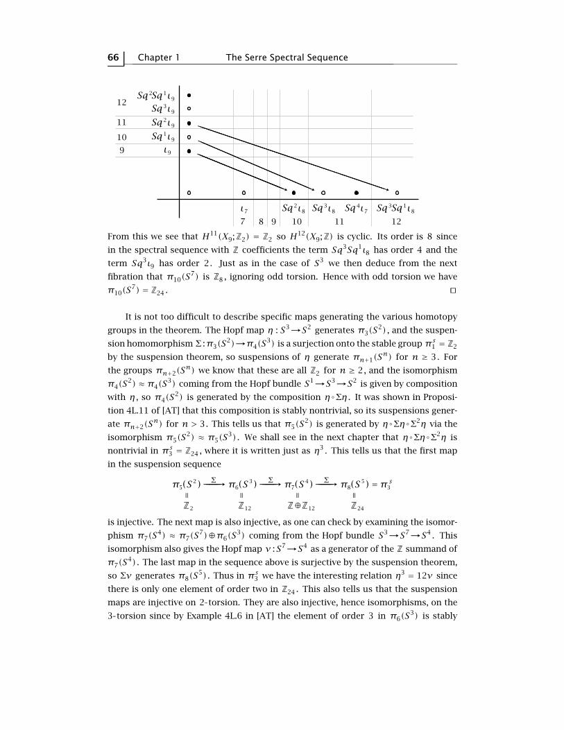
66 Chapter 1 The Serre Spectral Sequence
−−−−−−−−−−−−−−−−−−−−−−−−−−−−−−−−−−−−−−−−−−−−−−−−−−−→
−−−−−−−−−−−−−−−−−−−−−−−−−−−−−−−−−−−−−−−−−−−−−−−−−−−−−−−−−−−−−−−−−−−−−−−−−−−−−→
−−−−−−−−−−−−−−−−−−−−−−−−−−−−−−−−−−−−−−−−−−−−−−−−→
7 8 9
9
11
12
10
10 11 12ι7
ι9
ι82Sq ι83Sq ι81Sq3Sq
ι91Sq
ι91Sq2Sq
ι92Sqι93Sq
ι74Sq
From this we see that H11(X9;Z2) = Z2 so H12(X9;Z) is cyclic. Its order is 8 since
in the spectral sequence with Z coefficients the term Sq3Sq1ι8 has order 4 and the
term Sq3ι9 has order 2. Just as in the case of S3 we then deduce from the next
fibration that π10(S7) is Z8 , ignoring odd torsion. Hence with odd torsion we have
π10(S7) = Z24 . tu
It is not too difficult to describe specific maps generating the various homotopy
groups in the theorem. The Hopf map η : S3→S2 generates π3(S2) , and the suspen-
sion homomorphism Σ :π3(S2)→π4(S
3) is a surjection onto the stable group πs1 = Z2
by the suspension theorem, so suspensions of η generate πn+1(Sn) for n ≥ 3. For
the groups πn+2(Sn) we know that these are all Z2 for n ≥ 2, and the isomorphism
π4(S2) ≈ π4(S
3) coming from the Hopf bundle S1→S3→S2 is given by composition
with η , so π4(S2) is generated by the composition ηΣη . It was shown in Proposi-
tion 4L.11 of [AT] that this composition is stably nontrivial, so its suspensions gener-
ate πn+2(Sn) for n > 3. This tells us that π5(S
2) is generated by ηΣηΣ2η via the
isomorphism π5(S2) ≈ π5(S
3) . We shall see in the next chapter that ηΣηΣ2η is
nontrivial in πs3 = Z24 , where it is written just as η3 . This tells us that the first map
in the suspension sequence
−−−−−→S( )π5
2
2 −−−−−→S( )π63 −−−−−→S( )π7
4 S( )π8 π35 s=
Z
=
12Z
=
12ZZ
=
24Z
=
⊕
Σ Σ Σ
is injective. The next map is also injective, as one can check by examining the isomor-
phism π7(S4) ≈ π7(S
7)⊕π6(S3) coming from the Hopf bundle S3→S7→S4 . This
isomorphism also gives the Hopf map ν :S7→S4 as a generator of the Z summand of
π7(S4) . The last map in the sequence above is surjective by the suspension theorem,
so Σν generates π8(S5) . Thus in πs3 we have the interesting relation η3 = 12ν since
there is only one element of order two in Z24 . This also tells us that the suspension
maps are injective on 2 torsion. They are also injective, hence isomorphisms, on the
3 torsion since by Example 4L.6 in [AT] the element of order 3 in π6(S3) is stably

Eilenberg-MacLane Spaces Section 1.3 67
nontrivial, being detected by the Steenrod power P1 . The surjection Z⊕Z12→Z24 is
then the quotient map obtained by setting twice a generator of the Z summand equal
to a generator of the Z12 summand.
A generator for π6(S3) = Z12 can be constructed from the unit quaternion group
S3 as follows. The map S3×S3→S3 , (u,v), uvu−1v−1 , sends the wedge sum
S3×1∪1×S3 to 1, hence induces a quotient map S3∧S3→S3 , and this generates
π6(S3) , although we are not in a position to show this here.
The technique we have used here for computing homotopy groups of spheres
can be pushed considerably further, but eventually one encounters ambiguities which
cannot be resolved purely on formal grounds. In the next section we will study a more
systematic refinement of this procedure in the stable dimension range, the Adams
spectral sequence.
A Few References for Chapter 1
A. Borel, Sur la cohomologie des espaces fibres principaux et des espaces homogenes de
groups de Lie compacts, Ann. of Math. 57 (1953), 115–207.
P. Hilton, G. Mislin, and J. Roitberg, Localization of Nilpotent Groups and Spaces, North-
Holland, 1975.
S. MacLane, Homology, Springer-Verlag, 1963.
J. P. May, A general approach to Steenrod operations, Springer Lecture Notes 168 (1970), 153–
231.
J. McCleary, A User’s Guide to Spectral Sequences, second edition, Cambridge Univ. Press,
2001.
R. Mosher and M. Tangora, Cohomology Operations and Applications in Homotopy Theory,
Harper & Row, 1968.
D. Ravenel, Complex Cobordism and Stable Homotopy Groups of Spheres, Academic Press,
1986.
J.-P. Serre, Homologie singuliere des espaces fibres, Ann. of Math. 54 (1951), 425–505.
J.-P. Serre, Cohomologie modulo 2 des complexes d’Eilenberg-MacLane, Comment. Math. Helv.
27 (1953), 198–232.
D. Sullivan, Genetics of homotopy theory and the Adams conjecture, Ann. of Math. 100 (1974),
1–79.


![HOMOLOGICAL ALGEBRA AND THE EILENBERG-MOORE …HOMOLOGICAL ALGEBRA AND THE EILENBERG-MOORE SPECTRAL SEQUENCE BY LARRY SMITHO) In [6] Eilenberg and Moore have developed a spectral sequence](https://img.dokumen.tips/doc/110x75/5ed9532ff59b0f56f45f4725/homological-algebra-and-the-eilenberg-moore-homological-algebra-and-the-eilenberg-moore.jpg)