11 GENERAL CIRCULATION...330 CHAPTER 11 • GENERAL CIRCULATION 11.1. KEY TERMS Lines of constant latitude are called parallels, and winds parallel to the parallels are identified

329

Copyright © 2017 by Roland Stull. Practical Meteorology: An Algebra-based Survey of Atmospheric Science. v1.02

11 GENERAL CIRCULATION

A spatial imbalance between radiative inputs and outputs exists for the earth-ocean-atmosphere system. The earth loses energy at all latitudes due to outgoing infrared (IR) radiation. Near the trop-ics, more solar radiation enters than IR leaves, hence there is a net input of radiative energy. Near Earth’s poles, incoming solar radiation is too weak to totally offset the IR cooling, allowing a net loss of energy. The result is differential heating, creating warm equatorial air and cold polar air (Fig. 11.1a). This imbalance drives the global-scale general circulation of winds. Such a circulation is a fluid-dynamical analogy to Le Chatelier’s Principle of chemistry. Namely, an imbalanced system reacts in a way to partially counteract the imbalance. The continued destabilization by radiation causes a gen-eral circulation of winds that is unceasing. Because buoyancy causes warmer air to rise and colder air to sink, you might guess that equator-to-pole overturning would exist (Fig. 11.1b). Instead, the real general circulation has three bands of circu-lations in the Northern Hemisphere (Fig. 11.1c), and three in the Southern. In this chapter, we will iden-tify characteristics of the general circulation, explain why they exist, and learn how they work.

Contents

11.1. Key Terms 330

11.2. A Simple Description of the Global Circulation 33011.2.1. Near the Surface 33011.2.2. Upper-troposphere 33111.2.3. Vertical Circulations 33211.2.4. Monsoonal Circulations 333

11.3. Radiative Differential Heating 33411.3.1. North-South Temperature Gradient 33511.3.2. Global Radiation Budgets 33611.3.3. Radiative Forcing by Latitude Belt 33811.3.4. General Circulation Heat Transport 338

11.4. Pressure Profiles 34011.4.1. Non-hydrostatic Pressure Couplets 34011.4.2. Hydrostatic Thermal Circulations 341

11.5. Geostrophic Wind & Geostrophic Adjustment 34311.5.1. Ageostrophic Winds at the Equator 34311.5.2. Definitions 34311.5.3. Geostrophic Adjustment - Part 1 344

11.6. Thermal Wind Effect 34511.6.1. Definition of Thickness 34611.6.2. Thermal-wind Components 34611.6.3. Case Study 34811.6.4. Thermal Wind & Geostrophic Adj.-Part 2. 349

11.7. Explaining the General Circulation 35011.7.1. Low Latitudes 35011.7.2. High Latitudes 35211.7.3. Mid-latitudes 35211.7.4. Monsoon 356

11.8. Jet Streams 35711.8.1. Baroclinicity & the Polar Jet 35911.8.2. Angular Momentum & Subtropical Jet 360

11.9. Types of Vorticity 36211.9.1. Relative-vorticity Definition 36211.9.2. Absolute-vorticity Definition 36311.9.3. Potential-vorticity Definition 36311.9.4. Isentropic Potential Vorticity Definition 364

11.10. Horizontal Circulation 365

11.11. Extratropical Ridges & Troughs (Rossby Waves) 36711.11.1. Barotropic Instability 36711.11.2. Baroclinic Instability 37111.11.3. Meridional Transport by Rossby Waves 374

11.12. Three-band Global Circulation 37611.12.1. A Metric for Vertical Circulation 37711.12.2. Effective Vertical Circulation 377

11.13. Ekman Spiral of Ocean Currents 378

11.14. Review 379

11.15. Homework Exercises 380

“Practical Meteorology: An Algebra-based Survey of Atmospheric Science” by Roland Stull is licensed under a Creative Commons Attribution-NonCommercial-ShareAlike 4.0 International License. View this license at http://creativecommons.org/licenses/by-nc-sa/4.0/ . This work is available at https://www.eoas.ubc.ca/books/Practical_Meteorology/

Figure 11.1Radiative imbalances create (a) warm tropics and cold poles, in-ducing (b) buoyant circulations. Add Earth’s rotation, and (c) three circulation bands form in each hemisphere.

Earth image credit: NASA

cool

war

m

warm

(a)

cool

Hadley cell

Hadley cell

Rossby waves

Rossby waves

Polar cell

Polar cell(c) cool

warm warm

cool

(b) cool

war

m

warm

cool

330 CHAPTER11•GENERALCIRCULATION

11.1. KEY TERMS

Lines of constant latitude are called parallels, and winds parallel to the parallels are identified as zonal flows (Fig. 11.2). Lines of constant longitude are called meridians, and winds parallel to the me-ridians are known as meridional flows. Between latitudes of 30° and 60° are the mid-latitudes. High latitudes are 60° to 90°, and low latitudes are 0° to 30°. Each 1° of latitude = 111 km. Tropics, subtropics, subpolar, and polar re-gions are as shown in Fig. 11.2. Regions not in the tropics are called extratropical; namely, poleward of about 30°N and about 30°S. For example, tropical cyclones such as hur-ricanes are in the tropics. Low-pressure centers (lows, as indicated by L on weather maps) outside of the tropics are called extratropical cyclones. In many climate studies, data from the months of June, July, and August (JJA) are used to repre-sent conditions in N. Hemisphere summer (and S. Hemisphere winter). Similarly, December, January, February (DJF) data are used to represent N. Hemi-sphere winter (and S. Hemisphere summer).

11.2. A SIMPLIFIED DESCRIPTION OF THE GLOB-

AL CIRCULATION

This section summarizes “what” happens. The subsequent sections explain “why” and “how”. Consider a hypothetical rotating planet with no contrast between continents and oceans. The climatological average (average over 30 years; see the Climate chapter) winds in such a simpli-fied planet would have characteristics as sketched in Figs. 11.3. Actual winds on any day could dif-fer from this climatological average due to transient weather systems that perturb the average flow. Also, monthly-average conditions tend to shift toward the summer hemisphere (e.g., the circulation bands shift northward during April through September).

11.2.1. Near the Surface Near-surface average winds are sketched in Fig. 11.3a. At low latitudes are broad bands of persistent easterly winds (U ≈ –7 m s–1) called trade winds, named because the easterlies allowed sailing ships to conduct transoceanic trade in the old days. These trade winds also blow toward the equa-tor from both hemispheres, and the equatorial belt of convergence is called the intertropical conver-gence zone (ITCZ). On average, the air at the ITCZ

A SCIENTIFIC PERSPECTIVE • Idealiza-tions of Nature

Natural atmospheric phenomena often involve the superposition of many different physical processes and scales of motion. Large-scale average conditions are said to be caused by zeroth-order processes. Dominant variations about the mean are controlled by first-order processes. Finer details are caused by higher-order processes. Sometimes insight is possible by stripping away the higher-order processes and focusing on one or two lower orders. Equations that describe such sim-plified physics are known as toy models. With the right simplifications, some toy models admit analyti-cal solutions. Compare this to the unsimplified phys-ics, which might be too complicated to solve analyti-cally (although numerical solutions are possible). A rotating spherical “aqua planet” with no conti-nents and with uniform temperature is one example of a zeroth-order toy model. A first-order toy mod-el might add the north-south temperature variation, while neglecting east-west and continent-ocean vari-ations. With even more sophistication, seasonal or monthly variations might be explained. We will take the approach in this chapter to start with zeroth-order models to focus on basic climate concepts, and then gradually add more realism. John Harte (1988) wrote a book demonstrating the utility of such toy models. It is “Consider a Spherical Cow”, by University Science Books. 283 pages.

Figure 11.2Global key terms.

30°N

30°S

60°N

60°S

90°N

0°

latitude:

90°S

mer

idia

n

equator

midlatitudes

low latitudes

low latitudes

high latitudes

high latitudespolar

polar

tropical orequatorial

subtropical

subtropical

60°W

subpolar

subpolar

extratropical

extratropical

zonal flow

longitude =

90°W

30th parallel

north pole

south pole

midlatitudes

meri

dion

al f

low

R.STULL•PRACTICALMETEOROLOGY 331

is hot and humid, with low pressure, strong upward air motion, heavy convective (thunderstorm) pre-cipitation, and light to calm winds except in thun-derstorms. This equatorial trough (low-pressure belt) was called the doldrums by sailors whose sailing ships were becalmed there for many days. At 30° latitude are belts of high surface pressure called subtropical highs (Fig. 11.3a). In these belts are hot, dry, cloud-free air descending from higher in the troposphere. Surface winds in these belts are also calm on average. In the old days, becalmed sail-ing ships would often run short of drinking water, causing horses on board to die and be thrown over-board. Hence, sailors called these miserable places the horse latitudes. On land, many of the world’s deserts are near these latitudes. In mid-latitudes are transient centers of low pres-sure (mid-latitude cyclones, L) and high pressure (anticyclones, H). Winds around lows converge (come together) and circulate cyclonically — coun-terclockwise in the N. Hemisphere, and clockwise in the S. Hemisphere. Winds around highs diverge (spread out) and rotate anticyclonically — clock-wise in the N. Hemisphere, and counterclockwise in the S. Hemisphere. The cyclones are regions of bad weather (clouds, rain, high humidity, strong winds) and fronts. The anticyclones are regions of good weather (clear skies or fair-weather clouds, no pre-cipitation, dry air, and light winds). The high- and low-pressure centers move on av-erage from west to east, driven by large-scale winds from the west. Although these westerlies dominate the general circulation at mid-latitudes, the surface winds are quite variable in time and space due to the sum of the westerlies plus the transient circulations around the highs and lows. Near 60° latitude are belts of low surface pres-sure called subpolar lows. Along these belts are light to calm winds, upward air motion, clouds, cool temperatures, and precipitation (as snow in winter). Near each pole is a climatological region of high pressure called a polar high. In these regions are often clear skies, cold dry descending air, light winds, and little snowfall. Between each polar high (at 90°) and the subpolar low (at 60°) is a belt of weak easterly winds, called the polar easterlies.

11.2.2. Upper-troposphere The stratosphere is strongly statically stable, and acts like a lid to the troposphere. Thus, vertical circulations associated with our weather are most-ly trapped within the troposphere. These vertical circulations couple the average near-surface winds with the average upper-tropospheric (near the tro-popause) winds described here (Fig. 11.3b). In the tropics is a belt of very strong equatorial

Figure 11.3Simplified global circulation in the troposphere: (a) near the sur-face, and (b) near the tropopause. H and L indicate high and low pressures, and HHH means very strong high pressure. White indicates precipitating clouds. CAUTION: high and low pres-sures are RELATIVE to the average pressure AT THE SAME ALTITUDE. All absolute pressures near the tropopause are actually lower than the near-surface pressures.

a) Near Surface

Polar High

Polar High

60°N

30°N

0°

30°S

60°S

L L L

H

H

Trade Winds

L L L L

Trade Winds

North-Easterlies

South-Easterlies

H H H HSubtropical Highs

Subpolar Lows

L L LSubpolar Lows

H H H HSubtropical Highs

ITCZdoldrums calm

Westerlies

Westerlies

L

L

H

H

b) Near Tropopause

troug

h

trough

rid

ge

ridge

Polar Low

Polar Low

HH HH HH HHSubtropical Jet

HH HH HH HHSubtropical Jet

60°N

30°N

0°

30°S

60°S

L

L

HHH HHH HHH HHH

Polar Jet

Polar Jet


high pressure along the tops of the ITCZ thunder-storms. Air in this belt blows from the east, due to easterly inertia from the trade winds being carried upward in the thunderstorm convection. Diverging from this belt are winds that blow toward the north in the N. Hemisphere, and toward the south in the S. Hemisphere. As these winds move away from the equator, they turn to have an increasingly westerly component as they approach 30° latitude. Near 30° latitude in each hemisphere is a persis-tent belt of strong westerly winds at the tropopause called the subtropical jet. This jet meanders north and south a bit. Pressure here is very high, but not as high as over the equator. In mid-latitudes at the tropopause is another belt of strong westerly winds called the polar jet. The centerline of the polar jet meanders north and south, resulting in a wave-like shape called a Rossby wave (or planetary wave), as sketched in Fig. 11.1c. The equatorward portions of the wave are known as low-pressure troughs, and poleward portions are known as high-pressure ridges. These ridges and troughs are very transient, and generally shift from west to east relative to the ground. Near 60° at the tropopause is a belt of low to me-dium pressure. At each pole is a low-pressure cen-ter near the tropopause, with winds at high latitudes generally blowing from the west causing a cyclonic circulation around the polar low. Thus, contrary to near-surface conditions, the near-tropopause av-erage winds blow from the west at all latitudes (ex-cept near the equator).

11.2.3. Vertical Circulations Vertical circulations of warm rising air in the tropics and descending air in the subtropics are called Hadley cells or Hadley circulations (Fig. 11.4). At the bottom of the Hadley cell are the trade winds. At the top, near the tropopause, are diver-gent winds. The updraft portion of the Hadley cir-culation often contains thunderstorms and heavy precipitation at the ITCZ. This vigorous convection in the troposphere causes a high tropopause (15 - 18 km altitude) and a belt of heavy rain in the tropics. The summer- and winter-hemisphere Hadley cells are strongly asymmetric (Fig. 11.4). The major Hadley circulation (denoted with subscript “M”) crosses the equator, with rising air in the sum-mer hemisphere and descending air in the winter hemisphere. The updraft is often between 0° and

Figure 11.4 (at left)Vertical cross section of Earth’s global circulation in the tropo-sphere. (a) N. Hemisphere summer. (b) Transition months. (c) S. Hemisphere summer. The major (subscript M) Hadley cell is colored in red and blue. Minor circulations have no subscript.

Polar Cell | Ferrel Cell | Hadley C

ell | Hadley C

ell M | Ferrel Cell M

| Polar Cell

0°

30°

60°

–30°

–60°

90°

–90°

ITCZ

a) June, July, August,September

15°sunlightSummer

Hemisphere

WinterHemisphere

Polar | Ferrel | Hadley | H

adley | Ferrel | Polar

0°

30°

60°

–30°

–60°

90°

–90°

ITCZb) April, May

& October,November

14.9°sunlight

Polar Cell | Ferrel Cell M | Hadley C

ell M | H

adley Cell | Ferrel Cell | Polar Cell

0°

30°

60°

–30°

–60°

90°

–90°

ITCZ

c) December,January, February,

March

SummerHemisphere

WinterHemisphere


15° latitudes in the summer hemisphere, and has average core vertical velocities of 6 mm s–1. The broader downdraft is often found between 10° and 30° latitudes in the winter hemisphere, with average velocity of about –4 mm s–1 in downdraft centers. Connecting the up- and downdrafts are meridional wind components of 3 m s–1 at the cell top & bottom. The major Hadley cell changes direction and shifts position between summer and winter. During June-July-August-September, the average solar dec-lination angle is 15°N, and the updraft is in the Northern Hemisphere (Fig. 11.4a). Out of these four months, the most well-defined circulation occurs in August and September. At this time, the ITCZ is centered at about 9°N, but varies with longitude. During December-January-February-March, the average solar declination angle is 14.9°S, and the major updraft is in the Southern Hemisphere (Fig. 11.4c). Out of these four months, the strongest circu-lation is during February and March, and the ITCZ is centered at roughly 6°S, but varies with longitude. The major Hadley cell transports significant heat away from the tropics, and also from the summer to the winter hemisphere. During the transition months (April-May and October-November) between summer and winter, the Hadley circulation has nearly symmetric Hadley cells in both hemispheres (Fig. 11.4b). During this transition, the intensities of the Hadley circulations are weak. When averaged over the whole year, the strong but reversing major Hadley circulation partially cancels itself, resulting in an annual average circula-tion that is somewhat weak and looks like Fig. 11.4b. This weak annual average is deceiving, and does not reflect the true movement of heat, moisture, and momentum by the winds. Hence, climate experts prefer to look at months JJA and DJF separately to give seasonal averages. In the winter hemisphere, one or more jet streams circle the earth at mid-latitudes while meandering north and south as Rossby waves (Fig. 11.1c). When averaged around latitude bands, the net effect is a weak vertical circulation called a Ferrel cell. At high latitudes is a modest polar cell. In the summer hemisphere, all the circulations are weaker. There are minor Hadley and Ferrel cells (Fig. 11.4). Summer-hemisphere circulations are weaker because the temperature contrast between the tropics and poles are weaker.

11.2.4. Monsoonal Circulations Monsoon circulations are continental-scale circulations driven by continent-ocean tempera-ture contrasts, as sketched in Figs. 11.5. In summer, high-pressure centers (anticyclones) are over the

Figure 11.5Idealized seasonal-average monsoon circulations near the sur-face. Continents are shaded dark brown; oceans are light green. H and L are surface high- and low-pressure centers.

a) June, July, August

HL L

H HL

summer

winter

North Pole

South Pole

b) December, January, February

H H

HL L

L

summer

winter

North Pole

South Pole


relatively warm oceans, and low-pressure centers (cyclones) are over the hotter continents. In winter, low-pressure centers are over the cool oceans, and high-pressure centers are over the colder continents. These monsoon circulations represent average conditions over a season. The actual weather on any given day can be variable, and can deviate from these seasonal averages. Our Earth has a complex arrangement of conti-nents and oceans. As a result, seasonally-varying monsoonal circulations are superimposed on the seasonally-varying planetary-scale circulation to yield a complex and varying global-circulation pat-tern.

At this point, you have a descriptive understand-ing of the global circulation. But what drives it?

11.3. RADIATIVE DIFFERENTIAL HEATING

The general circulation is driven by differential heating. Incoming solar radiation (insolation) nearly balances the outgoing infrared (IR) radiation when averaged over the whole globe. However, at different latitudes are significant imbalances (Fig. 11.6), which cause the differential heating. Recall from the Solar & Infrared Radiation chap-ter that the flux of solar radiation incident on the top of the atmosphere depends more or less on the cosine of the latitude, as shown in Fig. 11.7. The component of the incident ray of sunlight that is perpendicular to the Earth’s surface is small in polar regions, but larger toward the equator (grey dashed arrows in Figs. 11.6 and 11.7). The incoming energy adds heat to the Earth-atmosphere-ocean system. Heat is lost due to infrared (IR) radiation emitted from the Earth-ocean-atmosphere system to space. Since all locations near the surface in the Earth-ocean-atmosphere system are relatively warm com-pared to absolute zero, the Stefan-Boltzmann law from the Solar & Infrared Radiation chapter tells us that the emission rates are also more or less uni-form around the Earth. This is sketched by the solid black arrows in Fig. 11.6. Thus, at low latitudes, more solar radiation is ab-sorbed than leaves as IR, causing net warming. At high latitudes, the opposite is true: IR radiative loss-es exceed solar heating, causing net cooling. This differential heating drives the global circulation. The general circulation can’t instantly eliminate all the global north-south temperature differences. What remains is a meridional temperature gradient — the focus of the next subsection.

Figure 11.7Of the solar radiation approaching the Earth (thick solid yellow arrows), the component (dashed grey arrow) that is perpendic-ular to the top of the atmosphere is proportional to the cosine of the latitude ϕ (during the equinox).

Figure 11.6Annual average incoming solar radiation (yellow dashed arrows) and outgoing infrared (IR) radiation (solid dark red arrows), where arrow length indicates relative magnitude. [Because the Earth rotates and exposes all locations to the sun at one time or another during the year, the incoming solar radiation is sketched as approaching all locations on the Earth’s surface.]

OutgoingIR Radiation

IncomingSolar

RadiationEarth

Earth

solar radiation

solar radiation

NP

equator

ϕ

ϕ


11.3.1. North-South Temperature Gradient To create a first-order toy model, neglect month-ly variations, monsoonal variations and mountains. Instead, focus on surface temperatures averaged around separate latitude belts and over one year. Those latitude belts near the equator are warmer, and those near the poles are colder (Fig. 11.8a). One equation that roughly approximates the variation of zonally-averaged surface temperature T with lati-tude ϕ is:

T a b≈ + +

· cos · ·sin3 2132

φ φ (11.1)

where a ≈ –12°C is an offset and b ≈ 40°C is a tem-perature difference between equator and pole. The equation above applies only to the surface. At higher altitudes the north-south temperature dif-ference is smaller, and even becomes negative in the stratosphere (i.e., warm over the poles and cold over the tropics). To account for this altitude variation, b cannot be a constant. Instead, use:

b bz

zT≈ −

1 1· (11.2)

where average tropospheric depth is zT ≈ 11 km, pa-rameter b1 = 40°C, and z is height above the surface. A similarly crude but useful generalization of parameter a can be made so that it too changes with altitude z above sea level:

a ≈ a1 – γ · z (11.3)

where a1 = –12°C and γ = 3.14 °C km–1. In Fig. 11.8a, the temperature curve looks like a flattened cosine wave. The flattened curve indicates somewhat uniformly warm temperatures between ±30° latitude, caused the strong mixing and heat transport by the Hadley circulations. With uniform tropical temperatures, the remain-ing change to colder temperature is pushed to the mid-latitude belts. The slope of the Fig. 11.8a curve is plotted in Fig. 11.8b. This slope is the north-south (meridional) temperature gradient:

∆∆

≈ −Ty

b c· ·cos ·sin2 3φ φ (11.4)

where y is distance in the north-south direction, c = 1.18x10–3 km–1 is a constant valid at all heights, and b is given by eq. (11.2) which causes the gradient to change sign at higher altitudes (e.g., at z = 15 km). Because the meridional temperature gradient results from the interplay of differential radiative heating and advection by the global circulation, let us now look at radiative forcings in more detail.

Sample Application What is the value of annual zonal average tempera-ture and meridional temperature gradient at 50°S lati-tude for the surface and for z = 15 km.

Find the AnswerGiven: ϕ = –50°, (a) z = 0 (surface), and (b) z = 15 kmFind: Tsfc = ? °C, ∆T/∆y = ? °C km–1

a) z = 0. Apply eq. (11.2): b = (40°C)·(1–0) = 40°C.Apply eq. (11.3): a = (–12°C)–0°C = –12°C. Apply eq. (11.1) : T C Co ≈ − + − + −12 40 50 1

32

503 2° °( )· cos ( · ·sin (°) °)

= 7.97 °C

Apply eq. (11.4):∆∆

≈ − × − −−Ty

C( )·( . )·cos ( ·sin (40 1 18 10 50 53 2 3° °) 00°) =0.0087°C km–1

b) z = 15 km.Apply eq. (11.2): b = (40°C)·[1–(15/11)] = –14.55°C.Apply (11.3): a = (–12°C)–(3.14°C/km)·(15km) = –59.1°C.Apply eq. (11.1) :T C Ckm15

3 259 1 14 6 50 132

≈ − − − + −. . · cos ( · ·sin (° ° °) 550°)

=–66.4°C

Apply eq. (11.4) at z = 15 km:∆∆

≈ + × −−Ty

C( . )·( . )·cos ( ·sin14 55 1 18 10 503 2 3° °) ((−50°) =–0.0032 °C km–1

Check: Phys. & units reasonable. Agrees with Fig. 11.8 for Southern Hemisphere.Exposition: Cold at z = 15 km even though warm at z = 0. Gradient signs would be opposite in N. Hem.

Figure 11.8Idealized variation of annual-average temperature (a) and meridional temperature gradient (b) with latitude, averaged around latitude belts (i.e., zonal averages). Solid curve repre-sents Earth’s surface (= sea-level because the toy model neglects terrain) and dotted curve is for 15 km altitude above sea level.

–20 0 20–90

–60

–30

0

30

60

90

Latit

ude

(°)

-0.01 0 0.01

(a) (b)N

S

∆T / ∆y (°C/km)T (°C)

Equator


11.3.2. Global Radiation Budgets

11.3.2.1. Incoming Solar Radiation Because of the tilt of the Earth’s axis and the change of seasons, the actual flux of incoming solar radiation is not as simple as was sketched in Fig. 11.6. But this complication was already discussed in the Solar & Infrared Radiation chapter, where we saw an equation to calculate the incoming solar radiation (insolation) as a function of latitude and day. The resulting insolation figure is reproduced below (Fig. 11.9a). If you take the spreadsheet data from the Solar & Infrared Radiation chapter that was used to make this figure, and average rows of data (i.e., average over all months for any one latitude), you can find the annual average insolation Einsol for each latitude (Fig. 11.9b). Insolation in polar regions is not small. The curve in Fig. 11.9b is simple, and in the spirit of a toy model can be nicely approximated by:

Einsol = Eo + E1 · cos(2 ϕ) (11.5)

where the empirical parameters are Eo = 298 W m–2, E1 = 123 W m–2, and ϕ is latitude. This curve and the data points it approximates are plotted in Fig. 11.10. But not all the radiation incident on the top of the atmosphere is absorbed by the Earth-ocean-at-mosphere system. Some is reflected back into space from snow and ice on the surface, from the oceans, and from light-colored land. Some is reflected from cloud top. Some is scattered off of air molecules.

HIGHER MATH • Derivation of the North-South Temperature Gradient

The goal is to find ∂T/∂y for the toy model.

a) First, expand the derivative: ∂∂

= ∂∂

∂∂

Ty

Tyφφ

· (a)

We will look at factors ∂T/∂ϕ and ∂ϕ/∂y separately:

b) Factor ∂ϕ/∂y describes the meridional gradient of latitude. Consider a circumference of the Earth that passes through both poles. The total latitude change around this circle is ∆ϕ = 2π radians. The total cir-cumference of this circle is ∆y = 2πR for average Earth radius of R = 6371 km. Hence:

∂∂

= = =φ φ ππy y R R

∆∆ ·

22

1 (b)

c) For factor ∂T/∂ϕ, start with eq. (11.1) for the toy model: T a b≈ + +

· cos · ·sin3 2132

φ φ (11.1)

and take its derivative vs. latitude: ∂∂

=

Tb

φ· ·

32

2 323

3 2 2sin ·cos cos sin cos · sinφ φ φ φ φ φ( ) − +

Next, take the common term (sinϕ · cos2ϕ) out of [ ]:

∂∂

=

− −

T

bφ

φ φ φ φ32

2 2 32 2 2sin ·cos · cos sin

Use the trig. identity: cos2ϕ = 1 – sin2ϕ. Hence: 2 cos2ϕ = 2 – 2 sin2ϕ . Substituting this in into the previous full-line equation gives:

∂∂

=

−

Tb

φφ φ φ3

252 2sin ·cos · sin (c)

d) Plug equations (b) and (c) back into eq. (a):

∂∂

= −

Ty

bR

· · ·sin ·cos152

1 3 2φ φ (d)

Define: c

R=

=

= × −15

21 15

21

63711 177 10 3· · .

kmkkm 1−

Thus, the final answer is:

∆∆

· ·sin ·cosTy

Ty

b c≈ ∂∂

= − 3 2φ φ (11.4)

Check: Fig. 11.8 shows the curves that were calcu-lated from eqs. (11.1) and (11.4). The fact that the sign and shape of the curve for ∆T/∆y is consistent with the curve for T(y) suggests the answer is reasonable.

Alert: Eqs. (11.4) and (11.1) are based on a highly ide-alized “toy model” of the real atmosphere. They were designed only to illustrate first-order effects.

Figure 11.9(a) Solar radiation (W m–2) incident on the top of the atmo-sphere for different latitudes and months (copied from the Solar & Infrared Radiation chapter). The slight asymmetry about the equator is because Earth’s orbit is closer to the sun during S. Hemisphere summer. (b) Meridional variation of insolation, found by averaging the data from the left figure over all months for each separate latitude (i.e., averages for each row of data).

(a) (b)

0 100 200 300

Relative Julian Day

Latit

ude

(°)

–90

–60

–30

0

30

60

90Jan Mar May Jul Sep NovFeb Apr Jun Aug Oct Dec

100 100

100

0

00

200200

200

300300

300

400400 W/m2

400

500

500500

0 200 400Avg. Insolation

(W/m2)

AnnualAverage


The amount of insolation that is NOT absorbed is surprisingly constant with latitude at about E2 ≈ 110 W m–2. Thus, the amount that IS absorbed is:

Ein = Einsol – E2 (11.6)

where Ein is the incoming flux (W m–2) of solar ra-diation absorbed into the Earth-ocean-atmosphere system (Fig. 11.10). This absorbed radiation causes heating.

11.3.2.2. Outgoing Terrestrial Radiation As you learned in the Satellites & Radar chap-ter, infrared radiation emission and absorption in the atmosphere are very complex. At some wave-lengths the atmosphere is mostly transparent, while at others it is mostly opaque. Thus, some of the IR emissions to space are from the Earth’s surface, some from cloud top, and some from air at middle altitudes in the atmosphere. In the spirit of a toy model, suppose that the net IR emissions are characteristic of the absolute tem-perature Tm near the middle of the troposphere (at about zm = 5.5 km). Approximate the outbound flux of radiation Eout (averaged over a year and averaged around latitude belts) by the Stefan-Boltzmann law (see the Solar & Infrared Radiation chapter):

E Tout SB m≈ ε σ· · 4 (11.7)

where the effective emissivity is ε ≈ 0.9 (see the Cli-mate chapter), and the Stefan-Boltzmann constant is σSB = 5.67x10–8 W·m–2·K–4. When you use z = zm = 5.5 km in eqs. (11.1 - 11.3) to get Tm vs. latitude for use in eq. (11.7), the result is Eout vs. ϕ, as plotted in Fig. 11.10.

11.3.2.3. Net Radiation For an air column over any square meter of the Earth’s surface, the radiative input minus output gives the net radiative flux:

E E Enet in out= − (11.8)

which is plotted in Fig. 11.10 for our toy model.

Sample Application Estimate the annual average solar energy absorbed at the latitude of the Eiffel Tower in Paris, France.

Find the AnswerGiven: ϕ = 48.8590° (at the Eiffel tower)Find: Ein = ? W m–2

Use eq. (11.5): Einsol = (298 W m–2) + (123 W m–2)·cos(2 · 48.8590°) = (298 W m–2) – (16.5 W m–2) = 281.5 W m–2 Use eq. (11.6): Ein = 281.5 W m–2 – 110.0 W m–2 = 171.5 W m–2

Check: Units OK. Agrees with Fig. 11.10.Exposition: The actual annual average Ein at the Ei-ffel Tower would probably differ from this zonal avg.

Sample Application. What is Enet at the Eiffel Tower latitude?Find the Answer. Given: ϕ = 48.8590°, z = 5.5 km, Ein = 171.5 W m–2 from previous Sample Application Find: Enet = ? W m–2 Apply eq. (11.2): b = (40°C)·[ 1 – (5.5 km/11 km)] = 20°C Apply eq.(11.3): a=(-12°C)–(3.14°C km–1)·(5.5 km) = -29.27°C Apply eq. (11.1): Tm = –18.73 °C = 254.5 K Apply eq.(11.7): Eout=(0.9)·(5.67x10–8W·m–2·K–4)·(254.5 K)4 = 213.8 W m–2 Apply eq. (11.8): Enet = (171.5 W m–2) – (213.8 W m–2) = –42.3 W m–2 Check: Units OK. Agrees with Fig. 11.10Exposition: The net radiative heat loss at Paris latitude must be compensated by winds blowing heat in.

Figure 11.10Data points are insolation vs. latitude from Fig. 11.9b. Eq. 11.5 approximates this insolation Einsol (thick black line). Ein is the solar radiation that is absorbed (thin solid line, from eq. 11.6). Eout is outgoing terrestrial (IR) radiation (dashed; from eq. 11.7). Net flux Enet = Ein – Eout. Positive Enet causes heating; negative causes cooling.

-200

-100

0

100

200

300

400

500

-90 -60 -30 0 30 60 90

Latitude (°)

Enet

Flu

x (W

/m2 )

Einsol

Ein

Eout

NS


11.3.3. Radiative Forcing by Latitude Belt Do you notice anything unreasonable about Enet in Fig. 11.10? It appears that the negative area un-der the curve is much greater than the positive area, which would cause the Earth to get colder and cold-er — an effect that is not observed. Don’t despair. Eq. (11.8) is correct, but we must remember that the circumference [2π·REarth·cos(ϕ)] of a parallel (a constant latitude circle) is smaller near the poles than near the equator. ϕ is latitude and the average Earth radius REarth is 6371 km. The solution is to multiply eqs. (11.6 - 11.8) by the circumference of a parallel. The result

E R EEarthφ φ= π2 · ·cos( )· (11.9)

can be applied for E = Ein, or E = Eout, or E = Enet. This converts from E in units of W m–2 to Eϕ in units of W m–1, where the distance is north-south distance. You can interpret Eϕ as the power being transferred to/from a one-meter-wide sidewalk that encircles the Earth along a parallel. Figs. (11.11) and (11.12) show the resulting incom-ing, outgoing, and net radiative forcings vs. latitude. At most latitudes there is nonzero net radiation. We can define Enet as differential heating Dϕ :

D E E Enet in outφ φ φ φ= = − (11.10)

Our despair is now quelled, because the surplus and deficit areas in Figs. 11.11 and 11.12 are almost ex-actly equal in magnitude to each other. Hence, we anticipate that Earth’s climate should be relatively steady (neglecting global warming for now).

11.3.4. General Circulation Heat Transport Nonetheless, the imbalance of net radiation be-tween equator and poles in Fig. 11.12 drives atmo-spheric and oceanic circulations. These circulations act to undo the imbalance by removing the excess heat from the equator and depositing it near the poles (as per Le Chatelier’s Principle). First, we can use the radiative differential heating to find how much global-circulation heat transport is needed. Then, we can examine the actual heat transport by atmospheric and oceanic circulations.

11.3.4.1. The Amount of Transport Required Meridional transport at each pole is zero, be-cause the pole is a singularity where all meridians converge. If we sum Dϕ from Fig. 11.12 over all lati-tude belts from the North Pole to any other latitude ϕ , we can find the total transport Tr required for the global circulation to compensate all the radiative imbalances north of that latitude:

Sample Application From the previous Sample Application, find the zonally-integrated differential heating at ϕ = 48.859°.

Find the AnswerGiven: Enet = –42.3 W m–2 , ϕ = 48.859° at Eiffel TowerFind: Dϕ = ? GW m–1

Combine eqs. (11.8-11.10): Dϕ = 2π·REarth·cos(ϕ)·Enet = 2(3.14159)·(6.357x106m)·cos(48.859°)·(–42.3 W m–2) = –1.11x109 W m–1 = –1.11 GW m–1

Check: Units OK. Agrees with Fig. 11.12.Exposition: Net radiative heat loss at this latitude is compensated by warm Gulf stream and warm winds.

Figure 11.11Zonally-integrated radiative forcings for absorbed incoming solar radiation (solid line) and emitted net outgoing terrestrial (IR) radiation (dashed line). The surplus balances the deficit.

0

5

10

-90 -60 -30 0 30 60 90

In

Out| Eϕ |

(GW/m)

Latitude (°) NS

Surplus

Defici

t Deficit

Figure 11.12Net (incoming minus outgoing) zonally-integrated radiative forcings on the Earth. Surplus balances deficits. This differen-tial heating imposed on the Earth must be compensated by heat transport by the global circulation; otherwise, the tropics would keep getting hotter and the polar regions colder.

-1

0

1

2

-90 -60 -30 0 30 60 90

Dϕ

(GW/m)

Latitude (°)NS

Surplus

DeficitDeficit

heattransport

heattransport


Tr D yo

( ) ( )·φ φφ

φ= − ∆

=∑

90° (11.11)

where the width of any latitude belt is ∆y. [Meridional distance ∆y is related to latitude change ∆ϕ by: ∆y(km) = (111 km/°) · ∆ϕ (°) .] The resulting “needed transport” is shown in Fig. 11.13, based on the simple “toy model” tempera-ture and radiation curves of the past few sections. The magnitude of this curve peaks at about 5.6 PW (1 petawatt equals 1015 W) at latitudes of about 35° North and South (positive Tr means northward transport).

11.3.4.2. Transport Achieved Satellite observations of radiation to and from the Earth, estimates of heat fluxes to/from the ocean based on satellite observations of sea-surface tem-perature, and in-situ measurements of the atmo-sphere provide some of the transport data needed. Numerical forecast models are then used to tie the observations together and fill in the missing pieces. The resulting estimate of heat transport achieved by the atmosphere and ocean is plotted in Fig. 11.14. Ocean currents dominate the total heat transport only at latitudes 0 to 17°, and remain important up to latitudes of ± 40°. Asymmetry of the ocean curve across the equator is due to the different ocean basin shapes and currents. In the atmosphere, the Hadley circulation is a dominant contributor in the tropics and subtropics, while the Rossby waves dominate atmospheric transport at mid-latitudes. Knowing that global circulations undo the heat-ing imbalance raises another question. How does the differential heating in the atmosphere drive the winds in those circulations? That is the subject of the next three sections.

Sample Application What total heat transports by the atmosphere and ocean circulations are needed at 50°N latitude to com-pensate for all the net radiative cooling between that latitude and the North Pole? The differential heating as a function of latitude is given in the following table (based on the toy model):

Lat (°) Dϕ (GW m–1)

Lat (°) Dϕ (GW m–1)

90 0 65 –1.38085 –0.396 60 –1.40380 –0.755 55 –1.33175 –1.049 50 –1.16470 –1.261 45 –0.905

Find the AnswerGiven: ϕ = 50°N. Dϕ data in table above.Find: Tr = ? PW

Use eq. (11.11). Use sidewalks (latitude belts) each of width ∆ϕ = 5°. Thus, ∆y (m) = (111,000 m/°) · (5°) = 555,000 m is the sidewalk width. If one sidewalk spans 85 - 90°, and the next spans 80 - 85° etc, then the values in the table above give Dϕ along the edges of the side-walk, not along the middle. A better approximation is to average the Dϕ values from each edge to get a value representative of the whole sidewalk. Using a bit of algebra, this works out to:Tr = – (555000 m)· [(0.5)·0.0 – 0.396 – 0.755 – 1.049 – 1.261 – 1.38 – 1.403 – 1.331 – (0.5)·1.164] (GW m–1)Tr = (555000 m)·[8.157 GW m–1] = 4.527 PW

Check: Units OK (106 GW = 1 PW). Agrees with Fig. 11.14. Exposition: This northward heat transport warms all latitudes north of 50°N, not just one side-walk. The warming per sidewalk is ∆Tr/∆ϕ .

Figure 11.13Required heat transport Tr by the global circulation to com-pensate radiative differential heating, based on a simple “toy model”. Agrees very well with actual achieved transport in Fig. 11.14.

–90S

–60 –30 0 30 60 90N

Latitude (°)

Tr

(PW)

6

4

2

0

–2

–4

–6

total

total

Figure 11.14Meridional heat transports: Satellite-observed total (solid line) & ocean estimates (dotted). Atmospheric (dashed) is found as a residual. 1 PW = 1 petaWatt = 1015 W. [Data from K. E. Tren-berth and J. M. Caron, 2001: “J. Climate”, 14, 3433-3443.]

–90S

–60 –30 0 30 60 90N

Latitude (°)

Tr

(PW)

6

4

2

0

–2

–4

–6

total

total

atmos-phere

atmos-phere

ocean

ocean


11.4. PRESSURE PROFILES

The following fundamental concepts can help you understand how the global circulation works: •non-hydrostaticpressurecoupletscausedby horizontal winds and vertical buoyancy, •hydrostaticthermalcirculations, •geostrophicadjustment,and •thethermalwind.The first two concepts are discussed in this section. The last two are discussed in subsequent sections.

11.4.1. Non-hydrostatic Pressure Couplets Consider a background reference environment with no vertical acceleration (i.e., hydrostatic). Namely, the pressure-decrease with height causes an upward pressure-gradient force that exactly bal-ances the downward pull of gravity, causing zero net vertical force on the air (see Fig. 1.12 and eq. 1.25). Next, suppose that immersed in this environment is a column of air that might experience a different pressure decrease (Fig. 11.15); i.e., non-hydrostatic pressures. At any height, let p’ = Pcolumn – Phydrostatic be the deviation of the actual pressure in the column from the theoretical hydrostatic pressure in the en-vironment. Often a positive p’ in one part of the atmospheric column is associated with negative p’ elsewhere. Taken together, the positive and nega-tive p’s form a pressure couplet. Non-hydrostatic p’ profiles are often associated with non-hydrostatic vertical motions through Newton’s second law. These non-hydrostatic mo-tions can be driven by horizontal convergence and divergence, or by buoyancy (a vertical force). These two effects create opposite pressure couplets, even though both can be associated with upward motion, as explained next.

11.4.1.1. Horizontal Convergence/Divergence If external forcings cause air near the ground to converge horizontally, then air molecules accumu-late. As density ρ increases according to eq. (10.60), the ideal gas law tells us that p’ will also become positive (Fig. 11.16a). Non-zero p’ implies that a pres-sure gradient exists, which will drive winds. Positive p’ does two things: it (1) decelerates the air that was converging horizontally, and (2) acceler-ates air vertically in the column. Thus, the pressure perturbation causes mass continuity (horizontal inflow near the ground balances vertical outflow). Similarly, an externally imposed horizontal di-vergence at the top of the troposphere would lower the air density and cause negative p’, which would also accelerate air in the column upward. Hence, we

A SCIENTIFIC PERSPECTIVE • Residuals

If something you cannot measure contributes to things you can measure, then you can estimate the unknown as the residual (i.e., difference) from all the knowns. This is a valid scientific approach. It was used in Fig. 11.14 to estimate the atmospheric portion of global heat transport. CAUTION: When using this approach, your re-sidual not only includes the desired signal, but it also includes the sums of all the errors from the items you measured. These errors can easily accumulate to cause a “noise” that is larger than the signal you are trying to estimate. For this reason, error esti-mation and error propagation (see Appendix A) should always be done when using the method of residuals.

Figure 11.15Background hydrostatic pressure (solid line), and non-hydro-static column of air (dashed line) with pressure perturbation p’ that deviates from the hydrostatic pressure Phydrostatic at most heights z. In this example, even though p’ is positive (+) near the tropopause, the total pressure in the column (Pcolumn = Phy-

drostatic + p’) at the tropopause is still less than the surface pres-sure. The same curve is plotted as (a) linear and as (b) semilog.

100604020000

5

10

15

20

P ( kPa )

z (

km ) tropopause

near-surface

(a)p´= +

100105 20 50

0

5

10

15

20

P ( kPa )

z (

km ) tropopause

near-surface

(b)p´= +

p´= –

p´= –


expect upward motion (W = positive) to be driven by a p’ couplet, as shown in Fig. 11.16a.

11.4.1.2. Buoyant Forcings For a different scenario, suppose air in a column is positively buoyant, such as in a thunderstorm where water-vapor condensation releases lots of latent heat. This vertical buoyant force creates up-ward motion (i.e., warm air rises, as in Fig. 11.16b). As air in the thunderstorm column moves away from the ground, it removes air molecules and low-ers the density and the pressure; hence, p’ is negative near the ground. This suction under the updraft causes air near the ground to horizontally converge, thereby conserving mass. Conversely, at the top of the troposphere where the thunderstorm updraft encounters the even warmer environmental air in the stratosphere, the upward motion rapidly decelerates, causing air mol-ecules to accumulate, making p’ positive. This pres-sure perturbation drives air to diverge horizontally near the tropopause, causing the outflow in the an-vil-shaped tops of thunderstorms. The resulting pressure-perturbation p’ couplet in Fig. 11.16b is opposite that in Fig. 11.16a, yet both are associated with upward vertical motion. The reason for this pressure-couplet difference is the difference in driving mechanism: imposed horizontal conver-gence/divergence vs. imposed vertical buoyancy.

Similar arguments can be made for downward motions. For either upward or downward motions, the pressure couplets that form depend on the type of forcing. We will use this process to help explain the pressure patterns at the top and bottom of the troposphere.

11.4.2. Hydrostatic Thermal Circulations Cold columns of air tend to have high surface pressures, while warm columns have low surface pressures. Figs. 11.17 illustrate how this happens. Consider initial conditions (Fig. 11.17i) of two equal columns of air at the same temperature and with the same number of air molecules in each col-umn. Since pressure is related to the mass of air above, this means that both columns A and B have the same initial pressure (100 kPa) at the surface. Next, suppose that some process heats one col-umn relative to the other (Fig. 11.17ii). Perhaps con-densation in a thunderstorm cloud causes latent heating of column B, or infrared radiation cools col-umn A. After both columns have finished expand-ing or contracting due to the temperature change, they will reach new hydrostatic equilibria for their respective temperatures.

Figure 11.16(a) Vertical motions driven by pressure gradients caused by hor-izontal convergence or divergence. (b) Vertical motions driven by buoyancy. In both figures, black arrows indicate the cause (the driving force), and white arrows are the effect (the response). p’ is the pressure perturbation (deviation from hydrostatic), and thin dashed lines are isobars of p’. U and W are horizontal and vertical velocities. In both figures, the responding flow (white arrows) is driven down the pressure-perturbation gradient, away from positive p’ and toward negative p’.

p´= +

p´= –

x

z

tropo-pause

near-surface

(a) W driven by horizontal convergence/div.

U U

UU

W

p´= –

p´= +

x

z

tropo-pause

near-surface

(b) W driven by buoyancy

U U

UU

W


gain as many air molecules as they lose; hence, they are in mass equilibrium. This equilibrium circulation also transports heat. Air from the warm air column mixes into the cold column, and vice versa. This intermixing reduces the temperature contrast between the two columns, causing the corresponding equilibrium circulations to weaken. Continued destabilization (more latent heating or radiative cooling) would be needed to maintain the circulation.

The circulations and mass exchange described above can be realized at the equator. At other lati-tudes, the exchange of mass is often slower (near the surface) or incomplete (aloft) because Coriolis force turns the winds to some angle away from the pres-sure-gradient direction. This added complication, due to geostrophic wind and geostrophic adjust-ment, is described next.

The hypsometric equation (see Chapter 1) says that pressure decreases more rapidly with height in cold air than in warm air. Thus, although both col-umns have the same surface pressure because they contain the same number of molecules, the higher you go above the surface, the greater is the pres-sure difference between warm and cold air. In Fig. 11.17ii, the printed size of the “H” and “L” indicate the relative magnitudes of the high- and low-pres-sure perturbations p’. The horizontal pressure gradient ∆P/∆y aloft be-tween the warm and cold air columns drives hori-zontal winds from high toward low pressure (Fig. 11.17iii). Since winds are the movement of air mol-ecules, this means that molecules leave the regions of high pressure-perturbation and accumulate in the regions of low. Namely, they leave the warm column, and move into the cold column. Since there are now more molecules (i.e., more mass) in the cold column, it means that the surface pressure must be greater (H) in the cold column (Fig. 11.17iv). Similarly, mass lost from the warm column results in lower (L) surface pressure. This is called a thermal low. A result (Fig. 11.17iv) is that, near the surface, high pressure in the cold air drives winds toward the low pressure in warm air. Aloft, high pressure-perturbation in the warm air drives winds towards low pressure-perturbation in the cold air. The re-sulting thermal circulation causes each column to

Figure 11.17Formation of a thermal circulation. The response of two columns of air that are heated differently is that the warmer air column de-velops a low pressure perturbation at the surface and a high pressure perturbation aloft. Response of the cold column is the opposite. Notation: H = high pressure perturbation (i.e., relative to the average pressure at that altitude). L = low pressure perturbation (relative to the average pressure at that same altitude). Black dots represents air parcels. Thin arrows are winds (i.e., movement of air parcels).

100

50

10

100

50

10

100

5040

30

20

A B

100

50

Acolder

Bwarmer

90

5040

30

10

100110

50

10

20

30

Acolder

Bwarmer

100

5040

30

100

50

2030

Acolder

Bwarmer

(i) Initial Conditions (ii) (iii) (iv)

altertemper-atures

∆P/∆ydrives upper-

air winds

∆P/∆y also drives low-altitude winds

massredistrib-

utes

10

203040

10

10

10

P (

kPa)

y y yH L


11.5. GEOSTROPHIC WIND & GEOSTROPHIC AD-

JUSTMENT

11.5.1. Ageostrophic Winds at the Equator Air at the equator can move directly from high (H) to low (L) pressure (Fig. 11.18 - center part) un-der the influence of pressure-gradient force. Zero Coriolis force at the equator implies infinite geos-trophic winds. But actual winds have finite speed, and are thus ageostrophic (not geostrophic). Because such flows can happen very easily and quickly, equatorial air tends to quickly flow out of highs into lows, causing the pressure centers to neu-tralize each other. Indeed, weather maps at the equa-tor show very little pressure variations zonally. One exception is at continent-ocean boundaries, where continental-scale differential heating can continual-ly regenerate pressure gradients to compensate the pressure-equalizing action of the wind. Thus, very small pressure gradients can cause continental-scale (5000 km) monsoon circulations near the equator. Tropical forecasters focus on winds, not pressure. If the large-scale pressure is uniform in the hori-zontal near the equator (away from monsoon circu-lations), then the horizontal pressure gradients dis-appear. With no horizontal pressure-gradient force, no large-scale winds can be driven there. However, winds can exist at the equator due to inertia — if the winds were first created geostrophically at nonzero latitude and then coast across the equator. But at most other places on Earth, Coriolis force deflects the air and causes the wind to approach geostrophic or gradient values (see the Forces & Winds chapter). Non-accelerating geostrophic and gradient winds do not cross isobars, so they cannot transfer mass from highs to lows. Thus, significant pressure patterns (e.g., strong high and low centers, Fig. 11.18) can be maintained for long periods at mid-latitudes in the global circulation.

11.5.2. Definitions A temperature field is a map showing how tem-peratures are spatially distributed. A wind field is a map showing how winds are distributed. A mass field represents how air mass is spatially distribut-ed. But we don’t routinely measure air mass. In the first Chapter, we saw how pressure at any one altitude depends on (is a measure of) all the air mass above that altitude. So we can use the pres-sure field at a fixed altitude as a surrogate for the mass field. Similarly, the height field on a map of constant pressure is another surrogate. But the temperature and mass fields are cou-pled via the hypsometric equation (see Chapter 1).

A SCIENTIFIC PERSPECTIVE • The Scientific Method Revisited

“Like other exploratory processes, [the scientific method] can be resolved into a dialogue between fact and fancy, the actual and the possible; between what could be true and what is in fact the case. The pur-pose of scientific enquiry is not to compile an inven-tory of factual information, nor to build up a totali-tarian world picture of Natural Laws in which every event that is not compulsory is forbidden. We should think of it rather as a logically articulated structure of justifiable beliefs about a Possible World — a story which we invent and criticize and modify as we go along, so that it ends by being, as nearly as we can make it, a story about real life.”

- by Nobel Laureate Sir Peter Medawar (1982) Pluto’s Republic. Oxford Univ. Press.

Figure 11.18At the equator, winds flow directly from high (H) to low (L) pressure centers. At other latitudes, Coriolis force causes the winds to circulate around highs and lows. Smaller size font for H and L at the equator indicate weaker pressure gradients at that latitude.

H L

H L

H L

0°

30°N

30°S

60°N

60°S

90°N

90°S


Namely, if the temperature changes in the horizon-tal (defined as a baroclinic atmosphere), then pres-sures at any fixed altitude must also change in the horizontal. Later in this chapter, we will also see how the wind and temperature fields are coupled (via the thermal wind relationship).

11.5.3. Geostrophic Adjustment - Part 1 The tendency of non-equatorial winds to ap-proach geostrophic values (or gradient values for curved isobars) is a very strong process in the Earth’s atmosphere. If the actual winds are not in geostrophic balance with the pressure patterns, then both the winds and the pressure patterns tend to change to bring the winds back to geostrophic (another example of Le Chatelier’s Principle). Geo-strophic adjustment is the name for this process. Picture a wind field (grey arrows in Fig. 11.19a) initially in geostrophic equilibrium (Mo = Go) at alti-tude 2 km above sea level (thus, no drag at ground). We will focus on just one of those arrows (the black arrow in the center), but all the wind vectors will march together, performing the same maneuvers. Next, suppose an external process increases the horizontal pressure gradient to the value shown in Fig. 11.19b, with the associated faster theoretical geo-strophic wind speed G1. Inertia prevents instanta-neous response of the actual wind M. During this transition, pressure-gradient force FPG is greater than Coriolis force FCF. This force imbalance turns the wind M1 slightly toward low pressure and accel-erates the air (Fig. 11.19b). The component of wind M1 from high to low pressure horizontally moves air molecules, weaken-ing the pressure field and thereby reducing the theo-retical geostrophic wind (G2 in Fig. 11.19c). Namely, the wind field changed the mass (i.e., pressure) field. Simultaneously the actual wind accelerates to M2. Thus, the mass field also changed the wind field. After both fields have adjusted, the result is M2 > Mo and G2 < G1, with M2 = G2. These changes are called geostrophic adjustments. Define a “disturbance” as the region that was initially forced out of equilibrium. As you move further away from the disturbance, the amount of geostrophic adjustment diminished. The e-folding distance for this reduction is

λRBV T

c

N Zf

=·

•(11.12)

where λR is known as the internal Rossby defor-mation radius. The Coriolis parameter is fc, tropo-spheric depth is ZT, and the Brunt-Väisälä frequency is NBV (see eq. on page 372). λR is roughly 1300 km. For a given wavelength λ of the initial distur-bance, eq. (11.12) can be used as follows. For large

Sample Application Find the internal Rossby radius of deformation in a standard atmosphere at 45°N.

Find the AnswerGiven: ϕ = 45°. Standard atmosphere from Chapter 1: T(z = ZT =11 km) = –56.5°C, T(z=0) = 15°C.Find: λR = ? km

First, find fc = (1.458x10–4 s–1)·sin(45°) = 1.031x10–4 s–1 Next, find the average temperature and tempera-ture difference across the depth of the troposphere: Tavg = 0.5·(–56.5 + 15.0)°C = –20.8°C = 252 K ∆T = (–56.5 – 15.0) °C = –71.5°C across ∆z = 11 km (continued on next page)

Figure 11.19Example of geostrophic adjustment in the N. Hemisphere (not at equator). (a) Initial conditions, with the actual wind M (thick black arrow) in equilibrium with (equal to) the theoretical geos-trophic value G (white arrow with black outline). (b) Transition. (c) End result at a new equilibrium. Dashed lines indicate forces F. Each frame focuses on the region of disturbance. Note that both the wind AND the pressure gradient have adjusted.

y

x

G1

(b)

250 km

L

H

FPG

FCF

FPG

FCF

M1

y

x

(c)

250 km

L

H

FPG

FCF

M2

P = 79.6 kPa

P = 80.4 kPa

y

x

Go

(a)

250 km

L

H

FPG

FCF

Mo

G2 G1Go

P = 79.4 kPa

P = 80.6 kPa

P = 79.5 kPa

P = 80.5 kPa


disturbances (λ > λR), the wind field experiences the greatest adjustment. For smaller λ, the pressure and temperature fields have the greatest adjustment.

11.6. THERMAL WIND EFFECT

Recall that horizontal temperature gradients cause vertically varying horizontal pressure gradi-ents (Fig. 11.17), and that horizontal pressure gra-dients drive geostrophic winds. We can combine those concepts to see how horizontal temperature gradients drive vertically varying geostrophic winds. This is called the thermal wind effect. This effect can be pictured via the slopes of iso-baric surfaces (Fig. 11.20). The hypsometric equation from Chapter 1 describes how there is greater thick-ness between any two isobaric (constant pressure) surfaces in warm air than in cold air. This causes the tilt of the isobaric surfaces to change with alti-tude. But as described by eq. (10.29), tilting isobaric surface imply a pressure-gradient force that can drive the geostrophic wind (Ug, Vg). The relationship between the horizontal tem-perature gradient and the changing geostrophic wind with altitude is known as the thermal wind effect. After a bit of manipulation (see the Higher Math box on the next page), one finds that:

∆∆

≈− ∆

∆U

z

g

T fTy

g

v c

v·

· •(11.13a)

∆∆

≈∆∆

V

z

g

T fTx

g

v c

v·

· •(11.13b)

where the Coriolis parameter is fc, virtual absolute temperature is Tv, and gravitational acceleration magnitude is |g| = 9.8 m·s–2. Thus, the meridional temperature gradient causes the zonal geostrophic winds to change with altitude, and the zonal tem-perature gradient causes the meridional geostrophic winds to change with altitude. Above the atmospheric boundary layer, actual winds are nearly equal to geostrophic or gradient winds. Thus, eqs. (11.13) provide a first-order esti-mate of the variation of actual winds with altitude.

Sample Application While driving north a distance of 500 km, your car thermometer shows the outside air temperature de-creasing from 20°C to 10°C. How does the theoretical geostrophic wind change with altitude?

Find the AnswerGiven: ∆y = 500 km, ∆T = 10°C – 20°C = –10°C, average T = 0.5·(10+20°C) = 15°C = 288 K.Find: ∆Ug/∆z = ? (m s–1)/kmGiven lack of other data, for simplicity assume: fc = 10–4 s–1, and Tv = T (i.e., air is dry). Apply eq. (11.13a):

∆∆

≈ − −− −

U

zg ( . )

( )·( )·

( )(

9 8

288 10

10504

m/s

K s

C2

1°

00km) = 6.81 (m s–1)/km

Check: Physics & units reasonable. Agrees with Fig.Exposition: Even if the wind were zero at the ground, the answer indicates that a west wind will increase in speed by 6.81 m s–1 for each 1 km of altitude gained. Given no info about temperature change in the x direction, assume uniform temperature, which im-plies ∆Vg/∆z = 0 from eq. (11.13b). Namely, the south wind is constant with altitude.

Sample Application (continuation) Find the Brunt-Väisälä frequency (see the Atmos. Stability chapter). NBV = − +

( . ) ..

9 8252

71 511000

0 0098m/s

KKm

Km

== −0 0113 1. s

where the temperature differences in square brackets can be expressed in either °C or Kelvin. Finally, use eq. (11.12): λR = (0.0113 s–1)·(11 km) / (1.031x10–4 s–1) = 1206 km

Check: Physics, units & magnitude are reasonable.Exposition: When a cold-front over the Pacific approaches the steep mountains of western Canada, the front feels the influence of the mountains 1200 to 1300 km before reaching the coast, and begins to slow down.

Figure 11.20Isobaric surfaces are shaded brown. A zonal (west-east) tem-perature gradient causes the isobaric surfaces to tilt more and more with increasing altitude. Greater tilt causes stronger geo-strophic winds (Vg) meridionally (south-north), as plotted with the black vectors for the N. Hemisphere. Geostrophic winds are reversed in S. Hemisphere.

cool

coolP1=80

P2=70kPacoolcool

warm∆ z1

x

z

P0=90 Vg = 0

Vg

Vg

thickness

∆x

∆z2

∆xwarm

warmwarm

P3=60kPa

Vg warmwarm


11.6.1. Definition of Thickness In Fig. 11.20, focus on two isobaric surfaces, such as P = 90 kPa (dark brown in that figure), and P = 80 kPa (medium brown). These two surfaces are at different altitudes z, and the altitude difference is called the “thickness”. For our example, we focused on the “90 to 80 kPa thickness”. For any two isobaric surfaces P1 and P2 having altitudes z

P1 and z

P2 , the

thickness is defined as

TH = zP2

– zP1 •(11.14)

The hypsometric equation from Chapter 1 tells us that the thickness is proportional to the average ab-solute virtual-temperature within that layer. Colder air has thinner thickness. Thus, horizontal changes in temperature must cause horizontal changes in thickness. Weather maps of “100 to 50 kPa thickness” such as Fig. 11.21 are often created by forecast centers. Larger thickness on this map indicates warmer air within the lowest 5 km of the atmosphere.

11.6.2. Thermal-wind Components Suppose that we use thickness TH as a surrogate for absolute virtual temperature. Then we can com-bine eqs. (11.14) and (10.29) to yield:

U U Ug

fTHyTH G G

c= − = −2 1

∆∆ •(11.15a)

V V Vg

fTHxTH G G

c= − = +2 1

∆∆

•(11.15b)

HIGHER MATH • Thermal Wind Effect

Problem: Derive Thermal Wind eq. (11.13a).

Find the Answer: Start with the definitions of geostrophic wind (10.26a) and hydrostatic balance (1.25b):

U

fPy

gPzg

c= − ∂

∂= − ∂

∂1

ρρ

··and

Replace the density in both eqs using the ideal gas law (1.20). Thus:

U f

T PPy

g

T PPz

g c

v

d

v

d·= −

ℜ ∂∂

= −ℜ ∂

∂and

Use (1/P)·∂P = ∂ln(P) from calculus to rewrite both:

U f

TP

y

g

TP

zg c

vd

vd

· ln( ) ln( )= −ℜ ∂∂

= −ℜ ∂∂

and

Differentiate the left eq. with respect to z:

∂∂

= −ℜ ∂

∂ ∂z

U f

TP

y zg c

vd

· ln( )

and the right eq. with respect to y:

∂∂

= −ℜ ∂

∂ ∂y

g

TP

y zvd

ln( )

But the right side of both eqs are identical, thus we can equate the left sides to each other:

∂∂

= ∂∂

z

U f

T y

g

Tg c

v v

·

Next, do the indicated differentiations, and rearrange to get the exact relationship for thermal wind:

∂∂

= −∂∂

+∂∂

U

z

g

T fTy

U

TTz

g

v c

v g

v

v·

The last term depends on the geostrophic wind speed and the lapse rate, and has magnitude of 0 to 30% of the first term on the right. If we neglect the last term, we get the approximate thermal wind relationship:

∂∂

≈ −∂∂

U

z

g

T fTy

g

v c

v·

(11.13a)

Exposition: A barotropic atmosphere is when the geostrophic wind does not vary with height. Using the exact equation above, we see that this is possible only when the two terms on the right balance.

Figure 11.21Thickness chart based on a US National Weather Service 24-hour forecast. The surface cyclone center is at the “X”.

PacificOcean

Canada

Gulf ofMexico

AtlanticOcean

Mexico

X

5.1

5.2

5.3

5.4

5.5

5.6

5.7

Thin (cold)

Thick (warm)

100 to 50 kPa Thickness (km) 12 UTC, 23 Feb 1994


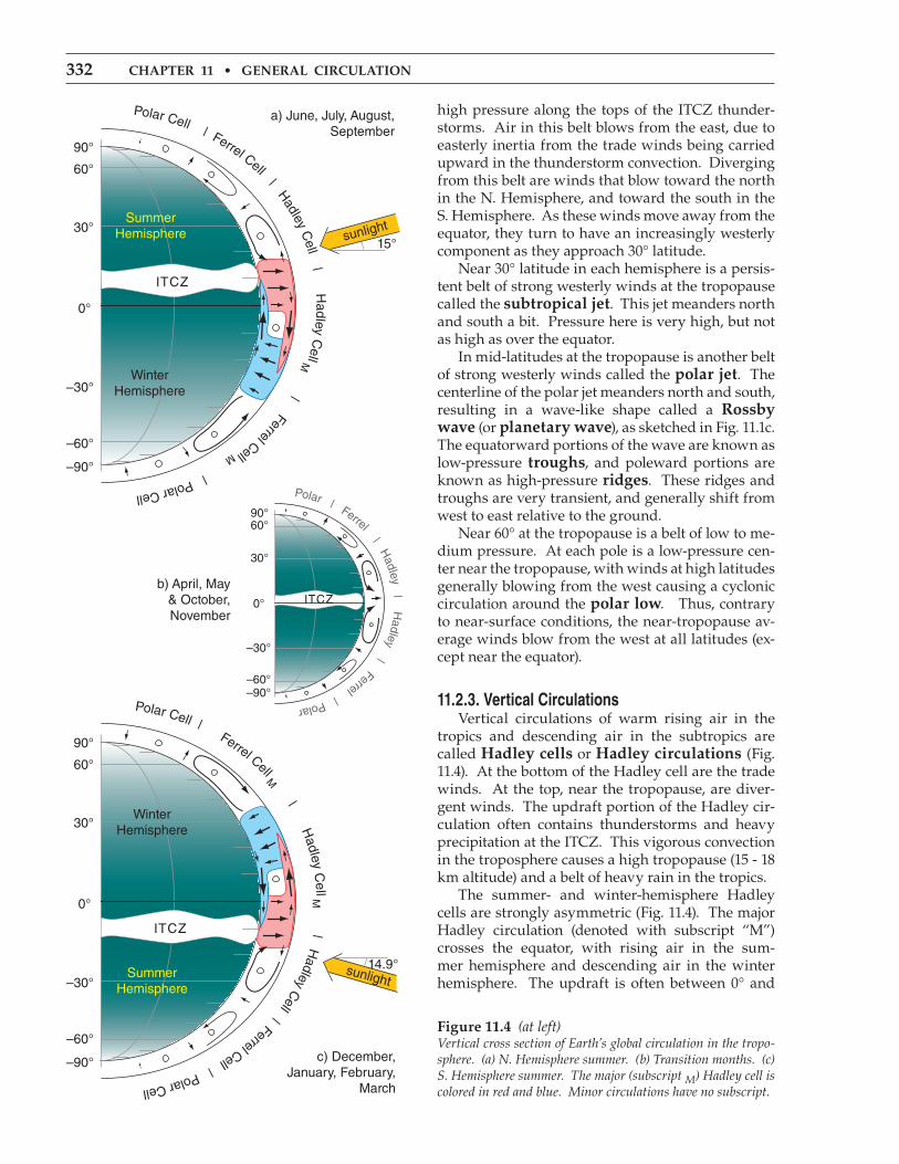
where UTH and VTH are components of the ther-mal wind, |g| = magnitude of gravitational-ac-celeration, fc = Coriolis parameter, (UG1, VG1) are geostrophic-wind components on the P1 isobaric surface, and (UG2, VG2) are geostrophic-wind com-ponents on the P2 isobaric surface. The horizontal vector defined by (UTH, VTH) is the difference between the geostrophic wind vector on the P2 surface and the geostrophic wind vector on the P1 surface, as Fig. 11.22 demonstrates. The corresponding magnitude of the thermal wind MTH is:

M U VTH TH TH= +2 2 (11.16)

To illustrate this, consider two isobaric surfaces P2 = 50 kPa (shaded blue in Figure 11.22) and P1 = 100 kPa (shaded red). The P1 surface has higher height to the east (toward the back of this sketch). If you conceptually roll a ball bearing down this red surface to find the direction of the pressure gradi-ent, and then recall that the geostrophic wind in the N. Hemisphere is 90° to the right of that direction, then you would anticipate a geostrophic wind G1 direction as shown by the red arrow. Namely, it is parallel to a constant height contour (dotted red line) pointing in a direction such that low heights are to the vector’s left. Suppose cold air in the north (left side of this sketch) causes a small thickness of only 4 km be-tween the red and blue surfaces. Warm air to the south causes a larger thickness of 5 km between the two isobaric surfaces. Adding those thicknesses to the heights of the P1 surface (red) give the heights of the P2 surface (blue). The blue P2 surface tilts more steeply than the red P1 surface, hence the geostroph-ic wind G2 is faster (blue arrow) and is parallel to a constant height contour (blue dotted line). Projecting the G1 and G2 vectors to the ground (green in Fig. 11.22), the vector difference is shown in yellow, and is labeled as the thermal wind MTH. It is parallel to the contours of thickness (i.e., perpen-dicular to the temperature gradient between cold and warm air) pointing in a direction with cold air (thin thicknesses) to its left (Fig. 11.23).

Sample Application. For Fig. 11.22, what are the thermal-wind components. Assume fc = 1.1x10–4 s–1.

Find the Answer. Given: TH2 = 4 km, TH1 = 5 km, ∆y = 1000 km from the figure, fc = 1.1x10–4 s–1.Find: UTH = ? m s–1, VTH = ? m s–1

Apply eq. (11.15a): Ug

fTHyTH

c=−

=− −×

−

− −∆∆

( . )·( )

( .

9 8 4 5

1 1 10 4ms km

s

2

11 km)·( )5000 = 17.8 m s–1

Check: Physics & units are reasonable. Positive sign for UTH indicates wind toward positive x direction, as in Fig.Exposition: With no east-to-west temperature gradient, and hence no east-to-west thickness gradient, we would expect zero north-south thermal wind;, hence, VTH = 0.

Figure 11.22Relationship between the thermal wind MTH and the geostroph-ic winds G on isobaric surfaces P. View is from the west north-west, in the Northern Hemisphere.

5

WARM

x

y

M TH

CO

LD

5

5

4

6

z(km)

1 1

2

3

4

6

7

0P 1 = 100 kPa

5

P 2 = 50 kPa

G1

G2

1000 km

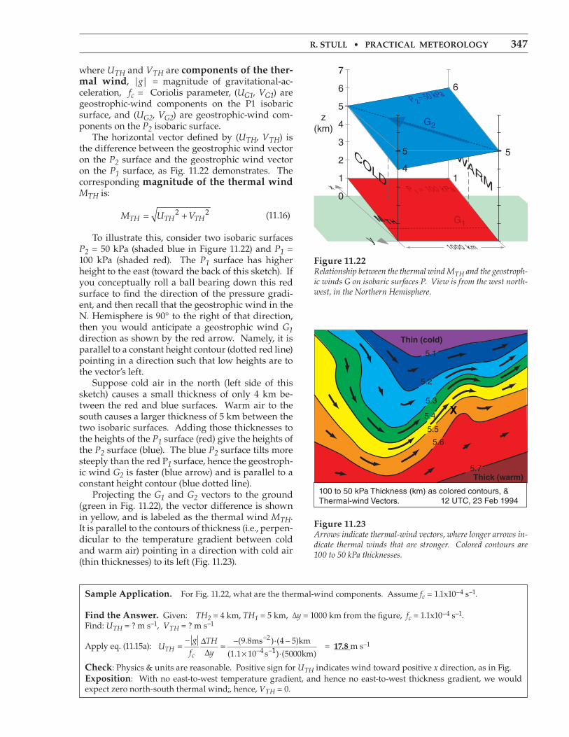
Figure 11.23Arrows indicate thermal-wind vectors, where longer arrows in-dicate thermal winds that are stronger. Colored contours are 100 to 50 kPa thicknesses.

PacificOcean

Canada

Gulf ofMexico

AtlanticOcean

Mexico

X

5.1

5.2

5.3

5.4

5.5

5.6

5.7

Thin (cold)

Thick (warm)

100 to 50 kPa Thickness (km) as colored contours, &Thermal-wind Vectors. 12 UTC, 23 Feb 1994


Thermal-wind magnitude is stronger where the thickness gradient is greater. Thus, regions on a weather map (Fig. 11.23) where thickness contours are closer together (i.e., have tighter packing) indi-cates faster thermal winds. The relationship between thermal winds and thickness contours is analogous to the relationship between geostrophic winds and height contours. But never forget that no physically realistic wind can equal the thermal wind, because the thermal wind represents the difference or shear between two geostrophic winds. Nonetheless, you will find the thermal-wind concept useful because it helps you anticipate how geostrophic wind will change with altitude. Actual winds tend towards being geostrophic above the at-mospheric boundary layer, hence the thermal-wind concept allows you to anticipate real wind shears.

11.6.3. Case Study Figs. 11.24 show how geostrophic winds and thermal winds can be found on weather maps, and how to interpret the results. These maps may be copied onto transparencies and overlain. Fig. 11.24a is a weather map of pressure at sea level in the N. Hemisphere, at a location over the northeast Pacific Ocean. As usual, L and H indicate low- and high-pressure centers. At point A, we can qualitatively draw an arrow (grey) showing the the-oretical geostrophic (G1) wind direction; namely, it is parallel to the isobars with low pressure to its left. Recall that pressures on a constant height surface (such as at height z = 0 at sea level) are closely related to geopotential heights on a constant pressure sur-face. So we can be confident that a map of 100 kPa heights would look very similar to Fig. 11.24a. Fig. 11.24b shows the 100 - 50 kPa thickness map, valid at the same time and place. The thickness be-tween the 100 and the 50 kPa isobaric surfaces is about 5.6 km in the warm air, and only 5.4 km in the cold air. The white arrow qualitatively shows the thermal wind MTH, as being parallel to the thick-ness lines with cold temperatures to its left. Fig. 11.24c is a weather map of geopotential heights of the 50 kPa isobaric surface. L and H in-dicate low and high heights. The black arrow at A shows the geostrophic wind (G2), drawn parallel to the height contours with low heights to its left. If we wished, we could have calculated quantita-tive values for G1, G2, and MTH, utilizing the scale that 5° of latitude equals 555 km. [ALERT: This scale does not apply to longitude, because the meridians get closer together as they approach the poles. However, once you have determined the scale (map mm : real km) based on latitude, you can use it to good approximation in any direction on the map.]

Figure 11.24Weather maps for a thermal-wind case-study. (a) Mean sea-level pressure (kPa), as a surrogate for height of the 100 kPa surface. (b) Thickness (km) of the layer between 100 kPa to 50 kPa isobaric surfaces. (c) Geopotential heights (km) of the 50 kPa isobaric surface.

35°N

55°N

50°N

45°N

40°N

160°W 150°W 140°W 130°W

A

BL

H

5.80

5.76

5.72

5.72

5.68

5.68

5.64

5.64

5.60

5.60

5.56

5.56

5.52

5.52

5.48

(c) z50kPa (km)7 UTC 28 May 2007

G2

35°N

55°N

50°N

45°N

40°N

160°W 150°W 140°W 130°W

A

BL99.3

H102.7

99.6100.0

100.4

100.8

101.2

101.2

101.6

101.6

102.0

102.4

102.4

(a) PMSL (kPa)7 UTC 28 May 2007

G1

35°N

55°N

50°N

45°N

40°N

160°W 150°W 140°W 130°W

A

B

Warm

Cold

Cool

5.45

5.40

5.505.50

5.55

5.55

5.60

5.60

(b) TH100-50kPa (km)7 UTC 28 May 2007

MTH


Back to the thermal wind: if you add the geos-trophic vector from Fig. 11.24a with the thermal wind vector from Fig. 11.24b, the result should equal the geostrophic wind vector in Fig. 11.24c. This is shown in the Sample Application. Although we will study much more about weath-er maps and fronts in the next few chapters, I will interpret these maps for you now. Point A on the maps is near a cold front. From the thickness chart, we see cold air west and north-west of point A. Also, knowing that winds rotate counterclockwise around lows in the N. Hemisphere (see Fig. 11.24a), I can anticipate that the cool air will advance toward point A. Hence, this is a region of cold-air advection. Associated with this cold-air advection is backing of the wind (i.e., turning counterclockwise with increasing height), which we saw was fully explained by the thermal wind. Point B is near a warm front. I inferred this from the weather maps because warmer air is south of point B (see the thickness chart) and that the coun-terclockwise winds around lows are causing this warm air to advance toward point B. Warm air advection is associated with veering of the wind (i.e., turning clockwise with increasing height), again as given by the thermal wind relationship. I will leave it to you to draw the vectors at point B to prove this to yourself.

11.6.4. Thermal Wind & Geostrophic Adjustment -

Part 2 As geostrophic winds adjust to changes in pres-sure gradients, they move mass to alter the pressure gradients. Eventually, an equilibrium is approached (Fig. 11.25) based on the combined effects of geos-trophic adjustment and the thermal wind. This fig-ure is much more realistic than Fig. 11.17(iv) because Coriolis force prevents the winds from flowing di-rectly from high to low pressure.

With these concepts of: •differentialheating, •nonhydrostaticpressurecoupletsdueto horizontal winds and vertical buoyancy, •hydrostaticthermalcirculations, •geostrophicadjustment,and •thethermalwind,we can now go back and explain why the global cir-culation works the way it does.

Sample Application For Fig. 11.24, qualitatively verify that when vector MTH is added to vector G1, the result is vector G2.

Find the AnswerGiven: the arrows from Fig. 11.24 for point A. These are copied and pasted here.Find: The vector sum of G1 + MTH = ?

Recall that to do a vector sum, move the tail of the second vector (MTH) to be at the arrow head of the first vector (G1). The vector sum is then the vector drawn from the tail of the first vector to the tip (head) of the second vector.

G1

G2 MTH

Check: Sketch is reasonable.Exposition: The vector sum indeed equals vector G2, as predicted by the thermal wind.

Figure 11.25Typical equilibrium state of the pressure, temperature and wind fields after it has adjusted geostrophically. Isobaric surfaces are shaded with color, and recall that high heights of isobaric sur-faces correspond to regions of high pressure on constant altitude surfaces. Black arrows give the geostrophic wind vectors. Consider the red-shaded isobaric surface representing P = 60 kPa. That surface has high (H) heights to the south (to the right in this figure), and low (L) heights to the north. In the Northern Hemisphere, the geostrophic wind would be parallel to a constant height contour in a direction with lower pressure to its left. A similar interpretation can be made for the purple-shaded isobaric surface at P = 90 kPa. At a middle altitude in this sketch there is no net pressure gradient (i.e., zero slope of an isobaric surface), hence no geostrophic wind.

WARM

L

COLD

90 kPa

80

70

60

H

HL

y

x

z (k

m)

2

0

4

6


11.7. EXPLAINING THE GENERAL CIRCULATION

11.7.1. Low Latitudes Differential heating of the Earth’s surface warms the tropics and cools the poles (Fig. 11.26a). The warm air near the equator can hold large amounts of water vapor evaporated from the oceans. Buoyancy force causes the hot humid air to rise over the equa-tor. As the air rises, it cools and water vapor con-denses, causing a belt of thick thunderstorm clouds around the equator (Fig. 11.26a) with heavy tropical precipitation. The buoyantly forced vertical motion removes air molecules from the lower troposphere in the tropics, and deposits the air near the top of the troposphere. The result is a pressure couplet (Fig. 11.26b) of very high perturbation pressure p’ (indicated with HHH or H3 on the figures) near the tropopause, and low perturbation pressure (L in the figures) at the sur-face. The belt of tropical high pressure near the tropopause forces air to diverge horizontally, forcing some air into the Northern Hemisphere and some into the Southern (Fig. 11.26c). With no Coriolis force at the equator, these winds are driven directly away from the high-pressure belt. As these high-altitude winds move away from the equator, they are increasingly affected by Coriolis force (Fig. 11.26d). This causes winds moving into the Northern Hemisphere to turn to their right, and those moving into the Southern Hemisphere to turn to their left. Winds in both hemispheres accelerate. But as the winds move further and further away from the equator, they are turned more and more to the east, creating the subtropical jet (Fig. 11.26e) at about 30° latitude. Coriolis force prevents these up-per-level winds from getting further away from the equator than about 30° latitude (north and south), so the air accumulates and the pressure increases in those belts. When simulations of the general circulation im-pose a larger Coriolis force (as if the Earth spun fast-er), the convergence bands occur closer to the equa-tor. This effect is indeed found in the atmospheres of Jupiter and Saturn, as is evident by motions in their banded structures. For weaker Coriolis force, the convergence is closer to the poles. But for our Earth, the air converges at 30° latitude. This pressure perturbation p’ is labeled as HH or H2 in Fig. 11.26e, to show that it is a positive pressure perturbation, but not as strong as the H3 perturba-tion over the equator. Namely, the horizontal pres-sure gradient between H3 and H2 drives the upper-level winds to diverge away from the equator.

A SCIENTIFIC PERSPECTIVE • Model Sensitivity

CAUTION: Whenever you find that a model has high sensitivity (i.e., the output result varies by large magnitude for small changes in the input pa-rameter), you should be especially wary of the results. Small errors in the parameter could cause large errors in the result. Also, if the real atmosphere does not share the same sensitivity, then this is a clue that the model is poorly designed, and perhaps a better model should be considered. Models are used frequently in meteorology — for example: numerical weather prediction models (Chap-ter 20) or climate-change models (Chapter 21). Most researchers who utilize models will perform care-ful sensitivity studies (i.e., compute the output results for a wide range of parameter values) to help them gauge the potential weaknesses of the model.

Figure 11.26Application of physical concepts to explain the general circula-tion (see text). White-filled H and L indicate surface high and low pressure regions; grey-filled H and L are pressure regions near the tropopause. (continued on next pages)

cold(b)

cold

hothot

hothot

LLL H3

cold(a)

troposphere

cold

hothot

hothot

30°S

60°S

30°N

60°N

cold(d)

cold

H3H3H3

cold(c)

cold

hothot

hothot

LLL H3


The excess air accumulated at 30° latitudes can-not go up into the stratosphere in the face of very strong static stability there. The air cannot go fur-ther poleward because of Coriolis force. And the air cannot move equatorward in the face of the strong upper-level winds leaving the equator. The only remaining path is downward at 30° latitude (Fig. 11.26f) as a nonhydrostatic flow. As air accumulates near the ground, it causes a high-pressure pertur-bation there — the belt of subtropical highs labeled with H. The descending air at 30° latitude warms dry-adiabatically, and does not contain much moisture because it was squeezed out earlier in the thunder-storm updrafts. These are the latitudes of the sub-tropical deserts (Fig. 11.26h), and the source of hot airmasses near the surface. Finally, the horizontal pressure gradient between the surface subtropical highs near 30° latitude and the equatorial lows near 0° latitude drives the sur-face winds toward the equator. Coriolis force turns these winds toward the west in both hemispheres (Fig. 11.26g), resulting in the easterly trade winds (winds from the east) that converge at the ITCZ. The total vertical circulation in the tropics and subtropics we recognize as the Hadley Cell (labeled h.c. in Fig. 11.26f). This vertical circulation (a ther-mally-direct circulation) is so vigorous in its verti-cal mixing and heat transport that it creates a deeper troposphere in the tropics than elsewhere (Fig. 11.4). Also, the vigorous circulation spreads and horizon-tally mixes the radiatively warmed air somewhat uniformly between ±30° latitude, as sketched by the flattened temperature curve in Fig. 11.8a.

Figure 11.26 (continuation)Explanation of low-latitude portion of the global circulation. The dashed line shows the tropopause. The “x” with a circle around it (representing the tail feathers of an arrow) indicates the axis of a jet stream that goes into the page.

drydry

drydry

rain rainhot

hot

hot

hothot hot

hot hot

30°S

30°N

cold(h)

cold

LLL H3

H2

H2

cold(f)

cold

HHH

HHH

h.c

h.c

cold(e)

cold

H3

H2

H2

H2

H2

subtropical jet

subtropical jet

H3H3

+

+

+

+

LLL

cold(g)

cold

HHH

HHHtrade winds

trade winds

INFO • The Trade Inversion

Descending air in the subtropical arm of the Hadleycirculation is hot and dry. Air near the tropical sea surface is relatively cool and humid. Between theselayers is a strong temperature inversion called thetrade inversion or passat inversion. Thisstatically stable layer (between the dashed lines in theFigure) creates a lid to the tropical convection belowit. The inversion base is lowest (order of 500 m) in thesubtropics, and is highest (order of 2,500 m) near the ITCZ. Fair-weather cumulus clouds (trade cumuli) between the lifting condensation level (LCL) and the trade inversion are shallowest in the subtropics and deeper closer to the ITCZ. By capping the humid air below it, the trade inver-sion allows a latent-heat fuel supply to build up, whichcan be released in hurricanes and ITCZ thunderstorms. 0° 30°

z(km)

trade inversionhot, dry

cool, humid

latitudeITCZ

thun

ders

torm

s

5

10

15

0

subsidence

anvil

clear skiesabove the

trade inversion

Hadley Circulation

LCLtrade cumuli


11.7.2. High Latitudes As sketched in Fig. 11.8a, air temperature is very cold at the poles, and is cool at 60° latitude. The tem-perature difference between 60° and 90° latitudes creates opposite north-south pressure gradients and winds at the top and bottom of the troposphere, due to the thermal circulation effect (Fig. 11.17). A ver-tical cross section of this thermal circulation (Fig. 11.27a) shows a weak polar cell. Air generally rises near 60°N and descends near the pole. At the poles are surface high-pressure centers, and at 60° latitudes are belts of subpolar lows at the surface. This horizontal pressure gradient drives equatorward winds, which are turned toward the west in both hemispheres due to Coriolis force (Fig. 11.27b). Namely, the winds become geostrophic, and are known as polar easterlies. At the top of the shallow (6 to 8 km thick) tropo-sphere are poleward winds that are turned toward the east by Coriolis force. These result in an upper-level westerly flow that circulates around the upper-level polar low (Fig. 11.3b).

11.7.3. Mid-latitudes Recall that the Hadley cell is unable to mix heat beyond about ±30° latitude. This leaves a very strong meridional temperature gradient in mid-latitudes (Fig. 11.8) throughout the depth of the troposphere. Namely, the temperature change between the equa-tor (0°) and the poles (90°) has been compressed to a latitude band of about 30 to 60° in each hemisphere. Between the subtropical high-pressure belt near 30° latitude and the subpolar low-pressure belt near 60° latitude is a weak meridional pressure gradient near the Earth’s surface. This climatological-aver-age pressure gradient drives weak boundary-lay-er winds from the west in both hemispheres (Fig. 11.28a), while the drag of the air against the surface causes the wind to turn slightly toward low pres-sure. Near the subpolar belt of low pressure is a region of surface-air convergence, with easterly winds from the poles meeting westerly winds from mid-lati-tudes. The boundary between the warm subtropi-cal air and the cool polar air at the Earth’s surface is called the polar front (Fig. 11.28b) — a region of even stronger horizontal temperature gradient. Recall from the hypsometric equation in Chap-ter 1 that the height difference (i.e., the thickness) between two isobaric surfaces increases with in-creasing temperature. As a result of the meridional temperature gradient, isobaric surfaces near the top of the troposphere in mid-latitudes are much more steeply sloped than near the ground (Figs. 11.29 & 11.32). This is related to the thermal-wind effect.

Figure 11.27Explanation of high-latitude portion of general circulation.

(a)

HHH

HHH

HH

L

LLL

LL

cool

(b)

cold

cold

HHH

HHH

cool

coolcold

HH

L

Lcool

cold

H

H

Figure 11.28Explanation of mid-latitude flow near the Earth’s surface. H and L indicate belts of high and low pressure, black arrows are average surface winds, and the polar front is shaded grey. The circle with “x” in it represents the tail feathers of the jet-stream wind vector blowing into the page.

(a)

HHH

HHH

L L

L L

+

+

(b)

HHH

HHH

warm

warm

cool

cool60°

60°

30°

30°


In the Northern Hemisphere this effect is great-est in winter (Fig. 11.32), because there is the greatest temperature contrast between pole and equator. In the Southern Hemisphere, the cold Antarctic con-tinent maintains a strong meridional temperature contrast all year. Larger pressure gradients at higher altitudes drive stronger winds. The core of fastest westerly winds near the tropopause (where the pressure-gra-dient is strongest) is called the polar jet stream, and is also discussed in more detail later in this chapter. Thus, the climatological average winds throughout the troposphere at mid-latitudes are from the west (Fig. 11.30a) in both hemispheres. Although the climatological average polar-jet-stream winds are straight from west to east (as in Fig. 11.30a), the actual flow on any single day is un-stable. Two factors cause this instability: the varia-tion of Coriolis parameter with latitude (an effect that leads to barotropic instability), and the in-crease in static stability toward the poles (an effect that leads to baroclinic instability). Both of these instabilities are discussed in more detail later. Air flow over a surface heterogeneity such as a mountain range can cause the initial meridional deviation of the jet stream. Once triggered, the jet stream continues to meander or oscillate north-south as it generally blows from the west (Fig. 11.30b). The meanders that form in this flow are called Rossby waves. Regions near the tropopause where the jet stream meanders equatorward are called troughs, because the lower pressure on the north side of the jet stream is brought equatorward there. Poleward meanders of the jet stream are called ridges, where higher pressure extends poleward. The locations of Rossby-wave troughs and ridges usually propagate toward the east with time, as will be explained in detail later in this chapter. Recall that there is a subtropical jet at roughly 30° latitude associated with outflow from the Hadley Cell. Thus, in each hemisphere is a somewhat-steady subtropical jet and a meandering polar jet (Fig. 11.30b). Both of these jets are strongest in the winter hemisphere, where there is the greatest temperature gradient between cold poles and hot equator. Troughs and ridges in the jet stream are crucial in creating and destroying cyclones and anticyclones near the Earth’s surface. Namely, they cause the ex-tremely large weather variability that is normal for mid-latitudes. The field of synoptic meteorology comprises the study and forecasting of these vari-able systems, as discussed in the Airmasses, Fronts, and Extratropical Cyclone chapters. Figs. 11.31 and 11.32 show actual global pressure patterns at the bottom and top of the troposphere. The next section explains why the patterns over the oceans and continents differ.

Figure 11.29Isobaric surfaces (thin solid black lines) are spaced further apart in hot air than in cool air. Regions of steeper slope of the isobars have stronger pressure gradient, and drive faster winds. The jet-stream axis is shown with + .

+

+

HHH

HHH

L L

L L

hot

hot

cool

cool

H2

H2

H

H

Figure 11.30Mid-latitude flow near the top of the troposphere. The thick black arrow represents the core or axis of the jet stream: (a) average, (b) snapshot. (See caption in previous two figures for legend.)

+

+

(a)

H2

H2 H2 H2

H2 H2 H2

H2

HHH

HHH

+

+

+

+

(b)

H2

H2 H2 H2

H2 H2 H2

H2

HHH

HHH

polar jet

polar jet

sub-tropical

jet

sub-tropical

jet


Figure 11.31Mean sea-level pressure (kPa) for (a) January, and (b) July, averaged over 30 years: 1981 to 2010. [NCEP/NCAR Reanalysis.]

Aleutian Low

Equatorial Trough

Circumpolar TroughCircumpolar Trough

Equatorial Trough

South PacificSubtropical High

ContinentalLow

South AtlanticSubtropical High

Southern IndianOcean High

Iceland Low Siberian High

(a) January

L

80°S

60°S

40°S

20°S

0°

20°N

40°N

60°N

80°N

160°W 120°W 80°W 40°W 0° 40°E 80°E 120°E 160°E

101

101

101

101

101

H

HH

L

L

L L L

LL

L

L

L L

HH

H

H

H101

101 101 101

101.5

101.5

101.5

101.5

101.5101.5

101.5101.5101.5

101.5

101

101

101103

101

100

100

100100

100

100100

10099

99

9999

102

102

102

102

102 102

80°S

60°S

40°S

20°S

0°

20°N

40°N

60°N

80°N

160°W 120°W 80°W 40°W 0° 40°E 80°E 120°E 160°E

Hawaiian HighBermuda High(or Azores High) Tibetan Low

(b) July

101

101101100

100 101 102 103 103 102101

100 100

99

99

99 99

99

100 100

101

101

101 101 101

102101.5 101.5

101.5 101.5

101.5

101.5

101.5101.5

100.5

100.5

101.5

101.5

100.5 100.5100.5

101.5

101.5

101.5

102

104 104

102102.5 102.5102

102

102102

102102.5

101101

100

L

L L LL

L

L

L

L

L L

H

H

H

H H H

H

H

H

Equatorial Trough

Circumpolar TroughCircumpolar Trough

South PacificSubtropical High

South AtlanticSubtropical High

Southern IndianOcean High

Antarctic High


Figure 11.32Geopotential height (km) of the 20 kPa isobaric surface (near the tropopause) for (a) January, and (b) July, averaged over 30 years: 1981 to 2010. [NCEP/NCAR Reanalysis.]

12.011.8 11.8

11.8 11.811.8

11.611.6

11.611.4

11.2

11.111.1 11.1

11.311.311.3

11.2

11.211.4

11.4

11.411.4

11.4

11.6

11.6

11.811.6

12.2

12.2 12.2

12.2

12.4 12.4

12.412.4

12.212.4

12.4

12.2

12.0 12.0

12.0

12.0

12.0

80°S

60°S

40°S

20°S

0°

20°N

40°N

60°N

80°N

160°W 120°W 80°W 40°W 0° 40°E 80°E 120°E 160°E

(a) January

H H HH

L

LLL

L L

LL

80°S

60°S

40°S

20°S

0°

20°N

40°N

60°N

80°N

160°W 120°W 80°W 40°W 0° 40°E 80°E 120°E 160°E

(b) July

H H H H

LLL

L L L

12.412.4

12.4

12.412.4

12.412.212.212.2

12.212.212.212.012.012.0

12.012.012.0

11.811.811.8

11.811.811.811.611.611.6

11.411.411.411.2

11.211.211.011.011.010.810.810.8


11.7.4. Monsoon Recall from the Heat Budgets chapter that the temperature change of an object depends on the mass of material being heated or cooled, and on the material’s specific heat. If you put the same amount of heat into objects of similar material but differing mass, the smaller masses will warm the most. Rocks and soil on continents are opaque to sun-light, and are good insulators of heat. Thus, sun-light directly striking the land surface warms only a very thin top layer (mm) of molecules, causing this thin layer to get quite warm. Similarly, longwave (infrared) radiative heat loss at night causes the very thin top layer to become very cold. Namely, there is a large diurnal (daily) temperature contrast. Also, because there are more daylight hours in summer and more nighttime hours in winter, continental land surfaces tend to become hot in summer and cold in winter. Water in the oceans is partially transparent and sometimes turbulent, allowing sunlight to be absorbed and spread over a thick layer (meters to tens of meters) of molecules. Also, water has a large specific heat (see the Heat Budgets chapter), hence a large input of heat causes only a small temperature change. Thus, ocean surfaces have very small diur-nal temperature changes, and have only a medium amount of seasonal temperature changes. The net result is that during summer, continents warm faster than the oceans. During winter, conti-nents cool faster than the oceans. Consider a cold region next to a warm region. Over the cold surface, the near-surface air cools and develops a high-pressure center with anticycloni-cally rotating winds, as explained by the thermal circulation sketched in Fig. 11.17. Over warm sur-faces, the thermal circulation causes near-surface air to warm and develop a low-pressure center with cyclonic winds. As already mentioned, this is called a thermal low. Combining the effects from the previous two paragraphs with the strong tendency of the winds to become geostrophic (or gradient) yields the near-surface monsoonal flows shown in Fig. 11.5. Oppo-site pressure patterns and circulations would occur near the top of the troposphere. The regions near surface lows tend to have rising air and abundant clouds and rain. Regions near surface highs tend to have dry fair weather with few clouds. Monsoon circulations occur over every large continent and ocean (Fig. 11.31). Some are given names. Over the Atlantic in summer, winds on the south and west sides of the monsoonal Bermuda High (also called the Azores High) steer Atlantic hurricanes northward as they near North America. Over the North Pacific in summer is the Hawaiian

High or Pacific High which provides cool north-erly breezes and months of fair weather to the west coast of North America. The summer low over northern India is called the Tibetan Low. It helps drive strong cross-equa-torial flow (Fig. 11.33) that brings the much needed monsoon rains over India. Ghana in West Africa also receives a cross-equatorial monsoon flow. Winter continental highs such as the Siberian High over Asia are formation locations for cold air-masses. Over the North Atlantic Ocean in winter is the Icelandic Low, with an average circulation on its south side that steers mid-latitude cyclones toward Great Britain and northern Europe. The south side of the winter Aleutian Low over the North Pacific brings strong onshore flow toward the west coast of North America, causing many days of clouds and rain. The actual mean global circulation is a superpo-sition of the zonally averaged flows and the mon-soonal flows (Fig. 11.31). Also, a snapshot or satellite image of the Earth on any given day would likely deviate from the 30-year averages presented here. Other important aspects of the global circulation were not discussed, such as conversion between available potential energy and kinetic energy. Also, monsoons and the whole global circulation are modulated by El Niño / La Niña events and other oscillations, discussed in the Climate chapter. In the previous sections, we have described char-acteristics of the global circulation in simple terms, looked at what drives these motions, and explained dynamically why they exist. Some of the phenome-na we encountered deserve more complete analysis, including the jet stream, Rossby waves with their troughs and ridges, and some aspects of the ocean currents. The next sections give details about how these phenomena work.

Figure 11.33Monsoon winds near India on 85 kPa isobaric surface (at z ≈ 1.5 km), averaged over July 2001. Thin arrow length shows wind speed (see legend). Thick arrow shows cross-equatorial flow.

0°E 50°E 100°E

20 m/s

0°

30°N

30°S

India

Africa

IndianOcean

Arabia

Asia


11.8. JET STREAMS

In the winter hemisphere there are often two strong jet streams of fast west-to-east moving air near the tropopause: the polar jet stream and the subtropical jet stream (Figs. 11.34 & 11.35). The subtropical jet is centered near 30° latitude in the winter hemisphere. This jet: (1) is very steady; (2) meanders north and south a bit; (3) is about 10° latitude wide (width ≈1,000 km); and (4) has seasonal-average speeds of about 45 m s–1 over the Atlantic Ocean, 55 to 65 m s–1 over Africa and the Indian Ocean, and 60 to 80 m s–1 over the western Pacific Ocean. The core of fast winds near its center is at 12 km altitude (Fig. 11.35). It is driven by outflow from the top of the Hadley cell, and is affected by both Coriolis force and angular-momentum conservation. The polar jet is centered near 50 to 60° latitude in the winter hemisphere. The polar jet: (1) is ex-tremely variable; (2) meanders extensively north and south; (3) is about 5° latitude wide; and (4) has wide-ly varying speeds (25 to 100 m s–1) driven by varying horizontal temperature gradients. The core altitude is about 9 km. This jet forms over the polar front — driven by thermal-wind effects due to the strong horizontal temperature contrast across the front. When meteorological data are averaged over 30 years, the subtropical jet shows up clearly in the data (e.g., Fig. 11.36) because it is so steady. However, the polar jet disappears because it meanders and shifts so extensively that it is washed out by the long-term average. Nonetheless, these transient meanders of the polar jet (troughs and ridges in the Rossby waves) are extremely important for mid-latitude cy-clone formation and evolution (see the Extratropical Cyclone chapter). In the summer hemisphere, the jets from the west have merged (Figs. 11.35b and 11.36), and the winds are slower because of the weaker temperature con-trast between the equator and the warm pole. Core wind speeds in the jet are 0 to 10 m s–1 in N. Hemi-sphere summer, and 5 to 45 m s–1 in S. Hemisphere summer. This core shifts poleward to be centered near 40° to 45° latitude. A weak jet from the east is centered at roughly 10° latitude in the summer hemisphere.

INFO • Jet Stream Aspect Ratio

Jet streams in the real atmosphere look very much like the thin ribbons of fast-moving air, as sketched in Fig. 11.34. Jet vertical thickness (order of 5 to 10 km) is much smaller than their horizontal width (order of 1000 to 2000 km). Namely, their aspect ratio (width/ thickness) is large. Figures such as 11.35 are intention-

ally distorted to show vertical variations better.

Figure 11.34Sketch of jet streams, representing a snapshot.

subtropical jet

subtropical jet

North Pole

South Pole

polar jet

polar jet

Figure 11.35Simplified vertical cross-section. Thick solid line is the tropo-pause. Darker shading indicates faster winds (perpendicular to the page). This is a snapshot, not a climatological average; hence, the polar jet and polar front can be seen.

0

5

10

15

20

z (k

m)

25

Latitude (°)0 30 60 90

90

50

20

10

P(kPa)5

2

Hadleycell

Ferrelcell

mergedjet from the west

weak jetfrom the east

(b) Summer Hemisphere

0

5

10

15

20z

(km

)

25

Latitude (°)0 30 60 90

90

50

20

10

P(kPa)5

2

Hadleycell

Ferrelcell Polar

cell

polarjet from west

subtropicaljet from the west

polarfront

tropopausefold

(a) Winter Hemisphere

M


Figure 11.36Zonal (U) component of winds (m s–1) at 20 kPa isobaric surface (near the tropopause) for (a) January, and (b) July, averaged over the 30 years of 1981 to 2010. Contour interval is 10 m s–1. All negative (east) winds are lightly hatched in red, and are indicated with white arrows. Positive (west) winds are indicated with black arrows, and are shaded in blue with isotachs at 40 and 60 m s–1. In polar regions, the tropopause is relatively low (at about 8 km altitude, where P ≈ 35 kPa; see Table 6-1 in Chapter 6), so 20 kPa is well above the tropopause (compare the 20 kPa winds here with tropopause winds sketched in Fig. 11.3b). [NCAR/NCEP Reanalysis.]

L

0

0

0

0

00

0

0

0

80°S

60°S

40°S

20°S

0°

20°N

40°N

60°N

80°N

160°W 120°W 80°W 40°W 0° 40°E 80°E 120°E 160°E

(a) January

10

1010

10

10

10

10

10

1010

1010

10

20

2020

20

20

20

2030

30 3030

30

30

30

3040 40

40

40 4050

5050607060

20

20

20

2020 20

20

H

80°S

60°S

40°S

20°S

0°

20°N

40°N

60°N

80°N

160°W 120°W 80°W 40°W 0° 40°E 80°E 120°E 160°E

(b) July

2020

2010

1010 10

20

30 40 4030

20 2020 20

202020

2020

2010

10

10

–10 –10

–10

–20

–10

1010

10 10

1010

10

10

0 0

0

0

0

0

00

0 00

00 010 10

10 10

30

30

30

3030

30

2020

50 50


11.8.1. Baroclinicity & the Polar Jet First, consider how temperature varies with height and latitude (Fig. 11.37a). At any altitude in the troposphere you will find a horizontal tempera-ture gradient between colder poles and warmer equator. According to the hypsometric relation-ship, the thickness between two isobaric surfaces is smaller in the colder (polar) air and greater in the warmer (equatorial) air (Fig. 11.37b). Hence, isobaric surfaces tilt in the horizontal, which drives a geos-trophic wind (Fig. 11.37c). The greatest tilt is near 30° latitude at the tropopause, and the associated pressure gradient drives the fastest winds (jet-stream core) there, as expected due to the thermal wind. Because the iso-bars cross the isotherms (and isobars also cross the isopycnics — lines of equal density), the atmosphere is said to be baroclinic. It is this baroclinicity as-sociated with the meridional temperature gradient that creates the west winds of the jet stream. Notice that the troposphere is deeper near the equator than near the poles. Thus, the typical lapse rate in the troposphere, applied over the greater depth, causes colder temperatures at the tropopause over the equator than over the poles (Fig. 11.37a). In the stratosphere above the equatorial tropopause, the air is initially isothermal, but at higher altitudes the air gets warmer. Meanwhile, further north in the stratosphere, such as at latitude 60°, the air is iso-thermal over a very large depth. Thus, the meridi-onal temperature gradient reverses in the bottom of the stratosphere, with warmer air over 60° latitude and colder equatorial air. The associated north-south thickness chang-es between isobaric surfaces cause the meridional pressure gradient to decrease, which you can see in Fig. 11.37b as reductions in slopes of the isobars. The reduced pressure gradient in the lower strato-sphere causes wind speeds to decrease with increas-ing altitude (Fig. 11.37c), leaving the jet max at the tropopause. Near the jet core is a region where the tropopause has a break or a fold, as is covered in the Fronts and Extratropical Cyclone chapters. You can apply the concepts described above to the toy model of eq. (11.1) and Fig. 11.8. Using that model with eqs. (11.2, 11.4 & 11.13) gives (11.17) U

g c b

Tz

zzjet

v T≈ −

· ··

· ··

· cos ( )· si1 22

12Ω

φ nn ( )2 φ

where ϕ is latitude, |g| = 9.8 m s–2, Ug has been rela-beled as Ujet, Tv is average absolute virtual tempera-ture, b1 ≈ 40 K, c = 1.18x10–3 km–1, zT ≈ 11 km is aver-age depth of the troposphere, and assuming Ujet = 0 at z = 0. The factor 2·Ω = 1.458x10–4 s–1 comes from the Coriolis-parameter definition fc = 2·Ω·sinϕ.

Figure 11.37Vertical cross sections through the atmosphere on January 2003. (a) isotherms T (°C), (b) isobars P (kPa), (c) isotachs of the zonal wind U (m s–1). The tropopause is indicated by a heavy solid line. For this Northern Hemisphere case, the jet-stream winds in (c) are from the west (i.e., toward the reader). In Fig. b, height contours are light blue (dashed and thin solid), and isobars are black. You can superimpose copies of these three figures to see the relationship between the temperature field, mass field (i.e., pressures), and wind field.

0

5

10

15

20

z (k

m)

25(a)

Latitude (°)

+20°

–20°

–40°

–60°–60°

–65°

0°

–75°

0 30 60 90

–60°T(°C)

tropopause

0

5

10

15

20

z (k

m)

25(b)

Latitude (°)0 30 60 90

90

50

20

10

P(kPa)5

2

0

5

10

15

20

z (k

m)

25(c)

Latitude (°)0 30 60 90

0

0

U(m s–1)=10

10

10

20

2030

40

Jet

neg.


The thermal-wind relationship tells us that the meridional variation of temperature between the cold poles and warm equator will drive westerly jet-stream winds in both hemispheres. Namely, the opposite Coriolis-parameter signs in the two hemi-spheres are canceled by the opposite meridional temperature-gradient signs, yielding positive values for Ug in the two hemispheres. Although Fig. 11.8 indicates the largest meridi-onal temperature gradients are at roughly 50° lati-tude (north & south) in our toy model, the meridi-onal variation of the Coriolis parameter conspires to make the fastest jet-stream winds at 45° latitude (north & south) according to eq. (11.17). Solving eq. (11.27) for a tropopause height of zT = 11 km with an average virtual temperature of –20°C in the tro-posphere gives peak jet-stream wind speeds (Figs. 11.38 & 11.39) of about 17.25 m s–1. While our simple toy model is insightful because it mimics the main features of the global circulation and allows an analytical solution that you can solve on a spreadsheet, it is too simple. Compared to Fig. 11.37, the toy jet-stream speeds are too slow, are lo-cated too far poleward, and don’t give fast-enough winds near the ground. Also, actual locations in both hemispheres shift a bit to the (north, south) in northern hemisphere (summer, winter).

11.8.2. Angular Momentum & Subtropical Jet Angular momentum can influence the sub-tropical jet, and is defined as mass times velocity times radius of curvature. Suppose that initially there is air moving at some zonal velocity Us relative to the Earth’s surface at some initial (source) latitude ϕs. Because the Earth is rotating, the Earth’s surface at the source latitude is moving toward the east at velocity UEs. Thus, the total eastward speed of the air parcel relative to the Earth’s axis is (Us + UEs). As sketched in Fig. 11.40, suppose some distur-bance such as a meandering jet stream moves the air to some other (destination) latitude ϕd, assuming that no other forces are applied. Conservation of an-gular momentum requires:

m U U R m U U Rs Es s d Ed d· · · ·+( ) = +( ) •(11.18)

where Ud represents the new zonal air velocity rela-tive to the Earth’s surface at the destination latitude, UEd is the tangential velocity of the Earth’s surface at the destination, and m is air mass. For latitude ϕ at either the source or destination, the radius is Rs or Rd = RE·cos(ϕ), where average Earth radius is RE = 6371 km. Similarly, tangential velocities at either the source or destination are Us or Ud = Ω·Rϕ = Ω·RE·cos(ϕ), for an Earth angular veloc-ity of Ω = 0.729x10–4 s–1.

Sample Application Use the toy-model temperature eqs. (11.1 & 11.4) to estimate the speed of the geostrophic wind for latitude 60° at the top of the troposphere. Assume Tv = –5°C.

Find the AnswerGiven: ϕ = 60°, Tv = 268 K, z = zT.Find: Ujet = ? m s–1

From Fig. 11.39 estimate troposphere top zT ≈ 9 km.Apply eq. (11.17), which already incorporates toy mod-el eq. (11.4).

U jet ≈×− − −( . · )·( . )·( )

( .

9 8 1 18 10 40

1 458

3m s km K2 1

××

−( )

− −10 268

9 1 1 2 60

4 s K

km ·cos °)

1

2

)·( )·

( )· ( / ) ( ··sin (2 60°)

= 10. m s–1

Check: Physics & units are reasonable.Exposition: Agrees with Fig. 11.37c. During winter the poles are colder relative to the equator, driving faster jet-stream winds than summer. Peak winds in the jet core can reach 100 m s–1 , although 3-month-av-erage speeds are typically 40 m s–1.

Figure 11.38Idealized profile of 11 km altitude jet-stream winds vs. latitude.

0 5 10 15

–90°

–45°

0°

45°

90°

La

titu

de

G (m s–1)

Ug

Ug

Equator

Figure 11.39Idealized profile of 45°N latitude jet-stream winds vs. altitude.

0

5

10

15

20

0 155 10

Jet Stream Core

G (m s–1)

Ugz(km)


Solving these equations for the destination air velocity Ud relative to Earth’s surface gives:

U R U Rd E s s

s

dE= +[ ] −Ω Ω· ·cos( ) ·

cos( )cos( )

· ·coφφφ

ss( )φd

(11.19)

As we already discussed, winds at the top of the Hadley cell diverge away from the equator, but can-not move beyond 30° latitude because Coriolis force turns the wind. When we use eq. (11.19) to predict the zonal wind speed for typical trade-wind air that starts at the equator with Us = –7 m s–1 and ends at 30° latitude, we find unrealistically large wind speeds (125 m s–1) for the subtropical jet (Fig. 11.41). Actual typical wind speeds in the subtropical jet are of order 40 to 80 m s–1 in the winter hemisphere, and slower in the summer hemisphere. The discrepancy is because in the real atmosphere there is no conservation of angular momentum due to forces acting on the air. Coriolis force turns the wind, causing air to accumulate and create a pres-sure-gradient force to oppose poleward motion in the Hadley cell. Drag due to turbulence slows the wind a small amount. Also, the jet streams mean-der north and south, which helps to transport slow angular momentum southward and fast angular momentum northward. Namely, these meanders or synoptic-scale eddies cause mixing of zonal mo-mentum. Next, the concept of vorticity is discussed, which will be useful for explaining how troughs and ridges develop in the jet stream. Then, we will introduce a way to quantify circulation, to help understand the global wind patterns.

Sample Application For air starting at the equatorial tropopause, what would be its zonal velocity at 20°N if angular momen-tum were conserved?

Find the AnswerGiven: ϕd = 20°N, ϕs = 0°, Ω·RE = 463 m s–1

Find: Ud = ? m s–1

Assume: no turbulence; Us = –7 m s–1 easterlies.

Use eq. (11.19): Ud =

( ) cos( )cos( )cos( )

(463 0020

463m/s m/s° °°

+[ ] −Us )) cos( )20°

Ud = = 50.2 m s–1

Check: Physics & units are reasonable. Agrees with Fig. 11.41Exposition: Actual winds are usually slower, be-cause of turbulent drag and other forces..

Figure 11.40Geometry for angular-momentum calculations affecting an air parcel that moves toward the north.

ϕs

ϕd

Ω

RE

Rd

Rs

NorthPole

SouthPole

earth

air parcel

source latitude

destination latitude

Figure 11.41Computed zonal wind speed Ud at various destination latitudes for typical trade-wind air that starts at the equator with Us = –7 m s–1, for the unrealistic case of conservation of angular mo-mentum. Actual zonal winds are not this fast at 30° latitude.

0

5

10

15

20

25

30

35

-20 0 20 40 60 80 100 120 140

Ud (m s–1)

Latit

ude

(°)


11.9. TYPES OF VORTICITY

11.9.1. Relative-vorticity Definition Counterclockwise rotation about a local vertical axis defines positive vorticity. One type of vorticity ζr, called relative vorticity, is measured relative to both the location of the object and to the surface of the Earth (also see the Forces & Winds chapter). Picture a flower blossom dropped onto a straight river, where the river current has shear (Fig. 11.42). As the floating blossom drifts (translates) down-stream, it also spins due to the velocity shear of the current. Both Figs. 11.42a & b show counterclock-wise rotation, giving positive relative vorticity as defined by:

ζrVx

Uy

= ∆∆

− ∆∆ •(11.20)

for (U, V) positive in the local (x, y) directions. Next, consider a flower blossom glued to a sol-id turntable, as sketched in Fig. 11.43a. As the table turns, so does the orientation of the flower petals relative to the center of the flower. This is shown in Fig. 11.43b. Solid-body rotation requires vectors that start on the dotted line and end on the dashed line. But in a river (or atmosphere), currents can have ad-ditional radial shear of the tangential velocity M. Thus, relative vorticity can also be defined as:

ζrMR

MR

= ∆∆

+ •(11.21)

Figure 11.42Flower blossoms dropped into a river illustrate positive relative vorticity (counterclockwise rotation) caused by river-current shear as the blos-soms translate downstream.

∆U/∆y= –

U

x

y

time 1 time 2 time 3(a)

∆V/∆X= +

V

x

y

time 1

time 2

time 3

(b)

Figure 11.43(a) Vorticity associated with solid-body rotation, illustrat-ed with a flower blossom glued to a solid turntable at time 1. (b) Vorticity caused by radial shear of tangential velocity M.

(a)

time 1

2

3

time 1

2

M+∆M

MR

∆R

(b)

Figure 11.44Weather map example of relative vorticity (contour lines, with units of 10–5 s–1) near the tropopause (at the 20 kPa isobaric surface) at 12 UTC on 5 January 2001. White arrows show jet stream axis of fastest winds over North America and the Atlantic Ocean. Shad-ing gives wind speeds every 10 m s–1 from 30 m s–1 (lightest grey) to over 80 m s–1 (darkest grey). (Based on NCEP/NCAR 40-year reanalysis data, utilizing the plotting tool by Christopher Godfrey, the Univ. of Oklahoma School of Meteorology.)

4

812

–4

4

8

4

8

–4

–4

–8

–4

–4

–4

–8

4

4

4

4

4

–4

0

0

0 0 0

0

00

0

0

0

0

0 0

4

4

0°30°W60°W90°W120°W

70°N

60°N

50°N

40°N

30°N

20°N

NorthAtlanticOcean

NorthAmerica


For pure solid-body rotation (where the tangen-tial current- or wind-vectors do indeed start at the same dotted line and end at the same dashed line in Fig. 11.43b), eq. (11.21) can be rewritten as

ζrMR

= 2 •(11.22)

Relative vorticity has units of s–1. A quick way to determine the sign of the vorticity is to curl the fin-gers of your right hand in the direction of rotation. If your thumb points up, then vorticity is positive. This is the right-hand rule. Fig. 11.44 shows rel-ative vorticity of various signs, where vorticity was created by both shear and curvature.

11.9.2. Absolute-vorticity Definition Define an absolute vorticity ζa as the sum of the vorticity relative to the Earth plus the rotation of the Earth relative to the so-called fixed stars:

ζ ζa r cf= + •(11.23)

where fc = 2Ω·sin(ϕ) is the Coriolis parameter, 2Ω = 1.458x10–4 s–1 is the angular velocity of the Earth relative to the fixed stars, and latitude is ϕ. Absolute vorticity has units of s–1.

11.9.3. Potential-vorticity Definition Define a potential vorticity ζp as absolute vortici-ty per unit depth ∆z of the rotating air column:

ζζ

pr cf

z=

+∆

=constant •(11.24)

This is the most important measure of vorticity be-cause it is constant (i.e., is conserved) for flows hav-ing no latent or radiative heating, and no turbulent drag. Potential vorticity units are m–1 s–1.

Sample Application Given a N. Hemisphere high-pressure center with tangential winds of 5 m s–1 at radius 500 km. What is the value of relative vorticity?

Find the AnswerGiven: |M|= 5 m s–1 (anti-cyclonic), R = 500,000 m.Find: ζr = ? s–1

In the N. Hem., anti-cyclonic winds turn clockwise, so using the right-hand rule means your thumb points down, so vorticity will be negative. Apply eq. (11.22):

ζr = – 2 · (5 m s–1) / (5x105 m) = –2x10–5 s–1

Check: Physics and units are reasonable.Exposition: Anticyclones often have smaller magni-tudes of relative vorticity than cyclones (Fig. 11.44).

Sample Application A hurricane at latitude 20°N has tangential winds of 50 m s–1 at radius 50 km from the center averaged over a 15 km depth. Find potential vorticity, assuming solid-body rotation for simplicity.

Find the AnswerAssume the shear is in the cyclonic direction.Given: ∆z = 15,000 m, ϕ = 20°N, M = 50 m s–1, ∆R = 50,000 m.Find: ζp = ? m–1·s–1

Apply eqs. (11.22) with (11.24):

ζp = ×+ × − −2 50

5 101 458 10 204

4·( )( . )·sin( )

m/s

ms 1 °

115000m = (2x10–3+5x10–5 )/15000 m = 1.37x10–7 m–1·s–1

Check: Physics & units are reasonable.Exposition: Positive sign due to cyclonic rotation.

Sample Application At 50°N is a west wind of 100 m s–1. At 46°N is a west wind of 50 m s–1. Find the (a) relative, & (b) abso-lute vorticity.

Find the AnswerGiven: U2 =100 m s–1, U1 =50 m s–1, ∆ϕ =4°lat. V =0Find: ζr = ? s–1 , ζa = ? s–1

(a) Use eq. (11.20): Appendix A: 1°latitude = 111 kmζr = – (100 – 50 m s–1) / (4.4x105 m) = –1.14x10–4 s–1

(b) Average ϕ = 48°N. Thus, fc = (1.458x10–4 s–1)·sin(48°) fc = 1.08x10–4 s–1. then, use eq. (11.23): ζa = (–1.14x10–4) + (1.08x10–4) = –6x10–6 s–1 .

Check: Physics and units are reasonable.Exposition: Shear vorticity from a strong jet stream, but its vorticity is opposite to the Earth’s rotation.

INFO • Solid Body Relative Vorticity

To get eq. (11.22) you can begin with eq. (11.21):

ζrMR

MR

= ∆∆

+

For solid-body rotation, ∆M/∆R exactly equals M/R, as is illustrated in the

time 1

2

M+

∆M

M=0

R∆R

figure at right. Hence: ζr

MR

MR

MR

= − + =( )0 2

which is eq. (11.22).


Rewrite the potential vorticity using eqs. (11.24 & 11.21): ∆

∆+ + = ∆M

RMR

f zc p

shear curvature planetary stre

ζ ·

ttching

•(11.25)

The initial values of absolute vorticity and rotating-air depth determine the value for the constant ζp. In order to preserve the equality in the equation above while preserving the constant value of ζp, any in-crease of depth ∆z of the rotating layer of air must be associated with greater relative vorticity (air spins faster) or larger fc (rotating air moves poleward).

11.9.4. Isentropic Potential Vorticity Definition By definition, an isentropic surface connects lo-cations of equal entropy. But non-changing entropy corresponds to non-changing potential temperature θ in the atmosphere (i.e., adiabatic conditions). If you calculate the absolute vorticity (ζr + fc) on such a surface, then it can be used to define an isentropic potential vorticity (IPV):

ζζ

ρθ ζ

ρθ

IPVr c af

z z=

+ ∆∆

=

∆∆

· · (11.26)

or ζ ζ θ

IPV r cg fp

= − +·( )·∆∆

(11.27)

where air pressure is p, air density is ρ , gravitation-al acceleration magnitude is |g|, and ∆θ/∆z indicates the static stability. Define a potential vorticity unit (PVU) such that 1 PVU = 10–6 K·m2·s–1·kg–1. The stratosphere has lower density and greater static stability than the troposphere, hence stratospheric air has IPV val-ues that are typically 100 times larger than for tropo-spheric air. Typically, ζIPV > 1.5 PVU for stratospher-ic air (a good atmospheric cross-section example is shown in the Extratropical Cyclone chapter). For idealized situations where the air moves adiabatically without friction while following a con-stant θ surface (i.e., isentropic motion), then ζIPV is conserved, which means you can use it to track air motion. Also, stratospheric air does not instantly lose its large IPV upon being mixed downward into the troposphere. Thus, IPV is useful for finding tropopause folds and the accompanying intrusions of stratospheric air into the troposphere (Fig. 11.45), which can bring down toward the ground the higher ozone concen-trations and radionuclides (radioactive atoms from former atomic-bomb tests) from the stratosphere. Because isentropic potential vorticity is con-served, if static stability (∆θ/∆z) weakens, then eq. (11.26) says absolute vorticity must increase to main-tain constant IPV. For example, Fig. 11.46 shows isentropes for flow from west to east across the

Sample Application If ζa = 1.5x10–4 s–1, ρ = 0.7 kg m–3 and ∆θ/∆z = 4 K km–1, find the isentropic potential vorticity in PVU.

Find the AnswerGiven: ζa = 1.5x10–4 s–1, ρ = 0.7 kg m–3 , ∆θ/∆z = 4 K km–1 Find: ζIPV = ? PVU

Apply eq. (11.26):

ζIPV =

× ( )− −

−−( . )

( . · )· ·

1 5 10

0 74

4 s

kg mK km

1

31

= 8.57x10–7 K·m2·s–1·kg–1 = 0.857 PVU

Check: Physics & units are reasonable.Exposition: As expected for tropospheric air, the an-swer has magnitude less than 1.5 PVU.

Figure 11.45Example of isentropic potential vorticity on the 315 K isentropic surface, at 00 UTC on 5 January 2001. Units are PVU. Values greater than 1.5 are in stratospheric air. Because the tropopause is at lower altitude near the poles than at the equator, the 315 K potential temperature surface crosses the tropopause; so it is within the troposphere in the southern part of the figure and in the stratosphere in the northern part. Tropopause folds are evi-dent by the high PVU values just west of the Great Lakes, and just east of the North American coastline. (Based on NCEP/NCAR 40-year reanalysis data, with initial plots produced us-ing the plotting tool by Christopher Godfrey, the University of Oklahoma School of Meteorology.)

6.36.3

6.3

6.3

6.3

6.3

6.3

6.34.7

4.7

4.7

4.7

4.7

3.2

3.2

3.2

3.21.5

1.51.5

North America

AtlanticOcean

120 100 80 60°W

80

70

60

50

40

30

20

°N


Rocky Mountains. Where isentropes are spread far apart, static stability is low. Because air tends to follow isentropes (for frictionless adiabatic flow), a column of air between two isentropes over the crest of the Rockies will remain between the same two isentropes as the air continues eastward. Thus, the column of air shown in Fig. 11.46 be-comes stretched on the lee side of the Rockies and its static stability decreases (same ∆θ, but spread over a larger ∆z). Thus, absolute vorticity in the stretched region must increase. Such increased cyclonic vorticity encourages formation of low-pressure sys-tems (extratropical cyclones) to the lee of the Rockies — a process called lee cyclogenesis.

11.10. HORIZONTAL CIRCULATION

Consider a closed shape of finite area (Fig. 11.47a). Pick any starting point on the perimeter, and hypo-thetically travel counterclockwise around the pe-rimeter until you return to the starting point. As you travel each increment of distance ∆l, observe the local winds along that increment, and get the aver-age tangential component of wind velocity Mt. The horizontal circulation C is defined as the product of this tangential velocity times distance increment, summed over all the increments around the whole perimeter:

C M lt ii

n= ( )

=∑ ·∆

1 (11.28)

where i is the index of each increment, and n is the number of increments needed to complete one cir-cuit around the perimeter. Take care that the sign of Mt is such that it is positive if the tangential wind is in the same direction as you are traveling, and nega-tive if opposite. The units of circulation are m2·s–1. If we approximate the perimeter by Cartesian line segments (Fig. 11.47b), then eq. (11.28) becomes:

C U x V y ii

n= +( )

=∑ ·∆ ·∆

1

(11.29)

The sign of ∆x is (+) if you travel in the positive x-di-rection (toward the East), and (–) if opposite. Similar rules apply for ∆y (+ toward North). To better understand circulation, consider ideal-ized cases (Figs. 11.48a & b). For winds of tangen-tial velocity Mt rotating counterclockwise around a circle of radius R, the circulation is C = 2πR·Mt. For clockwise circular rotation, the circulation is C = –2πR·Mt , namely, the circulation value is negative. From these two equations, we see that a fast speed around a small circle (such as a tornado) can give

Sample Application Given Fig. 11.46. (a) Estimate ∆θ/∆z at A and B. (b) if the initial absolute vorticity at A is 10–4 s–1, find the absolute vorticity at B.

Find the AnswerGiven: ζa = 10–4 s–1 at A, θtop = 310 K, θbottom = 302 K.Find: (a) ∆θ/∆z = ? K km–1 at A and B. (b) ζa = ? s–1 at B.

∆θ = 310 K – 302 K = 8 K at A & B. Estimate the altitudes at the top and bottom of the cylinders in Fig. 11.46. A: ztop = 4.4 km, zbottom = 3.1 km. Thus ∆zA = 1.3 km.B: ztop = 4.2 km, zbottom = 1.9 km. Thus ∆zB = 2.3 km.

(a) ∆θ/∆z = 8K / 1.3 km = 6.15 K km–1 at A. ∆θ/∆z = 8K / 2.3 km = 3.48 K km–1 at B.

(b) If initial (A) and final (B) IPV are equal, then rear-ranging eq. (11.26) and substituting (ζr + fc) = ζa gives: ζaB = ζaA · (∆zB/∆zA) = (10–4 s–1)·[(2.3 km)/(1.3 km)] = 1.77x 10–4 s–1

Check: Sign, magnitude & units are reasonable.Exposition: Static stability ∆θ/∆z is much weaker at B than A. Thus absolute vorticity at B is much greater than at A. If the air flow directly from west to east and if the initial relative vorticity were zero, then the final relative vorticity is ζr = 0.77x10–4 s–1. Namely, to the lee of the mountains, cyclonic rotation forms in the air where none existed upwind. Namely, this implies cyclogenesis (birth of cyclones) to the lee (downwind) of the Rocky Mountains.

Figure 11.46Wind blowing from west to east (A) over the Rocky Mountains creates mountain waves and downslope winds, which cause greater separation (B) between the 302 and 310 K isentropes to the lee of the mountains. This greater separation implies re-duced static stability and vertical stretching.

West East

z(km)

0

1

2

3

4

5θ = 310 K

306

302

298

294

290

AB

Rocky Mountains

wind


the same circulation magnitude as a slower speed around a larger circle (e.g., a mid-latitude cyclone). Consider two more cases (Figs. 11.48c & d). For a circuit in a constant wind field of any speed, the circulation is C = 0. For a circuit within a region of uniform shear such as ∆U/∆y, the circulation is C = –(∆U/∆y)·(∆y·∆x). Comparing these last two cases, we see that the wind speed is irrelevant for the cir-culation, but the wind shear is very important. In the last equation above, (∆y·∆x) = A is the area enclosed by the circulation of Fig. 11.48d. In general, for uniform U and V shear across a region, the hori-zontal circulation is:

CVx

Uy

A= −

∆∆

∆∆

· (11.30)

But the term in parentheses is the relative vortic-ity ζr. This gives an important relationship between horizontal circulation and vorticity:

C Ar= ζ · (11.31)

Vorticity is defined at any one point in a fluid, while circulation is defined around a finite-size area. Thus, eq. (11.31) is valid only in the limit as A be-comes small, or for the special case of a fluid having uniform vorticity within the whole circulation area. The horizontal circulation C defined by eq. (11.30 & 11.31) is also known as the relative circulation Cr . An absolute circulation Ca can be defined as

C f Aa r c= +( )ζ · (11.32)

where fc is the Coriolis parameter. The absolute cir-culation is the circulation that would be seen from a fixed point in space looking down on the atmo-sphere rotating with the Earth. For the special case of a frictionless barotropic atmosphere (where isopycnics are parallel to iso-bars), Kelvin’s circulation theorem states that Ca is constant with time. For a more realistic baroclinic atmosphere containing horizontal temperature gradients, the Bjerknes circulation theorem:

∆∆

∆·∆∆

Ct

Pf

At

r

ii

n

c= −

−=∑ ρ1

(11.33)

says relative circulation varies with the torque ap-plied to the fluid (via the component of pressure forces in the direction of travel, summed around the perimeter of the circulation area) minus the Earth’s rotation effects in a changing circulation area. The units of ∆P/ρ are J kg–1, which are equivalent to the m2·s–2 units of ∆Cr/∆t. The pressure term in eq. (11.33) is called the solenoid term.

Sample Application Find the horizontal circulation for Fig. 11.48d. As-sume ∆x = ∆y = 1 km. Relate to shear and rel. vorticity.

Find the AnswerGiven: Ubottom=10 m s–1, Utop=2 m s–1, V=0, ∆x=∆y=1 km. Find: C = ? m2 s–1, ζr = ? s–1

Use eq. (11.29) from start point: C = (U·∆x)1 + (V·∆y)2 + (U·∆x)3 + (V·∆x)4 (10m s–1)·(1km) + 0 + (2m s–1)·(–1km) + 0 C = 8 (m s–1)·km = 8000 m2 s–1

Use eq. (11.30): with area A = ∆x·∆y = 1 km2 Ushear = ∆U/∆y = (Utop–Ubottom)/∆y = [(2 – 10 m s–1)/(1 km)] = –8 (m s–1)/km C = [0 – Ushear]·A = –[–8 (m s–1)/km]· (1 km2) = 8 (m s–1)·km = 8000 m2 s–1.Use eq. (11.31): ζr = C/A = 8 (m s–1)/km = 0.008 s–1 .

Check: Physics, magnitude & units are reasonable.Exposition: Strong shear. Large circ. Large vorticity.

Figure 11.47Method for finding the circulation. M is the wind vector. Mt and V are projections onto the perimeter. (a) Stepping in incre-ments of ∆l around an arbitrary shape. (b) Stepping around a Cartesian (gridded) approximation to the shape in (a).

starti=1

2

3

45

n-1nM

Mt

∆l

∆x

∆x

∆y∆y

start

MV

(a) (b)xy

Figure 11.48Circulation examples. (a) Counterclockwise rotation around a circle. (b) Clockwise rotation around a circle. (c) Uniform wind. (d) Uniform shear. Area A enclosed by circulation is shaded.

U = 10 m s–1

U = 10 m s–1U = 10 m s–1

U = 2 m s–1

∆x1

∆y2

∆x3∆y4

∆x1

∆y2

∆x3∆y4

start start

A

R R

Mt Mt

A

(a) (b)

(c) (d)

xy


11.11. EXTRATROPICAL RIDGES & TROUGHS

(ROSSBY WAVES)

The atmosphere is generally warm near the equa-tor and cool near the poles. This meridional tem-perature gradient drives a west-to-east wind having increasing speed with increasing altitude within the troposphere, as described by the thermal-wind ef-fect. The resulting fast wind near the tropopause is called the jet stream. To first order, we would expect this jet stream to encircle the globe (Fig. 11.49a) along the zone between the warm and cool airmasses, at roughly 50 to 60° latitude in winter. However, this flow is unstable, allowing small disturbances (e.g., flow over mountain ranges) to grow into large north-south meanders (Fig. 11.49b) of the jet stream. These meanders are called Rossby waves or planetary waves. Typical wavelengths are 3 - 4 Mm. Given the circumference of a parallel at those latitudes, one typically finds 3 to 13 waves around the globe, with a normal zonal wavenum-ber of 7 to 8 waves. The equatorward region of any meander is called a trough (pronounced like “troff”) and is associated with low pressure or low geopotential height. The poleward portion of a meander is called a ridge, and has high pressure or height. The turning of winds around troughs and ridges are analogous to the turning around closed lows and highs, respec-tively. The trough center or trough axis is labeled with a dashed line, while the ridge axis is labeled with a zig-zag symbol (Fig. 11.49b). Like many waves or oscillations in nature, Ross-by waves result from the interplay between inertia (trying to make the jet stream continue in the direc-tion it was deflected) and a restoring force (acting opposite to the deflection). For Rossby waves, the restoring force can be explained by the conservation of potential vorticity, which depends on both the Coriolis parameter and the layer thickness (related to layer static stability). Baroclinic instability con-siders both restoring factors, while barotropic in-stability is a simpler approximation that considers only the Coriolis effect.

11.11.1. Barotropic Instability Consider tropospheric air of constant depth ∆z (≈ 11 km). For this situation, the conservation of poten-tial vorticity can be written as

MR

fMR

fcinitial

clater

+

= +

(11.34)

where jet-stream wind speed M divided by radius of

Figure 11.49(a) Jet stream in the N. Hemisphere on a world with no instabilities. (b) Jet stream with barotropic or baroclinic instabilities, creating a meandering jet. Troughs are marked with a black dashed line, and ridges with a white zig-zag line.

Equator

NorthPole

Jet StreamWarm Air

Cold Air

(a)

Equator

Warm Air(b)

NorthPole

Cold AirJet Stream

Figure 11.50Illustration of barotropic instability.

Yo

y'

North Pole

Ear th

30°N

60°N

0°

jet streamc

d

a

b

λ

2A

∆z

atm

osp

he

re


curvature R gives the relative vorticity, and fc is the Coriolis parameter (which is a function of latitude). (Location a in Fig. 11.50) Consider a jet stream atinitial latitude Yo moving in a straight line from the southwest. At that latitude it has a certain value of the Coriolis parameter, but no relative vorticity (M/R = 0, because R = ∞ for a straight line). But fc increases as the air moves poleward, thus the M/R term on the right side of eq. (11.34) must become smaller than its initial value (i.e., it becomes nega-tive) so that the sum on the right side still equals the initial value on the left side. (Location b) We interpret negative curvature as anticyclonic (clockwise turning in the N. Hemi-sphere). This points the jet stream equatorward. (Location c) As the air approaches its starting latitude, its Coriolis parameter decreases toward its starting value. This allows the flow to become a straight line again at location c. But now the wind is blowing from the northwest, not the southwest. (Location d) As the air overshoots equatorward, fc gets smaller, requiring a positive M/R (cyclonic curvature) to maintain constant potential vorticity. This turns the jet stream back toward its starting latitude, where the cycle repeats. The flow is said to be barotropically unstable, because even pure, non-meandering zonal flow, if perturbed just a little bit from its starting latitude, will respond by mean-dering north and south. This north-south (meridional) oscillation of the west-to-east jet stream creates the wavy flow pattern we call a Rossby wave or a planetary wave. Be-cause the restoring force was related to the change of Coriolis parameter with latitude, it is useful to de-fine a beta parameter as

β φ= =∆∆

Ωfy Rc

earth

2 ·· cos •(11.35)

where the average radius of the Earth is REarth =6371 km. For 2·Ω/REarth = 2.29x10–11 m–1·s–1, one finds that β is roughly (1.5 to 2)x10–11 m–1·s–1. The wave path in Fig. 11.50 can be approximated with a simple cosine function:

′ ≈ π′ −

y Ax c t

· cos ··

2λ

(11.36)

where the displacement distance of the Rossby wave from Yo (its starting latitude) is y’ . Let x’ be the eastward distance from the start of the wave. The position of the wave crests move at phase speed c with respect to the Earth. The wavelength is λ and its amplitude is A (see Fig. 11.50). The primes indi-cate the deviations from a mean background state. Barotropic Rossby waves of the jet stream have wavelengths of about λ ≈ 6000 km and amplitudes

HIGHER MATH • Planetary-wave Vorticity

Suppose the jet-stream axis oscillates north or south some distance y relative to an arbitrary reference lati-tude as the air flows toward the east (x): y A x= · sin( · / )2π λ (a)

where the wavelength is λ and the meridional ampli-tude of the wave is A. The jet speed along this wave is M, and the associated wind components (U, V) de-pend on the local slope s of the wave at location x. From geometry: U2 + V2 = M2 and s = V/U, thus:

U M s= + −·( ) /1 2 1 2 & V M s s= + −· ·( ) /1 2 1 2 (b)

To find slope s from eq. (a), take the derivative of y:

s y x A x= ∂ ∂ =/ ( / )· cos( · / )2 2π λ π λ (c)

Next, change eq. (11.20) from finite difference to par-tial derivatives:

ζr V x U y= ∂ ∂ − ∂ ∂/ / (d)

But you can expand the last term as follows: ζr V x U x x y= ∂ ∂ − ∂ ∂ ∂ ∂/ ( / )·( / )

where the last factor is just one over the slope:

ζr V x U x s= ∂ ∂ − ∂ ∂/ ( / )·( / )1 (e)

Combine eqs. (e, c, & b) to get the desired relative vorticity:

ζ

πλ

πλ

πλ

r

M Ax

A=

−

+

22 2

12

2· · · · sin

22

3 22

·cos/

πλ

x (f)

Fig. 11.a illustrates this for a wave with A = 1500 km, λ = 6000 km, & M = 40 m s–1.

Exposition: Some calculus books give equations for the sine-wave radius of curvature R. Using that in |ζr| = 2M/R would give a similar equation for vorticity. The largest vorticities are concentrated near the wave crest and trough, allowing meteorologists to use positive vorticity to help find troughs.

–2000

–1000

0

1000

2000

0 2000 4000 6000

–0.0001

0

0.0001

x (km)

y(km)

vorticity(s–1)

Figure 11.a. Jet-stream path (blue) and associated vorticity (thick red).


of about A ≈ 1665 km, although a wide range of both is possible. Typically 4 to 5 of these waves can fit around the earth at mid-latitudes (where the cir-cumference of a latitude circle is 2π·REarth·cosϕ , and ϕ is latitude). The waves move through the air at intrinsic phase speed co :

co = −π

β λ

·2

2 •(11.37a)

The negative sign means that the wave crests propa-gate toward the west relative to the air. However, the air in which the wave is embedded is itself moving toward the east at wind speed Uo. Thus, relative to the ground, the phase speed c is:

c U co o= + •(11.37b)

Given typical values for Uo, the total phase speed c relative to the ground is positive. Such movement to-ward the east is indeed observed on weather maps. Barotropic Rossby waves can have a range of different wavelengths. But eq. (11.37a) says that dif-ferent wavelength waves move at different intrin-sic phase speeds. Thus, the different waves tend to move apart from each other, which is why eq. (11.37a) is known as a dispersion relationship. Short waves have slower intrinsic phase speed toward the west, causing the background wind to blow them rapidly toward the east. Long waves, with their faster intrinsic phase speed westbound end up moving more slowly toward the east relative to the ground, as illustrated in Fig. 11.51. The net effect is that short waves move through long waves (see the 3rd Sample Application on the next page). The speed that Rossby waves transport energy is called the group velocity, cg :

cg = +β λ

π

·

2

2 (11.38)

which differs in sign from eq. (11.37a). This causes teleconnections in storminess that moves faster toward the east than the phase speed of the waves.

HIGHER MATH • The Beta Plane

Here is how you can get β using the definition of the Coriolis parameter fc (eq. 10.16):

fc = 2 Ω sin ϕ

where ϕ is latitude. Since y is the distance along the perimeter of a circle of radius REarth, recall from geometry that

y = REarth · ϕ

for ϕ in radians. Rearrange this to solve for ϕ, and then plug into the first equation to give:

fc = 2 Ω sin(y/REarth)

By definition of β, take the derivative to find

β =∂∂

=

fy R

yR

c

earth earth

2 ·· cos

Ω

Finally, use the second equation above to give:

β φ=

2 ·· cos

ΩRearth •(11.35)

For a small range of latitudes, β is nearly constant. Some theoretical derivations assume constant beta, which has the same effect as assuming that the earth is shaped like a cone. The name for this lamp-shade shaped surface is the beta plane.

y

NorthPole

latitudeϕ

beta plane

Figure 11.51 (at left)Sum of a large background west wind Uo with a smaller intrin-sic Rossby-wave phase speed co from the east gives the result-ing propagation speed c of Rossby waves relative to the ground.

Uo

co

0

c(a) Short Waves:

Uo

co

0

c(b) Long Waves:


Sample Application (§) The jet stream meanders north and south with barotropic wavelength of 8000 km and amplitude of 1200 km relative to reference latitude 50°N. Winds in this jet are 40 m s–1. Calculate the following for a baro-tropic wave: beta parameter, phase speeds, and wave translation distance in 12 h. Also, plot the initial and final wave streamlines y’(x’) for x’ of 0 to 11,000 km.

Find the AnswerGiven: Uo = 40 m s–1, ϕ =50°, A =1200 km, λ =8000 km, for t = 0 to 12 hFind: β = ? m–1·s–1, co = ? m s–1, c = ? m s–1 , D = c·∆t ? km translation distance, y’(x’) = ? km.

Apply eq. (11.35): β = × −2 29 10 5011. ·cos( )° = 1.47x10–11 m–1·s–1.

Next, apply eq. (11.37a):

co = − × ×π

− − −( . )1 47 10

8 102

116 2

m sm1 1 = –23.9 m s–1

Then apply eq. (11.37b): c = (50 – 23.9) m s–1 = 16.1 m s–1

Wave crest translation distance in 12 h is D = c·∆t = (16.1 m s–1)·(12h · 3600s/h) = 697.1 km

Finally solve & plot eq. (11.36) for t = 0 to 12 h:

′ ≈ π

′ −×

yx t

( )·cos ·( . )·

1200 216 1

8 106kmm/s

m

with conversions between m & km, and for s & h.

–2000

–1000

0

1000

2000

0 5000 10000

y’ (km)

x’ (km)

t = 0 h

t = 12 h

Check: Physics & units are reasonable.Exposition: The thin blue streamlines plotted above show the path of the 40 m s–1 jet stream, but this path gradually shifts toward the east (thick red stream-lines). Although this Rossby-wave phase speed is much slower than a jet airliner, the wave does not need to land and refuel. Thus, during 24 hours, this long wave could travel about 1,400 km — roughly half the dis-tance between San Francisco, CA & Chicago, IL, USA. Even longer waves can be stationary, and some ex-tremely long waves can retrograde (move in a di-rection opposite to the background jet-stream flow; namely, move toward the west).

Sample Application (§) Similar to the previous Sample, but for a short wave with 500 km amplitude and 2000 km wavelength.

Find the AnswerGiven: Same, but λ = 2000 km, A = 500 km.

Apply similar equations (not shown here) as before, yielding: β = 1.47x10–11 m–1·s–1, co = –1.5 m s–1 , c = 38.5 m s–1 , and D = 1664 km.

The short-wave streamline plot:

–2000

–1000

0

1000

2000

0 5000 10000

y’ (km)

x’ (km)

t = 0 ht = 12 h

Check: Physics & units reasonable.Exposition: Short waves move faster than long ones.

Sample Application (§) Similar to the previous two Sample Applications, but superimpose the long and short waves.

Find the AnswerThe combined long- and short-wave streamline plot:

–2000

–1000

0

1000

2000

0 5000 10000

y’ (km)

x’ (km)

t = 0 ht = 12 h

Check: Physics & units reasonable.Exposition: The short waves move rapidly along the long-wave streamline similar to trains on a track, ex-cept that this long-wave track gradually shifts east. The short waves travel very fast, so they are in and out of any city very quickly. Thus, they cause rapid changes in the weather. For this reason, weather fore-casters pay particular attention to short-wave troughs to avoid surprises. Although short waves are some-times difficult to spot visually in a plot of geopotential height, you can see them more easily on plots of 50 kPa vorticity. Namely, each short-wave trough has a no-ticeable positive vorticity that can be highlighted or colorized on a forecast map.


11.11.2. Baroclinic Instability Fig. 11.52 illustrates baroclinic instability using a toy model with thicker atmosphere near the equator and thinner atmosphere near the poles. This mimics the effect of static stability, with cold strongly stable air near the poles that restricts vertical movement of air, vs. warm weakly stable air near the equator that is less limiting in the vertical (see Fig. 5.20 again).

11.11.2.1. Qualitative View As before, use potential-vorticity conservation:

f M Rz

f M Rz

c

initial

c

lat

+∆

=+∆

( / ) ( / )

eer

(11.39)

where M is wind speed, the Coriolis parameter is fc, and the radius of curvature is R. You must include the effective atmospheric thickness ∆z because it varies south to north. This captures baroclinic ef-fects that are intentionally neglected for barotropic instability. For baroclinic waves, follow the jet stream as was done before for barotropic waves, from location a to location d. All the same processes happen as before, but with an important difference. As the air moves toward location b, not only does fc increase, but ∆z decreases. But ∆z is in the denominator, hence both fc and ∆z tend to increase the potential vorticity. Thus, the curvature M/R must be even more neg-ative to compensate those combined effect. This means the jet stream turns more sharply. Similarly, at location d, fc is smaller and ∆z in the denominator is larger, both acting to force a sharper cyclonic turn. The net result is that the combined re-storing forces are stronger for baroclinic situations, causing tighter turns that create a shorter overall wavelength λ than for barotropic waves.

11.11.2.2. Quantitative View The resulting north-south displacement y’ for the baroclinic wave is:

′ ≈ π

π′ −

y A

zZ

x c t

T· cos · · cos ·

·2

λ (11.40)

where the tropospheric depth is ZT (≈ 11 km) , the meridional amplitude is A , and where c is phase speed, λ is wavelength, x is distance East, and t is time. Notice that there is an additional cosine fac-tor. This causes the meridional wave amplitude to be zero the middle of the troposphere, and to have opposite signs at the top and bottom. [ALERT: this is an oversimplification. Waves in the real atmosphere aren’t always 180° out of phase between top and bottom of the troposphere. Nonetheless, this simple approach gives some insight into the workings of baroclinic waves.]

Figure 11.52Illustration of baroclinic instability, where the effect of static stability is mimicked with an atmosphere that is thicker near the equator and thinner near the poles. The thickness change is exaggerated in this figure.

North Pole

Ear th

30°N

60°N

0°

jet stre

amc

da

b

λ

∆z

∆z

atmos

ph

ere

Figure 5.20 (again)Illustration of how the north-south variation of static stability can be interpreted as a change of effective depth of the atmo-sphere. Vertical cross section through the atmosphere, show-ing isentropes (lines of constant potential temperature θ). The depth ∆z of column of air on the right will shrink as the column moves poleward, because air tends to follow isentropes during adiabatic processes. Thus, the same ∆θ between top and bottom of the air columns spans a shorter vertical distance for the pole-ward column, meaning that static stability and Brunt-Väisälä frequency are greater there.

z

0pole

cold

equator

330

θ = 320 K

310

300290

290

280270

340400

Stratosphere

y

warm

Troposphere∆z

∆z


The intrinsic phase speed co for the baroclinic wave is:

co

R

= −

π +

β

λ λ2

2 24 1

· •(11.41)

where eq. (11.35) gives β, wavelength is λ, and eq. (11.12) gives the internal Rossby deformation radius λR. The influence of static stability is accounted for in the Brunt-Väisälä frequency NBV, which is a factor in the equation for Rossby deformation radius λR (eq. 11.12). Recall from the Atmospheric Stability chapter that NBV = [ (|g|/Tv) · (Γd + ∆T/∆z) ]1/2 , where gravitation acceleration is |g| = 9.8 m s–2, absolute virtual temperature is Tv (where Tv = T for dry air), dry adiabatic lapse rate is Γd = 9.8 °C km–1 = 0.0098 K m–1, and ∆T/∆z is the change of air temperature with height. As before, the phase speed relative to the ground is: c U co o= + •(11.42)

Although many different wavelengths λ are pos-sible, the dominant wavelength (i.e., the wave for which amplitude grows the fastest) is roughly:

λ λd R≈ 2 38. · (11.43)

where λR is the internal Rossby radius of deforma-tion (eq. 11.12). Typical values are λd ≈ 3 to 4 Mm.

Sample Application(§) The jet stream meanders north and south with am-plitude of 900 km relative to reference latitude 50°N. Winds in this jet are 40 m s–1. Temperature decreases 50°C across 12 km thick troposphere, with average temperature –20°C. Calculate the following for a baro-clinic wave: Brunt-Väisälä frequency, internal Rossby radius, dominant wavelength, phase speeds, and wave translation distance in 3 h. Also, plot the initial and final wave streamlines y’(x’) at both z = 0 and z = 12 km for x’ ranging 0 to 5,000 km. β = 1.47x10–11 m–1·s–1.

Find the AnswerGiven: Uo = 40 m s–1, ϕ =50°, A =900 km, Tavg = 253 K, ∆T/∆z = –50K/(12 km), β = 1.47x10–11 m–1·s–1, for z=1 & 12 km, t = 0 & 3 hFind: NBV = ? s–1, λR = ? km, λ = ? km, co = ? m s–1, c = ? m s–1 , y’(x’) = ? km.

Get the NBV eq. from the right column of this page.

NBV =×

+

( . ) –

..

9 8253

50

1 2 100 00984

m sK

K

m

Km

-2

1 2/

NBV = 0.0148 s–1

Apply eq. (10.16):

f sc = × − −( . )·sin( )1 458 10 504 1 ° = 1.117x10–4 s–1

Apply eq. (11.12):

λR =×

−

− −( . )·( )

.

0 0148 12

1 117 10 4s km

s

1

1 = 1590. km

Apply eq. (11.43): λ = λd = 2.38 λR = 3784. km

Apply eq. (11.41):

co = − ×

π×

+

− − −( . )

·( . ) (

1 47 10

43 784

11

11

22

m s

10 m

1 1

6 .. )59 2×

10 m6

= –2.21 m s–1

Apply eq. (11.42): c = ( 40 – 2.21 )m s–1 = 37.8 m s–1

Use eq. (11.40) for z = 0, 12 km, and t = 0, 3 h:

′ ≈π

π

′ −y

z x( )cos

·cos

( .900

122

37 8km

kmm/s)··t

3784km

The results are plotted at right:

Check: Physics & units are reasonable.Exposition: The Rossby wave at z = 12 km is indeed 180° out of phase from that at the surface. Namely, an upper-level ridge is above a surface trough. In the mid-troposphere (z ≈ 6 km) the baroclinic wave has zero amplitude (not shown). (continues in right column)

Sample Application (continuation)

-1000

-500

0

500

1000

0 1000 2000 3000 4000 5000

t = 0 h

x’ (km)

y’(km)

(b) z = 12 km

t = 3 h

t = 0 h

-1000

-500

0

500

1000

0 1000 2000 3000 4000 5000

x’ (km)

y’(km)

(a) z = 0 km

t = 3 h

Fig. Baroclinic waves at two heights and two times, for the sample application at left.


INFO • Baroclinic Wave Characteristics

Baroclinic waves perturb many variables relative to their average background states. Represent the perturbation by e’ = e – ebackground for any variable e. Variables affected include: y’ = meridional streamline displacement north, (u’, v’, w’) = wind components, θ’ = potential temperature, p’ = pressure, and η’ = vertical displacement. Independent variables are time t and east-west dis-placement x’ relative to some arbitrary location. Let: a z ZT= π · / (11.44)

b x c t= π −2 ·( ' · )/λ (11.45)Thus:

′ =

′ =

′ = −

y Y a b

a b

ˆ · cos( )· cos( )

ˆ · sin( )· cos( )

ˆ

η η

θ θθ · sin( )· cos( )

ˆ · cos( )· cos( )

ˆ · co

a b

p P a b

u U

′ =

′ = ss( )· cos( )

ˆ · cos( )· sin( )

ˆ · sin(

a b

v V a b

w W

′ = −

′ = − aa b)· sin( )

(11.46)

Each of the equations above represents a wave, where the wave amplitude is indicated by the factor with the caret ( ) over it. These amplitudes are always positive. For Northern Hemispheric baroclinic waves, the amplitudes are:

ˆ

ˆ · · ·( )·

ˆ · · ·( )

Y A

A f cZ N

A f cZ

c o

T BV

c o

=

=π −

=π −

η

θ

12

TT

o

o c o

o

g

P A f c

UA c

·

ˆ · · ·( )

ˆ · ·( )

θ

ρ

λ

= −

=π −

2 2··

·

ˆ · ·( )

ˆ · ·( )·

·( )

1

2

2

A f

VA c

WA c c

c

o

o o

=π −

=π − π −

λ

λ··

·

f

Z Nc

T BV2

(11.47)

where ρo is average density of air at height z, and intrinsic phase speed co is a negative number. A (= north-south displacement) depends on the initial dis-turbance. (continues in next column)

INFO • Baroclinic Wave (continuation)

Any atmospheric variable can be reconstructed as the sum of its background and perturbation values; for example: U = Ubackground + u’. Background states are defined as follows. Ubackground = Ug is the geostrophic (jet-stream) wind.Vbackground = Wbackground = 0. Pbackground decreases with increasing height according to the hydrostatic equation (Chapter 1). θbackground increases linearly as altitude increases as was assumed to create a constant value of NBV. Ybackground corresponds to the latitude of zero- perturbation flow, which serves as the reference latitude for calculation of fc and β. Background state for η is the altitude z in eq. (11.44). All variables listed at left interact together to de-scribe the wave. The result is sketched in Fig. 11.53. Although the equations at left look complicated, they are based on a simplified description of the atmo-sphere. They neglect clouds, turbulence, latent heat-ing, meridional wave propagation, and nonlinear effects. Nonetheless, the insight gained from this simple model helps to explain the behavior of many of the synoptic weather patterns that are covered in the Extratropical Cyclones chapter.

Figure 11.53Characteristics of a N. Hemisphere baroclinic wave, based on quasi-geostrophic theory. H & L are high and low pres-sure. Circle-dot and circle-X are flow out-of and into the page, respectively. (after Cushman-Roisin, 1994: “Intro. to Geophysical Fluid Dynamics”. Prentice Hall.)

0 1/2 1 x' / λ

north

south

0

–1

+1

L LHwes

t

east

coldwarm

θ = const

0

0.5

1tropopause

Earth’s surface

H

H H

L L

L

wes

t

east

north

south

0

–1

+1

H HLwes

t

east

upper-leveltrough

upper-leveltrough

upper-level ridge

surfacehigh

surfacehigh

surfacelow

risin

g ai

r (c

loud

y)

subs

idin

g ai

r (c

lear

)

subs

idin

g ai

r (c

lear

)

(a) Upper AirChart

(c) SurfaceChart

(b) VerticalCross-section

y’

A

y’

A

z

ZT


11.11.3. Meridional Transport by Rossby Waves

11.11.3.1.HeatTransportMeridionally As the jet stream meanders north and south while encircling the earth with its west-to-east flow, its temperature changes in response to the regions it flows over (Fig. 11.54). For example, ridges in the planetary wave are where the jet stream is closest to the poles. This air is flowing over colder ground, and is also getting little or no direct solar heating because of the low sun angles (particularly in win-ter). As a result, the air becomes colder when near the poles than the average jet-stream temperature. The opposite temperature change occurs in the troughs, where the jet stream is closest to the equa-tor. The air near troughs is flowing over a warmer Earth surface where significant amounts of heat are moved into the jet stream via convective clouds and solar radiation. Define T’ as the amount that the temperature deviates from the average value, so that positive T’ means warmer (in the troughs), and neg-ative T’ means colder (in the ridges) than average. Define v’ as deviation in meridional velocity rela-tive to the mean (V = 0). Positive v’ occurs where me-andering air has a component toward the north, and negative v’ means a component toward the south. Northward movement (v’ = +) of warm air (T’ = +) in the N. Hemisphere contributes to a posi-tive (northward) heat flux v’T’. This is a kinematic flux, because units are K·m/s. Similarly, southward movement (v’ = –) of cold air (T’ = –) also contributes to a positive heat flux v’T’ (because negative times negative = positive). Adding all the contributions from N different parts of the meandering jet stream gives an equation for the mean meridional heat flux Fy caused by Rossby waves:

Sample Application Given A = 900 km, λ = 3784 km, co = –2.21 m s–1, ZT = 12 km, fc = 1.117x10–4 s–1, ρo = 1 kg m–3, NBV = 0.0148 s–1, and |g|/θo = 0.038 m s–2 K–1. Find the amplitudes for all baroclinic wave variables.

Find the AnswerGiven: A = 900 km, λ = 3784 km, co = –2.21 m s–1, ZT = 12 km, fc = 1.117x10–4 s–1, ρo = 1 kg m–3, NBV = 0.0148 s–1, and |g|/θo = 0.038 m s–2 K–1.

Find: ˆ , ˆ , ˆ , ˆ , ˆ , ˆ , ˆY P U V Wη θ

Apply eqs. (11.47). ˆ , ˆ , ˆ , ˆ , ˆ , ˆ , ˆY P U V Wη θ = A = 900 km.ˆ , ˆ , ˆ , ˆ , ˆ , ˆ , ˆY P U V Wη θ = (900km)·π·(1.117x10–4 s–1)·(2.21 m s–1) /

[ (12 km)·(0.0148 s–1)2 ] = 265.5 mˆ , ˆ , ˆ , ˆ , ˆ , ˆ , ˆY P U V Wη θ = 1.53 K

ˆ , ˆ , ˆ , ˆ , ˆ , ˆ , ˆY P U V Wη θ = 0.222 kPa ˆ , ˆ , ˆ , ˆ , ˆ , ˆ , ˆY P U V Wη θ = 0.109 m s–1

ˆ , ˆ , ˆ , ˆ , ˆ , ˆ , ˆY P U V Wη θ = 3.30 m s–1 ˆ , ˆ , ˆ , ˆ , ˆ , ˆ , ˆY P U V Wη θ = 0.000974 m s–1 = 3.5 m h–1

Check: Physics & units are reasonable.Exposition: Compared to the 40 m s–1 jet-stream background winds, the U perturbation is small. In fact, many of these amplitudes are small. They would be larger for larger A and for shorter wavelengths and a shallower troposphere.

Figure 11.54Sketch of how Rossby waves (thick black lines) transport heat poleward in midlatitudes. Fy is the meridional heat transport.

0°

30°N

30°S

60°N

60°S

90°N

90°S

Hot

Hot

Hot

Hot

jet

jet

Fy waves = (+)

Fy waves = (–)

Hea

tH

eat

Cold

Cold

Cold

Cold

Figure 11.55Heat flux (magenta line) toward the poles due to Rossby waves Green icons show whether the curvature of the heat-flux line is positive or negative.

0

Fy waves (K m s–1)

90

45

0

–45

–90

equator

Latit

ude

(°)

midlatitudes

midlatitudes

–

+

+

+

–

–

Sign ofCurvatureof Fy waves

heat transporttoward north

heat transporttoward south


Fy waves = (1/N)·Σ(v’·T’)

This flux is positive (negative) in the N. (S.) Hemi-spheres. Thus, for both hemispheres, Rossby waves move heat from the tropics toward the poles. The largest magnitudes of v’ and T’ occur at mid-latitudes, where the jet stream has the largest merid-ional wind speeds co-located in the region of great-est meridional temperature gradient (Fig. 11.8). Fig. 11.55 shows a sketch of Fy waves vs. latitude. When this line is concave to the right, it indicates positive curvature (Curv). Concave to the left is negative cur-vature. Curvature of Fy waves will be used later.

11.11.3.2.MomentumTransportMeridionally Even if the atmosphere were calm with respect to the Earth’s surface, the fact that the Earth is rotating implies that the air is also moving toward the east. Latitude circles near the equator have much larger circumference than near the poles, hence air near the equator must be moving faster toward the east. As Rossby waves move some of the tropical air poleward (positive v’ in N. Hem.; negative v’ in S. Hem.), conservation of U angular momentum re-quires the speed-up (positive U-wind perturba-tion: u’) as the radius from Earth’s axis decreases. Similarly, polar air moving equatorward must move slower (negative u’ relative to the Earth’s surface). The north-south transport of U momentum is called the average kinematic momentum flux u v' ' :

u v' ' = (1/N)·Σ(u’·v’)

For example, consider a N. Hemisphere Rossby-wave. Poleward motion (positive v’ ; see brown arrows in Fig. 11.56) transports faster U winds (i.e., positive u’), causing positive u’v’. Similarly, equatorward motion (negative v’ ; see yellow arrows) transports slower U winds (i.e., negative u’), so again the product is posi-tive u’v’. Averaging over all such segments of the jet stream gives positive u v' ' in the N. Hemisphere, which you can interpret as transport of zonal mo-mentum toward the N. Pole by Rossby waves. In the Southern Hemisphere, u v' ' is negative, which im-plies transport of U momentum toward the S. Pole. To compensate for the larger area of fast U winds (brown in Fig. 11.56) relative to the smaller area of slower U winds (yellow in Fig. 11.56), one can multi-ply the angular momentum by a = cos(ϕs)/cos(ϕd):

a u Rearths

dd· · ·

coscos

cos ·cos

′ ≈ −

Ω2 φφ

φφφφ

s

dcos (11.48)

where subscript s represents source location, d is destination, and Ω·REarth = 463.4 m s–1 as before.

Sample Application Find the weighted zonal velocity perturbation for air arriving at 50°N from 70°N.

Find the AnswerGiven: ϕs = 70°N, ϕd = 50°NFind: a·u’ = ? m s–1

Apply eq. (11.48):

a u· ' ( . )·

cos (cos(

cos(= −

463 470

5050

2m/s

°)°)

°)

cos(cos(

7050

°)°)

= – 113.6 m s–1

Check: Physics reasonable, but magnitude too large.Exposition: The negative sign means air from 70°N is moving slower from the west than any point at 50°N on the Earth’s surface is moving. Thus, relative to the Earth, the wind is from the east.

Figure 11.56Sketch of how Rossby waves (thick black line) transport U mo-mentum toward the poles.

u'v' = (+)

u'v' = (–)

Mom

entu

mM

omen

tum

0°

30°N

30°S

60°N

60°S

90°N

90°S

fast U fast U

fast U fast U

jet

jet

slow U

slow U


For example, consider the weighted zonal veloc-ity a·U’ that reaches destination latitude 45° from other source latitudes, as sketched in Fig. 11.57. Air starting from 30° has much larger magnitude |a·U’| than does air starting from 60°. (ALERT: Angular-momentum conservation gives unrealistically large ve-locities, but is qualitatively informative.) The change of weighted Rossby-wave momen-tum flux with latitude is

MG = ∆ u v' ' / ∆y (11.49)

where MG is the north-south gradient of zonal mo-mentum. From Fig. 11.57 we infer that MG is neg-ative (positive) in N. (S.) Hemisphere midlatitudes. This meridional gradient implies that excess zonal momentum from the tropics is being deposited at midlatitudes by the Rossby waves. Rossby waves that transport U momentum pole-ward have a recognizable rounded-sawtooth shape, as sketched in Figs. 11.56 & 11.58. Specifically, the equatorward-moving portions of the jet stream are aligned more north-south (i.e., are more meridional), and sometimes even tilt backwards (toward the west as it moves toward the equator). The poleward-mov-ing portions of the jet are more zonal (west to east).

11.12. THREE-BAND GLOBAL CIRCULATION

In the chapter introduction, it was stated that Coriolis force causes the thermally-driven planetary circulation to break down into 3 latitude-bands (Fig. 11.58) in each hemisphere. These bands are: (1) a strong, direct, asymmetric, vertical-circulation Hadley cell in low latitudes (0° - 30°); (2) a band of mostly horizontal Rossby waves at mid-latitudes (30° - 60°); and a weak direct vertical circulation cell at high latitudes (60° to 90°). Fig. 11.58 includes more (but not all) of the details and asymmetries ex-plained in this chapter. The circulation bands work together to globally transport atmospheric heat (Fig. 11.14), helping undo the differential heating that was caused by solar and IR radiation. The Earth-atmosphere-ocean system is in near equilibrium thermally, with only extremely small trends over time related to global warming. The circulation bands also work together in the meridional transport of zonal momentum. The trade winds, blowing opposite to the Earth’s rota-tion, exert a torque (force times radius) that tends to slow the Earth’s spin due to frictional drag against the land and ocean surface. However, in mid-lati-tudes, the westerlies dragging against the Earth’s surface and against mountains apply an opposite

INFO • Torques on the Earth

During high-wind episodes in one of the circula-tion bands, temporary changes in wind-drag torques are large enough to make measurable changes in the Earth’s rotation rate — causing the length of a day to increase or decrease 1 - 3 µs over periods of months. In addition, external influences (lunar and solar tides, solar wind, geomagnetic effects, space dust) cause the Earth to spin ever more slowly, causing the length of a

day to increase 1.4 ms/century at present.

Figure 11.57Weighted zonal velocity for air that arrives at midlatitude des-tination 45° from different source latitudes, where the weight is proportional to the amount of air in the source region.

–200 0 200 400–90

–45

0

45

90S

ourc

e La

titud

e (°

)

a·U’ (m s–1)

midlatitudes

midlatitudes

+

+

+

–

–

–MG

equator

Figure 11.58Sketch of 3-band global circulation for February (N. Hemi-sphere winter): 1) a Hadley cell of vertical circulation at low latitudes, 2) Rossby waves with horizontally meandering jet stream at midlatitudes, and 3) a weak polar cell of vertical circu-lation at high latitudes. For the jet axes, the circle-dot is wind out of the page, and circle-X is wind into the page.

0°

30°N

30°S

60°N

60°S

90°N

90°S

polar jet

subtropical jet

jet

polar cell

eddies (waves)

eddies(waves)

Hadley cellM

Hadley cellM

Hadley cell

Hadley cell

ITCZ

tradewinds

tradewinds


torque, tending to accelerate the Earth’s spin. On the long term, the opposite torques nearly cancel each other. Thus, the whole Earth-atmosphere-ocean sys-tem maintains a near-equilibrium spin rate.

11.12.1. A Metric for Vertical Circulation Getting back to atmospheric circulations, one can define the strength CC of a vertical circulation cell as:

CCf

N

Vz

wy

c

BV= ∆

∆

− ∆∆

2

2 (11.50)

Direct circulation cells are ones with a verti-cal circulation in the direction you would expect if there were no Coriolis force. The units for circula-tion are s–1. Using the major Hadley cell as an example of a direct circulation (Fig. 11.59), note that w decreases as y increases; hence, ∆w/∆y is negative. Similarly, ∆V/∆z is positive. Thus, eq. (11.50) gives a positive CC value for direct circulations, and a negative val-ue for indirect circulations (having an opposite rotation direction).

11.12.2. Effective Vertical Circulation When the forecast equations for momentum and heat are applied to eq. (11.50), the result allows you to anticipate the value of CC for a variety of situa-tions— even situations where vertical cells are not dominant:

CCE

yCurv F

MGz

nety wave∝ −

∆∆

+ + ∆∆

( ) (11.51)

circulation radiation wave-heat wave-momentum

In this equation are factors and terms that were discussed earlier in this chapter. For example, you can use Fig. 11.10 to estimate Enet, the differential heating due to radiation, and how it varies with y. The sign of the curvature (Curv) of the Rossby-wave heat flux Fy wave was shown in Fig. 11.55. If we as-sume that the meridional gradient of zonal momen-tum MG ≈ 0 near the ground, then ∆MG/∆z has the same sign as MG, as was sketched in Fig. 11.57. With this information, you can estimate the sign of CC in different latitude bands. Namely, you can anticipate direct and indirect circulations. For the Northern Hemisphere, the results are:

circulation ∝ radiation + wave-heat + wave-momentum = total

CCpolar ∝ positive + positive + positive = positiveCCmidlat ∝ positive + negative +negative = negativeCCtropics∝ positive + positive + positive = positive

Sample Application Suppose the Hadley cell updraft and downdraft velocities are 6 and –4 mm s–1, respectively, and the meridional wind speeds are 3 m s–1 at the top and bot-tom of the cell. The major Hadley cell is about 17 km high by 3900 km wide, and is centered at about 10° latitude. Temperature in the tropical atmosphere de-creases from about 25°C near the surface to –77°C at 17 km altitude. Find the vertical cell circulation.

Find the AnswerGiven: ∆w = –10 mm s–1 = –0.01 m s–1 , ∆y = 3.9x103 km ∆V = 6 m s–1, ∆z = 17 km, ϕ = 10°, ∆T = –102°C.Find: CC = ? s–1.

First, use eq. (10.16): fc = (1.458x10–4 s–1)·sin(10°) = 2.53x10–5 s–1 Next, for the Brunt-Väisälä frequency, we first need: Tavg = 0.5*(25 – 77)°C = –26°C = 247 K In the tropics ∆T/∆z = –6 °C km–1 = –0.006 K m–1

Then use eq. (5.4), and assume Tv = T:

NBV = +( )9 8247

0 006 0 0098.

– . .m/s

KKm

2 = 0.0123 s–1

Finally, use eq. (11.50):

CC = ×

−2 53 10

0 0123

617000

5 2.

.·

s

s

m/sm

-1

-1

− −

×0 01

3 9 106.

.

m/s

m

CC = 1.493x10–9 + 2.564x10–9 s–1 = 4.06x10–9 s–1

Check: Physics & units are reasonable. Exposition: Both terms contribute positively to the circulation of the major Hadley cell during Northern Hemisphere winter.

Figure 11.59The major Hadley cell dur-ing Northern Hemisphere winter is an example of a direct circulation.

z

0°

30°

60°

–30°

–60°

90°

–90°

updrafts:w = positive

downdrafts:w = negative

toward pole: V = positive in N. Hem.

toward equator:V = negativein N. Hem.

y

Ear th


Rossby waves so efficiently transport heat and mo-mentum at midlatitudes that the effective vertical circulation is negative. This indirect circulation is called the Ferrel cell. Fig. 11.60 redraws the N. Hemisphere portion of Fig. 11.14, qualitatively highlighting the relative contributions of the direct (Hadley and polar cells) and indirect (Ferrel cell/Rossby waves) atmospheric circulations to the total meridional heat transport. At mid-latitudes, the main circulation feature is the Rossby-wave meanders of the jet stream near the tropopause, and the associated low- and high-pres-sure centers near the surface. High- and low-lati-tudes are dominated by direct vertical circulations. Ocean currents also contribute to global heat redistribution. Although ocean-circulation details are not within the scope of this book, we will intro-duce one ocean topic here — the Ekman spiral. This describes how wind drag can drive some ocean cur-rents, including hurricane storm surges.

11.13. EKMAN SPIRAL OF OCEAN CURRENTS

Frictional drag between the atmosphere and ocean enables winds to drive ocean-surface cur-rents. Coriolis force causes the surface current to be 45° to the right of the wind direction in the Northern Hemisphere. Drag between that surface-current and deeper water drives deeper currents that are slower, and which also are to the right of the current above. The result is an array of ocean-current vectors that trace a spiral (Fig. 11.61) called the Ekman spiral. The equilibrium horizontal ocean-current com-ponents (U, V, for a rotated coordinate system hav-ing U aligned with the wind direction) as a function of depth (z) are:

Uu

K fe

zD

water

c

z D=

− π

*/

/

( · )· ·cos

2

1 2 4

(11.52a)

Vu

K fe

zD

water

c

z D=

− π

*/

/

( · )· ·sin

2

1 2 4

(11.52b)

where z is negative below the ocean surface, fc = Coriolis parameter, and u*water is a friction veloc-ity (m s–1) for water. It can be found from

u uwaterair

waterair* *·2 2=

ρρ

(11.53)

where the density ratio ρair/ρwater ≈ 0.001195 for sea water. The friction velocity (m s–1) for air can be ap-proximated using Charnock’s relationship:

Figure 11.60Contributions of direct circulations (medium dashed line, for Hadley cell and polar cell) and indirect circulations (long dashed line, for Rossby waves and eddies) to total meridional heat transport Tr in the N. Hemisphere

0

2

3

1

4

5

6

0 4020 60 80

total

Mer

idon

al H

eat

Tran

spor

t (P

W)

Latitude (°)

atmos.waves

& eddies

polar cell

Hadleycell

ocean

Figure 11.61Example of an Ekman spiral in the ocean. Blue arrows show ocean currents at different depths (numbers in green). U cur-rent direction is aligned with the near-surface wind direction. Red arrow shows the wind direction, but speed is much greater. This example is based on a 10 m s–1 wind at 45° latitude.

–0.5

–0.4

–0.3

–0.1

0

0.1

–0.1 0 0.1 0.2 0.3 0.4 0.5

U (m s–1)

V(m s–1)

0z = –1 m

–2

–3

–5

–10

surface currentDirection of Wind at z = 10 m

average direction of ocean-water transportby the Ekman spiral


u Mair*.. ·2 2 550 00044≈ (11.54)

where M is near-surface wind speed (at z = 10 m) in units of m s–1. The Ekman-layer depth scale is

DK

fc=

2· (11.55)

where K is the ocean eddy viscosity (a measure of ability of ocean turbulence to mix momentum). One approximation is K ≈ 0.4 |z| u*water . Although K varies with depth, for simplicity in this illustration I used constant K corresponding to its value at z = –0.2 m, which gave K ≈ 0.001 m2 s–1. The average water-mass transport by Ekman ocean processes is 90° to the right (left) of the near-surface wind in the N. (S.) Hemisphere (Fig. 11.61). This movement of water affects sea-level un-der hurricanes (see the Tropical Cyclone chapter).

11.14. REVIEW

The combination of solar radiation input and IR output from Earth causes polar cooling and tropical heating. In response, a global circulation develops due to buoyancy, pressure, and geostrophic effects, which transports heat from the tropics toward the polar regions, and which counteracts the radiative differential heating. Near the equator, warm air rises and creates a band of thunderstorms at the ITCZ. The updrafts are a part of the Hadley-cell direct vertical circula-tion, which moves heat away from the equator. This cell cannot extend beyond about 30° to 35° latitude because Coriolis force turns the upper-troposphere winds toward the east, creating a subtropical jet near 30° latitude at the tropopause. Near the surface are the trade-wind return flows from the east. A strong meridional temperature gradient re-mains at mid-latitudes, which drives westerly winds via the thermal-wind effect, and creates a polar jet at the tropopause. But instabilities of the jet stream cause meridional meanders called Rossby waves. These waves are very effective at moving heat poleward, leaving only a very weak indirect-circu-lating Ferrel cell in midlatitudes. Near the poles is a weak direct-circulation cell. Ocean currents can be driven by the overlying winds in the atmosphere. All these ceaseless global circulations in both the atmosphere and the ocean can move enough mo-mentum and heat to keep our planet in near equilib-rium.

Sample Application For an east wind of 14 m/s at 30°N, graph the Ek-man spiral.

Find the AnswerGiven: M = 14 m·s–1, ϕ = 30°NFind: [U , V ] (m s–1) vs. depth z (m)

Using a relationship from the Forces and Winds chap-ter, find the Coriolis parameter: fc = 7.29x10–5 s–1 .

Next, use Charnock’s relationship. eq. (11.54): u*air

2 = 0.00044 (14 2.55) = 0.368 m2 s–2 .

Then use eq. (11.53): u*water

2 = 0.001195 · (0.368 m2 s–2) = 0.00044 m2 s–2

Estimate K at depth 0.2 m in the ocean from K ≈ 0.4 · (0.2 m) ·[0.00044 m2 s–2]1/2 = 0.00168 m2 s–1

Use eq. (11.55): D = [2 · (0.00168 m2 s–1) / (7.29x10–5 s–1) ]1/2 = 6.785 m

Use a spreadsheet to solve for (U, V) for a range of z, using eqs. (11.52). I used z = 0, –1, –2, –3 m etc.

0

–1

–0.5

0.5

–0.5 0 0.5 1

surface wind

U (m s–1)

V (m s–1)

Finally, rotate the graph 180° because the wind is from the East.

0–1 –0.5

0.5

–0.5

0 0.5

1

surface windU (m s–1)

V (m s–1)

Check: Physics & units are reasonable.Exposition: Net transport of ocean water is toward the north for this East wind case.


B11. Search the web for sites where you can plot “re-analysis data”, such as the NCEP/NCAR reanalysis or any of the ECMWF reanalyses. Pick a month dur-ing late summer from some past year in this data-base, and plot the surface pressure map. Explain how this “real” result relates to a combination of the “idealized” planetary and monsoonal circulations.

B12. Same as B11, but for monthly average vertical cross sections that can be looped as movies. Display fields such as zonal wind, meridional wind, and ver-tical velocity, and see how they vary over a year.

B13. Capture a current map showing 85 kPa temper-atures, and assume that those temperatures are sur-rogates for the actual average virtual temperature between 100 and 70 kPa. Compute the thermal wind magnitude and direction for a location assigned by your teacher, and see if this theoretical relationship successfully explains the wind shear between 100 and 70 kPa. Justify your reasoning.

B14 Capture a current map showing the thickness between 100 and 50 kPa, and estimate the thermal wind direction and magnitude across that layer.

B15. Use rawinsonde soundings from stations that cross the jet stream. Create your own contour plots of the jet-stream cross section for (a) heights of key isobaric surfaces; (b) potential temperature; and (c) wind magnitude. Compare your plots with ideal-ized sketches presented in this chapter.

B16. What are the vertical and horizontal dimen-sions of the jet stream, based on weather maps you acquire from the internet.

B17. Acquire a 50 kPa vorticity chart, and determine if the plotted vorticity is isentropic, absolute, rela-tive, or potential. Where are positive-vorticity max-ima relative to fronts and foul weather?

B18. Calculate the values for the four types of vorticity at a location identified by your instructor, based on data for winds and temperatures. Namely, acquire the raw data used for vorticity calculations; do not use vorticity maps captured from the web.

B19. For the 20 kPa geopotential heights, use the wavy pattern of height contours and their rela-tive packing to identify ridges and troughs in the jet stream. Between two troughs, or between two ridges, estimate the wavelength of the Rossby wave. Use that measured length as if it were the dominant wavelength to estimate the phase speed for baro-clinic and barotropic waves.

11.15. HOMEWORK EXERCISES

11.15.1. Broaden Knowledge & ComprehensionB1. From hemispheric weather maps of winds near the tropopause (which you can access via the inter-net), identify locations of major global-circulation features including the jet stream, monsoon circula-tions, tropical cyclones and the ITCZ.

B2. Same as the previous exercise, except using wa-ter-vapor or infrared image loops from geostation-ary satellites to locate the features.

B3. From the web, find a rawinsonde sounding at a location in the trade-wind region, and confirm the wind reversal between low and high altitudes.

B4. Use a visible, whole-disk image from a geosta-tionary satellite to view and quantify the cloud-cov-er fraction as a function of latitude. Speculate on how insolation at the Earth’s surface is affected.

B5. Download a series of rawinsonde soundings for different latitudes between the equator and a pole. Find the tropopause from each sounding, and then plot the variation of tropopause height vs. latitude.

B6. Download a map of sea-surface temperature (SST), and discuss how SST varies with latitude.

B7. Most satellite images in the infrared show greys or colors that are related to brightness temperature (see the legend in whole-disk IR images that you ac-quired from the internet). Use these temperatures as a function of latitude to estimate the correspond-ing meridional variation of IR-radiation out. Hint, consider the Stefan-Boltzmann law.

B8. Download satellite-derived images that show the climatological average incoming and outgoing radiation at the top of the atmosphere. How does it relate to the idealized descriptions in this chapter?

B9. Download satellite-derived or buoy & ship-de-rived ocean currents for the global oceans, and dis-cuss how they transport heat meridionally, and why the oceanic transport of heat is relatively small at mid to high latitudes in the N. Hemisphere.

B10. Use a satellite image to locate a strong portion of the ITCZ over a rawinsonde site, and then down-load the rawinsonde data. Plot (compute if needed) the variation of pressure with altitude, and discuss how it does or doesn’t deviate from hydrostatic.


B20. Confirm that the theoretical relationship be-tween horizontal winds, temperatures, vertical ve-locities, and heights for baroclinic waves is consistent with the corresponding weather maps you acquire from the internet. Explain any discrepancies.

B21. Confirm the three-band nature of the global circulation using IR satellite image movie loops. In the tropics, compare the motion of low (warm) and high (cold) clouds, and relate this motion to the trade winds and Hadley circulation. In mid-latitudes, find the regions of meandering jet stream with its corre-sponding high and low-pressure centers. In polar regions, relate cloud motions to the polar cell.

B22. Are the ocean-surface current directions consis-tent with near-surface wind directions as observed in maps or animations acquired from the internet, given the dynamics describe for the Ekman spiral?

11.15.2. ApplyA1(§). For the “toy” model, make a graph of zon-ally-averaged temperature (°C) vs. latitude for the altitude (km) above ground level (AGL) given here: a. 0.5 b. 1 c. 1.5 d. 2 e. 2.5 f. 3 g. 3.5 h. 4 i. 4.5 j. 5 k. 5.5 l. 6 m. 6.6 n. 7 o. 8 p. 9 q. 10 r. 11 s. 12 t. 13 u. 14

A2(§). For the “toy” model, make a graph of zonally-averaged ∆T/∆y (°C km–1) vs. latitude for the altitude (km AGL) given here: a. 0.5 b. 1 c. 1.5 d. 2 e. 2.5 f. 3 g. 3.5 h. 4 i. 4.5 j. 5 k. 5.5 l. 6 m. 6.6 n. 7 o. 8 p. 9 q. 10 r. 11 s. 12 t. 13 u. 14

A3. Estimate the annual average insolation (W m–2) at the following latitude: a. 90° b. 85° c. 80° d. 75° e. 70° f. 65° g. 60° h. 55° i. 50° j. 45° k. 40° l. 35° m. 30° n. 25° o. 20° p. 15° q. 10° r. 5° s. equator

A4. Estimate the annual average amount of incom-ing solar radiation (W m–2) that is absorbed in the Earth-ocean-atmosphere system at latitude: a. 90° b. 85° c. 80° d. 75° e. 70° f. 65° g. 60° h. 55° i. 50° j. 45° k. 40° l. 35° m. 30° n. 25° o. 20° p. 15° q. 10° r. 5° s. equator

A5. Using the idealized temperature near the mid-dle of the troposphere (at z = 5.5 km), estimate the outgoing infrared radiation (W m–2) from the atmo-sphere at the following latitude: a. 90° b. 85° c. 80° d. 75° e. 70° f. 65° g. 60° h. 55° i. 50° j. 45° k. 40° l. 35° m. 30° n. 25° o. 20° p. 15° q. 10° r. 5° s. equator

A6. Using the results from the previous two exer-cises, find the net radiation magnitude (W m–2) that is input to the atmosphere at latitude: a. 90° b. 85° c. 80° d. 75° e. 70° f. 65° g. 60° h. 55° i. 50° j. 45° k. 40° l. 35° m. 30° n. 25° o. 20° p. 15° q. 10° r. 5° s. equator

A7. Using the results from the previous exercise, find the latitude-compensated net radiation magnitude (W m–2; i.e., the differential heating) at latitude: a. 90° b. 85° c. 80° d. 75° e. 70° f. 65° g. 60° h. 55° i. 50° j. 45° k. 40° l. 35° m. 30° n. 25° o. 20° p. 15° q. 10° r. 5° s. equator

A8. Assuming a standard atmosphere, find the in-ternal Rossby deformation radius (km) at latitude: a. 90° b. 85° c. 80° d. 75° e. 70° f. 65° g. 60° h. 55° i. 50° j. 45° k. 40° l. 35° m. 30° n. 25° o. 20° p. 15° q. 10° r. 5° s. equator

A9. Given the following virtual temperatures at your location (20°C) and at another location, find the change of geostrophic wind with height [(m s–1)/km]. Relative to your location, the other locations are: ∆x(km) ∆y(km) Tv(°C) | ∆x(km) ∆y(km) Tv(°C) a. 0 100 15 | k. 100 0 15 b. 0 100 16 | l. 100 0 16 c. 0 100 17 | m. 100 0 17 d. 0 100 18 | n. 100 0 18 e. 0 100 19 | o. 100 0 19 f. 0 100 21 | p. 100 0 21 g. 0 100 22 | q. 100 0 22 h. 0 100 23 | r. 100 0 23 i. 0 100 24 | s. 100 0 24 j. 0 100 25 | t. 100 0 25

A10. Find the thermal wind (m s–1) components, given a 100 to 50 kPa thickness change of 0.1 km across the following distances: ∆x(km) = a. 200 b. 250 c. 300 d. 350 e. 400 f. 450 g. 550 h. 600 i. 650 ∆y(km) = j. 200 k. 250 l. 300 m. 350 n. 400 o. 450 p. 550 q. 600 r. 650

A11. Find the magnitude of the thermal wind (m s–1) for the following thickness gradients: ∆TH(km) / ∆x(km) & ∆TH(km) / ∆y(km) a. –0.2 / 600 and – 0.1 / 400 b. –0.2 / 400 and – 0.1 / 400 c. –0.2 / 600 and + 0.1 / 400 d. –0.2 / 400 and + 0.1 / 400 e. –0.2 / 600 and – 0.1 / 400 f. –0.2 / 400 and – 0.1 / 400 g. –0.2 / 600 and + 0.1 / 400 h. –0.2 / 400 and + 0.1 / 400


A20. If the absolute vorticity is 3x10–5 s–1 at 12 km altitude, find the isentropic potential vorticity (PVU) for a potential temperature change of ___ °C across a height increase of 1 km. a. 1 b. 2 c. 3 d. 4 e. 5 f. 6 g. 6.5 h. 7 i. 8 j. 9 k. 10 l. 11 m. 12 n. 13

A21. Find the horizontal circulation associated with average relative vorticity 5x10–5 s–1 over area (km2): a. 500 b. 1000 c. 2000 d. 5000 e. 10,000 f. 20,000 g. 50,000 h. 100,000 i. 200,000

A22. For the latitude given below, what is the value of the beta parameter (m–1 s–1): a. 90° b. 85° c. 80° d. 75° e. 70° f. 65° g. 60° h. 55° i. 50° j. 45° k. 40° l. 35° m. 30° n. 25° o. 20° p. 15° q. 10° r. 5° s. equator

A23. Suppose the average wind speed is 60 m s–1 from the west at the tropopause. For a barotropic Rossby wave at 50° latitude, find both the intrinsic phase speed (m s–1) and the phase speed (m s–1) rela-tive to the ground for wavelength (km) of: a. 1000 b. 1500 c. 2000 d. 2500 e. 3000 f. 3500 g. 4000 h. 4500 i. 5000 j. 5500 k. 6000 l. 6500 m. 7000 n. 7500 o. 8000

A24. Plot the barotropic wave (y’ vs x’) from the pre-vious exercise, assuming amplitude 2000 km.

A25. Same as exercise A23, but for a baroclinic Ross-by wave in an atmosphere where air temperature decreases with height at 4°C km–1.

A26(§). Plot the baroclinic wave (y’ vs x’) from the previous exercise, assuming amplitude 2000 km and a height (km): (i) 2 (ii) 4 (iii) 6 (iv) 8 (v) 10

A27. What is the fastest growing wavelength (km) for a baroclinic wave in a standard atmosphere at latitude: a. 90° b. 85° c. 80° d. 75° e. 70° f. 65° g. 60° h. 55° i. 50° j. 45° k. 40° l. 35° m. 30° n. 25° o. 20° p. 15° q. 10° r. 5° s. equator

A28. For the baroclinic Rossby wave of exercise A25 with amplitude 2000 km, find the wave amplitudes of the: (i). vertical-displacement perturbation (ii). potential-temperature perturbation (iii). pressure perturbation (iv). U-wind perturbation (v). V-wind perturbation (vi). W-wind perturbation

A12. For the toy model temperature distribution, find the wind speed (m s–1) of the jet stream at the following heights (km) for latitude 30°: a. 0.5 b. 1 c. 1.5 d. 2 e. 2.5 f. 3 g. 3.5 h. 4 i. 4.5 j. 5 k. 5.5 l. 6 m. 6.6 n. 7 o. 8 p. 9 q. 10 r. 11 s. 12 t. 13 u. 14

A13. If an air parcel from the starting latitude 5° has zero initial velocity relative to the Earth, then find its U component of velocity (m s–1) relative to the Earth when it reaches the following latitude, assuming conservation of angular momentum. a. 0° b. 2° c. 4° d. 6° e. 8° f. 10° g. 12° h. 14° i. 16° j. 18° k. 20° l. 22° m. 24° n. 26°

A14. Find the relative vorticity (s–1) for the change of (U , V) wind speed (m s–1), across distances of ∆x = 300 km and ∆y = 600 km respectively given below. a. 50, 50 b. 50, 20 c. 50, 0 d. 50, –20 e. 50, –50 f. 20, 50 g. 20, 20 h. 20, 0 i. 20, –20 j. 20, –50 k. 0, 50 l. 0, 20 m. 0, 0 n. 0, –20 o. 0, –50 p. –20, 50 q. –20, 20 r. –20, 0 s. –20, –20 t. –20, –50 u. –50, 50 v. –50, 20 x. –50, 0 y. –50, –20 z. –50, –50

A15. Given below a radial shear (∆M/∆R) in [(m s–1)/km] and tangential wind speed M (m s–1) around radius R (km), find relative vorticity (s–1): a. 0.1, 30, 300 b. 0.1, 20, 300 c. 0.1, 10, 300 d. 0.1, 0, 300 e. 0, 30, 300 f. 0, 20, 300 g. 0, 10, 300 h. –0.1, 30, 300 i. –0.1, 20, 300 j. –0.1, 10, 300 k. –0.1, 0, 300

A16. If the air rotates as a solid body of radius 500 km, find the relative vorticity (s–1) for tangential speeds (m s–1) of: a. 10 b. 20 c. 30 d. 40 e. 50 f. 60 g. 70 h. 80 i. 90 j. 100 k. 120 l. 140 m. 150

A17. If the relative vorticity is 5x10–5 s–1, find the absolute vorticity at the following latitude: a. 90° b. 85° c. 80° d. 75° e. 70° f. 65° g. 60° h. 55° i. 50° j. 45° k. 40° l. 35° m. 30° n. 25° o. 20° p. 15° q. 10° r. 5° s. equator

A18. If absolute vorticity is 5x10–5 s–1, find the po-tential vorticity (m–1·s–1) for a layer of thickness (km) of: a. 0.5 b. 1 c. 1.5 d. 2 e. 2.5 f. 3 g. 3.5 h. 4 i. 4.5 j. 5 k. 5.5 l. 6 m. 6.6 n. 7 o. 8 p. 9 q. 10 r. 11 s. 12 t. 13 u. 14

A19. The potential vorticity is 1x10–8 m–1·s–1 for a 10 km thick layer of air at latitude 48°N. What is the change of relative vorticity (s–1) if the thickness (km) of the rotating air changes to: a. 9.5 b. 9 c. 8.5 d. 8 e. 7.5 f. 7 g. 6.5 h. 10.5 j. 11 k. 11.5 l. 12 m. 12.5 n. 13


A29(§). For a vertical slice through the atmosphere, plot baroclinic Rossby-wave perturbation amount for conditions assigned in exercise A28.

A30. Find the latitude-weighted a·u’ momentum value (m s–1) for air that reaches destination latitude 50° from source latitude: a. 80° b. 75° c. 70° d. 65° e. 60° f. 55° g. 45° h. 40° i. 35°

A31. Suppose the ____ cell upward and down-ward speeds are ___ and ___ mm s–1, respectively, and the north-south wind speeds are 3 m s–1 at the top and bottom of the cell. The cell is about __ km high by ___ km wide, and is centered at about ___ latitude. Temperature in the atmosphere decreases from about 15°C near the surface to –57°C at 11 km altitude. Find the vertical circulation. Wup Wdown ∆z ∆y ϕ cell (mm s–1) (km) (km) (°) a. Hadley 6 –4 17 3900 10 b. Hadley 4 –4 15 3500 10 c. Hadley 3 –3 15 3500 5 d. Ferrel 3 –3 12 3000 45 e. Ferrel 2 –2 11 3000 45 f. Ferrel 2 –2 10 3000 50 g. polar 1 –1 9 2500 75 h. polar 1 –1 8 2500 75 i. polar 0.5 –0.5 7 2500 80

A32. Find the friction velocity at the water surface if the friction velocity (m s–1) in the air (at sea level for a standard atmosphere) is: a. 0.05 b. 0.1 c. 0.15 d. 0.2 e. 0.25 f. 0.3 g. 0.35 h. 0.4 i. 0.45 j. 0.5 k. 0.55 l. 0.6 m. 0.65 n. 0.7 o. 0.75

A33. Find the Ekman-spiral depth scale at latitude 50°N for eddy viscosity (m2 s–1) of: a. 0.0002 b. 0.0004 c. 0.0006 d. 0.0008 e. 0.001 f. 0.0012 g. 0.0014 h. 0.0016 i. 0.0018 j. 0.002 k. 0.0025 l. 0.003 m. 0.0035 n. 0.004 o. 0.005

A34(§). Create a graph of Ekman-spiral wind com-ponents (U, V) components for depths from the sur-face down to where the velocities are near zero, for near-surface wind speed of 8 m s–1 at 40°N latitude.

11.15.3. Evaluate & AnalyzeE1. During months when the major Hadley cell ex-ists, trade winds cross the equator. If there are no forces at the equator, explain why this is possible.

E2. In regions of surface high pressure, descending air in the troposphere is associated with dry (non-rainy) weather. These high-pressure belts are where

deserts form. In addition to the belts at ±30° lati-tude, semi-permanent surface highs also exist at the poles. Are polar regions deserts? Explain.

E3. The subtropical jet stream for Earth is located at about 30° latitude. Due to Coriolis force, this is the poleward limit of outflow air from the top of the ITCZ. If the Earth were to spin faster, numerical experiments suggest that the poleward limit (and thus the jet location) would be closer to the equa-tor. Based on the spins of the other planets (get this info from the web or a textbook) compared to Earth, at what latitudes would you expect the subtropical jets to be on Jupiter? Do your predictions agree with photos of Jupiter?

E4. Horizontal divergence of air near the surface tends to reduce or eliminate horizontal temperature gradients. Horizontal convergence does the oppo-site. Fronts (as you will learn in the next chapter) are regions of strong local temperature gradients. Based on the general circulation of Earth, at what latitudes would you expect fronts to frequently ex-ist, and at what other latitudes would you expect them to rarely exist? Explain.

E5. In the global circulation, what main features can cause mixing of air between the Northern and Southern Hemispheres? Based on typical velocities and cross sectional areas of these flows, over what length of time would be needed for the portion 1/e of all the air in the N. Hemisphere to be replaced by air that arrived from the S. Hemisphere?

E6. In Fig. 11.4, the average declination of the sun was listed as 14.9° to 15° for the 4-month periods listed in those figures. Confirm that those are the correct averages, based on the equations from the Solar & Infrared Radiation chapter for solar declina-tion angle vs. day of the year.

E7. Thunderstorms are small-diameter (15 km) columns of cloudy air from near the ground to the tropopause. They are steered by the environmental winds at an altitude of roughly 1/4 to 1/3 the tropo-sphere depth. With that information, in what direc-tion would you expect thunderstorms to move as a function of latitude (do this for every 10° latitude)?

E8. The average meridional wind at each pole is zero. Why? Also, does your answer apply to instan-taneous winds such as on a weather map? Why?

E9. Can you detect monsoonal (monthly or season-al average) pressure centers on a normal (instanta-neous) weather map analysis or forecast? Explain.


model values for Einsol from the actual observed val-ues of Ein. Speculate about what physical processes could cause E2 to be constant with latitude all the way from the equator to the poles.

E16. How sensitive is the toy model for Eout (i.e., eq. 11.7) to the choice of average emission altitude zm? Recall that zm, when used as the altitude z in eqs. (11.1-11.3), affects Tm. Hint: for your sensitivity anal-ysis, use a spreadsheet to experiment with different zm and see how the resulting plots of Eout vs. latitude change. (See the “A SCIENTIFIC PERSPECTIVE” box about model sensitivity.)

E17(§). Solve the equations to reproduce the curves in figure: a. 11.10 b. 11.11 c. 11.12 d. 11.13

E18. We recognize the global circulation as a re-sponse of the atmosphere to the instability caused by differential heating, as suggested by LeChatelier’s Principle. But the circulation does not totally undo the instability; namely, the tropics remain slightly warmer than the poles. Comment on why this re-maining, unremoved instability is required to exist, for the global circulation to work.

E19. In Fig. 11.12, what would happen if the surplus area exceeded the deficit area? How would the glob-al circulation change, and what would be the end result for Fig. 11.12?

E20. Check to see if the data in Fig. 11.12 does give zero net radiation when averaged from pole to pole.

E21. The observation data that was used in Fig. 11.14 was based on satellite-measured radiation and differential heating to get the total needed heat transport, and on estimates of heat transport by the oceans. The published “observations” for net atmo-spheric heat transport were, in fact, estimated as the difference (i.e., residual) between the total and the ocean curves. What could be some errors in this at-mosphere curve? (Hint: see the A SCIENTIFIC PER-SPECTIVE box about Residuals.)

E22. Use the total heat-transport curve from Fig. 11.60. At what latitude is the max transport? For that latitude, convert the total meridional heat-flux value to horsepower.

E23. For Fig. 11.15, explain why it is p’ vs. z that drive vertical winds, and not Pcolumn vs. z.

E24. a. Redraw Figs. 11.16 for downdraft situations. b. Figs. 11.16 both show updraft situations, but they have opposite pressure couplets. As you al-

E10. Figs. 11.3a & 11.5a showed idealized surface wind & pressure patterns. Combine these and draw a sketch of the resulting idealized global circulation including both planetary and monsoon effects.

E11. Eqs. (11.1-11.3) represent an idealized (“toy mod-el”) meridional variation of zonally averaged tem-perature. Critically analyze this model and discuss. Is it reasonable at the ends (boundaries) of the curve; are the units correct; is it physically justifiable; does it satisfy any budget constraints (e.g., conservation of heat, if appropriate), etc. What aspects of it are too simplified, and what aspects are OK?

E12. (a) Eq. (11.4) has the 3rd power of the sine times the 2nd power of the cosine. If you could arbitrarily change these powers, what values would lead to rea-sonable temperature gradients (∆T/∆y) at the surface and which would not (Hint: use a spreadsheet and experiment with different powers)? (b) Of the various powers that could be reason-able, which powers would you recommend as fitting the available data the best? (Hint: consider not only the temperature gradient, but the associated me-ridional temperature profile and the associated jet stream.) Also, speculate on why I chose the powers that I did for this toy model.

E13. Concerning differential heating, Fig. 11.9 shows the annual average insolation vs. latitude. Instead, compute the average insolation over the two-month period of June and July, and plot vs. latitude. Use the resulting graph to explain why the jet stream and weather patterns are very weak in the summer hemisphere, and strong in the winter hemisphere.

E14. At mid- and high-latitudes, Fig. 11.9 shows that each hemisphere has one full cycle of insolation an-nually (i.e., there is one maximum and one mini-mum each year). But look at Fig. 11.9 near the equator. a. Based on the data in this graph (or even better, based on the eqs. from the Solar & Infrared Radia-tion chapter), plot insolation vs. relative Julian day for the equator. b. How many insolation cycles are there each year at the equator? c. At the equator, speculate on when would be the hottest and coldest “seasons”. d. Within what range of latitudes near the equa-tor is this behavior observed?

E15. Just before idealized eq. (11.6), I mentioned my surprise that E2 was approximately constant with latitude. I had estimated E2 by subtracting my toy-


ready found from part (a) both pressure couplets can be associated with downdrafts. What external in-formation (in addition to the pressure-couplet sign) do you always need to decide whether a pressure couplet causes an updraft or a downdraft? Why?

E25. a. For the thermal circulation of Fig. 11.17(iv), what needs to happen for this circulation to be main-tained? Namely, what prevents it from dying out? b. For what real-atmosphere situations can ther-mal circulations be maintained for several days?

E26. a. Study Fig. 11.18 closely, and explain why the wind vectors to/from the low- and high-pressure centers at the equator differ from the winds near pressure centers at mid-latitudes. b. Redraw Fig. 11.5a, but with continents and oceans at the equator. Discuss what monsoonal pressures and winds might occur during winter and summer, and why.

E27. a. Redraw Fig. 11.19, but for the case of geo-strophic wind decreasing from its initial equilibrium value. Discuss the resulting evolution of wind and pressure fields during this geostrophic adjustment. b. Redraw Fig. 11.19, but for flow around a low-pressure center (i.e., look at gradient winds instead of geostrophic winds). Discuss how the wind and pressure fields adjust when the geostrophic wind is increased above its initial equilibrium value.

E28. How would the vertical potential temperature gradient need to vary with latitude for the “internal Rossby radius of deformation” to be invariant? As-sume constant troposphere depth.

E29. In the Regional Winds chapter, gap winds and coastally-trapped jets are explained. Discuss how these flows relate to geostrophic adjustment.

E30. At the top of hurricanes (see the Tropical Cy-clones chapter), so much air is being continuously pumped to the top of the troposphere that a high-pressure center is formed over the hurricane core there. This high is so intense and localized that it violates the conditions for gradient winds; namely, the pressure gradient around this high is too steep (see the Forces & Winds chapter). Discuss the winds and pressure at the top of a hurricane, using what you know about geostrophic adjustment. Namely, what happens to the winds and air mass if the wind field is not in geostrophic or gradient balance with the pressure field?

E31. In the thermal-wind relationship (eqs. 11.13), which factors on the right side are constant or vary

by only a small amount compared to their magni-tude, and which factors vary more (and are thus more important in the equations)?

E32. In Fig. 11.20, how would it change if the bottom isobaric surface were tilted; namely, if there were al-ready a horizontal pressure gradient at the bottom?

E33. Draw a sketch similar to Fig. 11.20 for the thermal-wind relationship for the Southern Hemisphere.

E34. In maps such as Fig. 11.21, explain why thick-ness is related to average temperature.

E35. Redraw Fig. 11.22 for the case cold air in the west and warm air in the east. Assume no change to the bottom isobaric surface.

E36. Copy Fig. 11.24. a. On your copy, draw the G1 and G2 vectors, and the MTH vector at point B. Confirm that the thermal wind relationship is quali-tatively satisfied via vector addition. Discuss why point B is an example of veering or backing. b. Same as (a) but calculate the actual magni-tude of each vector at point B based on the spacing between isobars, thickness contours, or height con-tours. Again, confirm that the thermal wind rela-tionship is satisfied. (1° latitude = 111 km)

E37. Using a spreadsheet, start with an air parcel at rest at the tropopause over the equator. Assume a realistic pressure gradient between the equator and 30° latitude. Use dynamics to solve for acceleration of the parcel over a short time step, and then iterate over many time steps to find parcel speed and posi-tion. How does the path of this parcel compare to the idealized paths drawn in Fig. 11.26d? Discuss.

E38. In the thunderstorms at the ITCZ, copious amounts of water vapor condense and release la-tent heat. Discuss how this condensation affects the average lapse rate in the tropics, the distribution of heat, and the strength of the equatorial high-pres-sure belt at the tropopause.

E39. Summarize in a list or an outline all the gen-eral-circulation factors that make the mid-latitude weather different from tropical weather.

E40. Explain the surface pressure patterns in Figs. 11.31 in terms of a combination of idealized mon-soon and planetary circulations.

E41. Figs. 11.31 show mid-summer and mid-winter conditions in each hemisphere. Speculate on what the circulation would look like in April or October.


What about for air parcels that move from the east at typical trade wind speeds?

E53. At the equator, air at the bottom of the tropo-sphere has a smaller radius of curvature about the Earth’s axis than at the top of the troposphere. How significant is this difference? Can we neglect it?

E54. Suppose that air at 30° latitude has no east-west velocity relative to the Earth’s surface. If that air moves equatorward while preserving its angular momentum, which direction would it move relative to the Earth’s surface? Why? Does it agree with real winds in the general circulation? Elaborate.

E55. Picture a circular hot tub of 2 m diameter with a drain in the middle. Water is initially 1.2 m deep, and you made rotate one revolution each 10 s. Next, you pull the plug, allowing the water depth to stretch to 2.4 m as it flows down the drain. Calcu-late the new angular velocity of the water, neglect-ing frictional drag. Show your steps.

E56. In eq. (11.20), why is there a negative sign on the last term? Hint: How does the rotation direc-tion implied by the last term without a negative sign compare to the rotation direction of the first term?

E57. In the Thunderstorm chapters, you will learn that the winds in a portion of the tornado can be irrotational. This is surprising, because the winds are traveling so quickly around a very tight vortex. Explain what wind field is needed to gave irrota-tional winds (i.e., no relative vorticity) in air that is rotating around the tornado. Hint: Into the wall of a tornado, imagine dropping a neutrally-buoyant small paddle wheel the size of a flower. As this flow-er is translated around the perimeter of the tornado funnel, what must the local wind shear be at the flower to cause it to not spin relative to the ground? Redraw Fig. 11.43 to show what you propose.

E58. Eq. (11.25) gives names for the different terms that can contribute toward vorticity. For simplicity, assume ∆z is constant (i.e., assume no stretching). On a copy of Fig. 11.44, write these names at appro-priate locations to identify the dominant factors af-fecting the vorticity max and min centers.

E59. If you were standing at the equator, you would be rotating with the Earth about its axis. However, you would have zero vorticity about your vertical axis. Explain how that is possible.

E60. Eq. (11.26) looks like it has the absolute vorticity in the numerator, yet that is an equation for a form of

E42. Compare Figs. 11.32 with the idealized plan-etary and monsoon circulations, and discuss simi-larities and differences.

E43. Based on Figs. 11.32, which hemisphere would you expect to have strong subtropical jets in both summer and winter, and which would not. What factors might be responsible for this difference?

E44. For the Indian monsoon sketched in Fig. 11.33, where are the updraft and downdraft portions of the major Hadley cell for that month? Also, what is the relationship between the trade winds at that time, and the Indian monsoon winds?

E45. What are the dominant characteristics you see in Fig. 11.34, regarding jet streams in the Earth’s at-mosphere? Where don’t jet streams go?

E46. In Figs. 11.35, indicate if the jet-stream winds would be coming out of the page or into the page, for the: a) N. Hemisphere, (b) S. Hemisphere.

E47. Although Figs. 11.36 are for different months than Figs. 11.32, they are close enough in months to still both describe summer and winter flows. a. Do the near-tropopause winds in Figs. 11.36 agree with the pressure gradients (or height gradi-ents) in Figs. 11.32? b. Why are there easterly winds at the tropopause over/near the equator, even though there is negligi-ble pressure gradient there?

E48. Describe the mechanism that drives the polar jet, and explain how it differs from the mechanism that drives the subtropical jet.

E49. In Fig. 11.37b, we see a very strong pressure gradient in the vertical (indicated by the different isobars), but only small pressure gradients in the horizontal (indicated by the slope of any one isobar). Yet the strongest average winds are horizontal, not vertical. Why?

E50. Why does the jet stream wind speed decrease with increasing height above the tropopause?

E51. a. Knowing the temperature field given by the toy model earlier in this chapter, show the steps needed to create eq. (11.17) by utilizing eqs. (11.2, 11.4 and 11.13). b. For what situations might this jet-wind-speed equation not be valid? c. Explain what each term in eq. (11.17) represents physically.

E52. Why does an air parcel at rest (i.e., calm winds) near the equator possess large angular momentum?


potential vorticity. What other aspects of that equa-tion make it like a potential vorticity?

E61. Compare the expression of horizontal circula-tion C with that for vertical circulation CC.

E62. Relate Kelvin’s circulation theorem to the con-servation of potential vorticity. Hint: Consider a constant Volume = A·∆z .

E63. The jet stream sketched in Fig. 11.49 separates cold polar air near the pole from warmer air near the equator. What prevents the cold air from extending further away from the poles toward the equator?

E64. If the Coriolis force didn’t vary with latitude, could there be Rossby waves? Discuss.

E65. Are baroclinic or barotropic Rossby waves fast-er relative to Earth’s surface at midlatitudes? Why?

E66. Compare how many Rossby waves would ex-ist around the Earth under barotropic vs. baroclinic conditions. Assume an isothermal troposphere at 50°N.

E67. Once a Rossby wave is triggered, what mecha-nisms do you think could cause it to diminish (i.e., to reduce the waviness, and leave straight zonal flow).

E68. In Fig. 11.50 at point (4) in the jet stream, why doesn’t the air just continue turning clockwise around toward points (2) and (3), instead of starting to turn the other way?

E69. Pretend you are a newspaper reporter writing for a general audience. Write a short article describ-ing how baroclinic Rossby waves work, and why they differ from barotropic waves.

E70. What conditions are needed so that Rossby waves have zero phase speed relative to the ground? Can such conditions occur in the real atmosphere?

E71. Will Rossby waves move faster or slower with respect to the Earth’s surface if the tropospheric stat-ic stability increases? Why?

E72. For a baroclinic wave that is meandering north and south, consider the northern-most point as the wave crest. Plot the variation of this crest longitude vs. altitude (i.e., x vs. z). Hint: consider eq. (11.40).

E73. Use tropopause-level Rossby-wave trough-axes and ridge-axes as landmarks. Relative to those landmarks, where east or west is: (a) vertical velocity

the greatest; (b) potential-temperature deviation the greatest; and (c) vertical displacement the greatest?

E74. In Figs. 11.51 and 11.53 in the jet stream, there is just as much air going northward as there is air going southward across any latitude line, as required by mass conservation. If there is no net mass transport, how can there be heat or momentum transport?

E75. For the Southern Hemisphere: (a) would a di-rect circulation cell have positive or negative CC? (b) for each term of eq. (11.51), what are their signs?

E76. Compare definitions of circulation from this chapter with the previous chapter, and speculate on the relevance of the static stability and Earth’s rota-tion in one or both of those definitions.

E77. Consider a cyclonic air circulation over an ocean in your hemisphere. Knowing the relationship be-tween ocean currents and surface winds, would you anticipate that the near-surface wind-driven ocean currents are diverging away from the center of the cyclone, or converging toward the center? Explain, and use drawings. Note: Due to mass conserva-tions, horizontally diverging ocean surface waters cause upwelling of nutrient-rich water toward the surface, which can support ocean plants and ani-mals, while downwelling does the opposite.

11.15.4. SynthesizeS1. Describe the equilibrium general circulation for a non-rotating Earth.

S2. Circulations are said to spin-down as they lose energy. Describe general-circulation spin-down if Earth suddenly stopped spinning on its axis.

S3. Describe the equilibrium general circulation for an Earth that spins three times faster than now.

S4. Describe the spin-up (increasing energy) as the general circulation evolves on an initially non-rotat-ing Earth that suddenly started spinning.

S5. Describe the equilibrium general circulation on an Earth with no differential radiative heating.

S6. Describe the equilibrium general circulation on an Earth with cold equator and hot poles.

S7. Suppose that the sun caused radiative cooling of Earth, while IR radiation from space caused warm-ing of Earth. How would the weather and climate be different, if at all?


S8. Describe the equilibrium general circulation for an Earth with polar ice caps that extend to 30° lati-tude.

S9. About 250 million years ago, all of the continents had moved together to become one big continent called Pangaea, before further plate tectonic move-ment caused the continents to drift apart. Pangaea spanned roughly 120° of longitude (1/3 of Earth’s circumference) and extended roughly from pole to pole. Also, at that time, the Earth was spinning faster, with the solar day being only about 23 of our present-day hours long. Assuming no other changes to insolation, etc, how would the global circulation have differed compared to the current circulation?

S10. If the Earth was dry and no clouds could form, how would the global circulation differ, if at all? Would the tropopause height be different? Why?

S11. Describe the equilibrium general circulation for an Earth with tropopause that is 5 km high.

S12. Describe the equilibrium general circulation for an Earth where potential vorticity isn’t conserved.

S13. Describe the equilibrium general circulation for an Earth having a zonal wind speed halfway be-tween the phase speeds of short and long barotropic Rossby waves.

S14. Describe the equilibrium general circulation for an Earth having long barotropic Rossby waves that had slower intrinsic phase speed than short waves.

S15. Describe the nature of baroclinic Rossby waves for an Earth with statically unstable troposphere.

S16. Describe the equilibrium general circulation for an Earth where Rossby waves had no north-south net transport of heat, momentum, or moisture.

S17. Describe the equilibrium general circulation for an Earth where no heat was transported meridi-onally by ocean currents.

S18. Describe the equilibrium ocean currents for an Earth with no drag between atmosphere and ocean.

S19. Suppose there was an isolated small continent that was hot relative to the surrounding cooler ocean. Sketch a vertical cross section in the atmosphere across that continent, and use thickness concepts to draw the isobaric surfaces. Next, draw a plan-view map of heights of one of the mid-troposphere isobaric surfaces, and use thermal-wind effects to sketch wind vectors on this same map. Discuss how this approach does or doesn’t explain some aspects of monsoon circulations.

S20. If the Rossby wave of Fig. 11.50 was displaced so that it is centered on the equator (i.e., point (1) starts at the equator), would it still oscillate as shown in that figure, or would the trough of the wave (which is now in the S. Hem.) behave differently? Discuss.

S21. If the Earth were shaped like a cylinder with its axis of rotation aligned with the axis of the real Earth, could Rossby waves exist? How would the global circulation be different, if at all?

S22. In the subtropics, low altitude winds are from the east, but high altitude winds are from the west. In mid-latitudes, winds at all altitudes are from the west. Why are the winds in these latitude bands dif-ferent?

S23. What if the Earth did not rotate? How would the Ekman spiral in the ocean be different, if at all?

Documents

11 GENERAL CIRCULATION...330 CHAPTER 11 • GENERAL CIRCULATION 11.1. KEY TERMS Lines of constant latitude are called parallels, and winds parallel to the parallels are identified