1.1 Continuous and Discrete Signals and Systems A continuous signal

1.1 Continuous and Discrete Signals and Systems

A continuoussignal is a mathematicalfunction of an independentvariable ,

where representsa set of real numbers.It is requiredthat signalsare uniquely

defined in except for a finite number of points. For example, the function

doesnot qualify for a signal even for since the squareroot

of hastwo valuesfor any non negative . A continuoussignal is representedin

Figure1.1. Very often,especiallyin thestudyof dynamicsystems,the independent

variable representstime. In suchcases is a time function.

t0

f(t)

Figure 1.1: A continuous signal

The slides contain the copyrighted material from Linear Dynamic Systems and Signals, Prentice Hall, 2003. Prepared by Professor Zoran Gajic 1–1

Note that signalsare real mathematicalfunctions,but sometransformsappliedon

signalscanproducecomplexsignalsthat haveboth real and imaginaryparts. For

example,in analysisof alternatingcurrentelectricalcircuitsweusephasors,rotating

vectorsin the complexplane, , where representsthe

angularfrequencyof rotation, denotesphase,and is theamplitude

of the alternatingcurrent. The complexplanerepresentationis useful to simplify

circuit analysis,however, the abovedefined complex signal representsin fact a

real sinusoidalsignal,oscillatingwith the correspondingamplitude,frequency,and

phase,representedby . Complexsignalrepresentation

of real signalswill be encounteredin this textbookin manyapplicationexamples.

In addition,in severalchaptersonsignaltransforms(Fourier,Laplace, -transform)

we will presentcomplexdomainequivalentsof real signals.


A discretesignal is a uniquely definedmathematicalfunction (single-valuedfunc-

tion) of an independentvariable , where denotesa setof integers.Such

a signal is representedin Figure 1.2. In order to clearly distinguishbetweencon-

tinuousanddiscretesignals,we will usein this book parenthesesfor argumentsof

continuoussignalsandsquarebracketsfor argumentsof discretesignals,asdemon-

stratedin Figures1.1 and1.2. If representsdiscretetime (countedin the number

of seconds,minutes,hours,days,... ) then definesa discrete-timesignal.

[k]

k-3 -2 -1 0 1 2 3 4 86 75

g

Figure 1.2: A discrete signal


Sampling

Continuousanddiscretesignalscanberelatedthroughthesamplingoperationin the

sensethatadiscretesignalcanbeobtainedby performingsamplingonacontinuous-

time signalwith the uniform samplingperiod aspresentedin Figure1.3. Since

is a given quantity,we will use in orderto simplify notation.

[k]∆f(kT)=f

t

kT

f(t)

T 32

T 2 3

T T

T T

Figure 1.3: Sampling of a continuous signal

More aboutsamplingwill be said in Chapter9.


Continuous-anddiscrete-time,linear, timeinvariant,dynamicsystemsaredescribed,

respectively,by linear differential and differenceequationswith constantcoeffi-

cients. Mathematicalmodelsof suchsystemsthat haveone input and one output

are definedby�

� ��

��

and

��

where is the order of the system, is the systemoutput and is the

externalforcing function representingthe systeminput. In this textbook,we study

only timeinvariant continuousanddiscretelinearsystemsfor which thecoefficients

, are constants.


Linear time varying systems, whosecoefficients vary in time are difficult for

analysis,and they arestudiedin a graduatecourseon linear systems.

Initial Conditions

In addition to the external forcing function, the systemis also driven by its

internal forces coming from the systeminitial conditions (accumulatedsystem

energy at the given initial time). It is well known from elementarydifferential

equationsthat in order to be able to find the solution of a differential equationof

order , the set of initial conditionsmust be specifiedas

� � ��

where � denotesthe initial time.


In the discrete-timedomain, for a differenceequationof order , the set of

initial conditions must be specified. For the differenceequation, the initial

conditionsare given by

� � �

It is interestingto point out that in the discrete-timedomainthe initial conditions

carry informationabouttheevolutionof thesystemoutputin time, from someinitial

time � to � . Thosevaluesare the systemoutputpastvalues,and they

haveto beusedto determinethesystemoutputcurrentvalue,that is, � . In

contrast,for continuous-timesystemsall initial conditionsare definedat the initial

time � .


System Response

Themaingoal in theanalysisof dynamicsystemsis to find thesystemresponse

(systemoutput) due to external(systeminputs) and internal (systeminitial con-

ditions) forces. It is known from elementarytheory of differential equationsthat

the solutionof a linear differentialequationhastwo additivecomponents:the ho-

mogenousandparticular solutions. Thehomogenoussolutionis contributedby the

initial conditionsand the particularsolution comesfrom the forcing function. In

engineering,the homogenoussolution is also called the systemnatural response,

andthe particularsolutionis calledthe systemforcedresponse. Hence,we have

� �

� �


Homogeneousand particularsolutionsof differential equationscorrespond,re-

spectively(not identically, in general,seeExample1.1), to the so-calledzero-input

and zero-stateresponsesof dynamicsystems.

Definition 1.1: The continuous-time(discrete-time)linear system response

solely contributedby the systeminitial conditionsis called the systemzero-input

(forcing functionis setto zero) response. It is denotedby �� .

Definition 1.2: The continuous-time(discrete-time)linear system response

solely contributedby the systemforcing function is called the systemzero-state

response(systeminitial conditionsare setto zero). It is denotedby �� .


In view of Definitions1.1 and1.2, it alsofollows that the linearsystemresponse

hastwo components:onecomponentcontributedby the systeminitial conditions,

�� , andanothercomponentcontributedby thesystemforcing function(input), � � ,that is, the following holds for continuous-timelinear systems

��

and for discrete-timelinear systems,we have

��

Sometimes,in the linearsystemliterature,thezero-stateresponseis superficially

called the systemsteadystateresponse, and the zero-inputresponseis called the

systemtransient response. More precisely, the transient responserepresentsthe

systemresponsein the time interval immediatelyafter the initial time, say from


! to " , contributedby boththesysteminput andthesysteminitial conditions.

Thesystemsteadystateresponsestandsfor thesystemresponsein thelong run after

some " . This distinction betweenthe transientand steadystateresponses

is demonstratedin Figure 1.4. The componentof the systemtransientresponse,

contributedby the systeminitial conditions,in mostcasesdecaysquickly to zero.

Hence,after a certaintime interval, the systemresponseis most likely determined

by the forcing function only. Note that the steadystateis not necessarilyconstant

in time, as demonstratedin Example1.2.

t

y(t)

0 1t

y (t)y (t)tr ss

y( )0

Figure 1.4: Transient and steady state responses


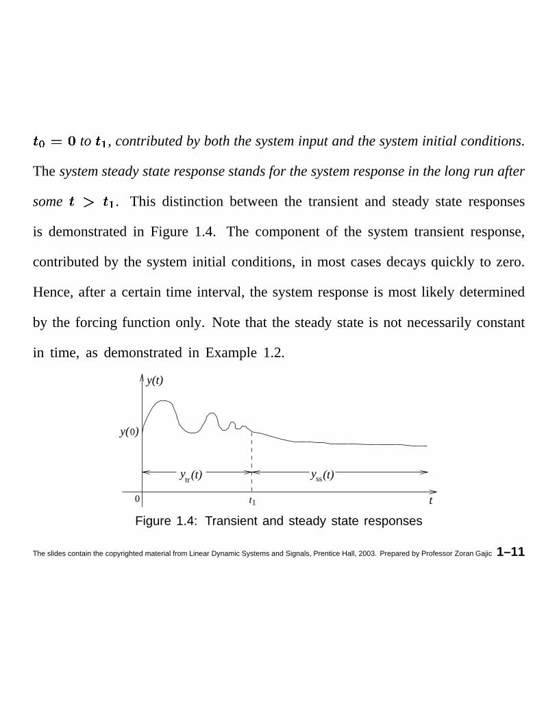
Example 1.2: Considerthesamesystemasin Example1.1 with thesameinitial

conditions,but take the forcing function as , that is

##

The solution is derived in the textbookas

$&% $(')%

It is easyto seethat thesystemresponseexponentialfunctionsdecayto zeropretty

rapidly so that the systemsteadystateresponseis determinedby

*+* ,


The plots of and -+- are given in Figure 1.5.

0 5 10 15−0.4

−0.2

0

0.2

0.4

0.6

0.8

1

1.2

time in seconds

syst

em r

espo

nse

y(t)

yss(t)

Figure 1.5: System complete response (solid line) and

its steady state response (dashed line) for Example 1.2

It can be seenfrom the abovefigure that the transientendsroughly at . ,

henceafter that time the systemis in its steadystate.


Linear dynamic systemsprocessinput signalsin order to produceoutput sig-

nals. The processingrule is given in the form of differential/differenceequations.

Sometimes,linear dynamic systemsare called linear signal processors.A block

diagramrepresentationof a linear system,processingoneinput andproducingone

output, is given in Figure 1.6.

y

Input OutputLinear System

f

Figure 1.6: Input–output block diagram of a system


In general,thesysteminput signalcanbedifferentiatedby thesystemso that the

moregeneraldescriptionof time invariant linear continuous-timesystemsis/

/ /�0�1/�0�1

/�0�1 1 2

33

3 340�1340�1

340�1 1 2

This systemdifferentiationof input signalsleadsto someinterestingsystemprop-

erties (to be discussedin Chapters3 and 4). The correspondinggeneralform of

time invariant linear discrete-timesystemsis

/�0�1 1 2

3 350�1 1 2

Thecoefficients 6 and 7 areconstants.

Note that for real physicalsystems .


Dueto thepresenceof thederivativesof theinputsignalon theright-handsideof

thegeneralsystemequation,impulsesthat instantlychangesysteminitial conditions

are generatedat the initial time. Theseimpulsesare called the impulse delta

functions(signals).The impulsedeltasignalandits role in thederivativeoperation

will be studiedin detail in Chapter2. We will learn in this textbook a method

for solving the considereddifferential equationsbasedon the Laplacetransform.

The Laplacetransformwill bepresentedin Chapter4. Anothermethodfor solving

the generalsystemdifferential equationrequiresusing 8 9with theparticular solutionbeingobtainedthroughtheconvolutionoperation. The

convolutionoperationwill be introducedin Chapter2 andusedin Chapters3 and

4 for analysisof linear time invariant systems. The convolution operationwill

be studiedin detail in Chapter6 and its usein linear systemtheory will be fully

demonstratedin Sections7.1 and 8.2.


The problemof finding the systemresponsefor the given input signal or

is the central problemin the analysisof linear systems. It is basically the

problemof solvingthecorrespondinglineardifferentialor differenceequation.This

problemcanbe solvedeitherby usingknowledgefrom the mathematicaltheoryof

linear differentialand/ordifferenceequationsor the engineeringfrequencydomain

approach—basedon the conceptof the systemtransfer function, which leadsto

the conclusionthat linear systemscanbe studiedeither in the time domain(to be

generalizedin Chapter8 to the statespaceapproach)or in the frequencydomain

(transferfunctionapproach).Chapters3–5of this textbookwill bededicatedto the

frequencydomaintechniquesandChapters6–8 will studytime domaintechniques

for the analysisof continuous-anddiscrete-timelinear time-invariantsystems.


The systemconsideredso far and symbolically representedin Figure 1.6, has

only oneinput andoneoutput . Suchsystemsareknownassingle-inputsingle-

outputsystems. In general,systemsmay haveseveralinputs and severaloutputs,

say inputs : ; < , and outputs, : ; = . Thesesystemsareknown

asmulti-input multi-outputsystems. They arealsocalledmultivariablesystems. A

block diagramfor a multi-input multi-outputsystemis representedin Figure1.7.

y1y2

f1f2 . . .

. . .

Linear System

f ypr

Figure 1.7: Block diagram of a multi-input multi-output system

The problem of obtaining differential (difference)equationsthat describedy-

namicsof realphysicalsystemsis knownasmathematicalmodeling. In Section1.3

mathematicalmodelsfor severalreal physicalsystemswill be derived.


1.2 System Linearity and Time Invariance

In Section1.1, the conceptof systemlinearity is tacitly introducedby statingthat

linear dynamic systemsare describedby linear differential/differenceequations.

We have also statedthat the conceptof time invarianceis related to differen-

tial/differenceequationswith constantcoefficients. In this sectionwe discussthe

conceptsof systemlinearity and time invariancein more details.

1.2.1 SystemLinearity

The conceptof systemlinearity is presentedfor continuous-timesystems.Similar

derivationsand explanationsare valid for presentationof the linearity conceptof

discrete-timelineardynamicsystems.Beforewe deriveandstatethelinearity prop-

erty of continuous-timelinear dynamicsystems,we needthe following definition.

Definition 1.3: Thesystemat restis thesystemthathasno initial internalenergy,

that is, all its initial conditionsare equal to zero.


It follows from Definition 1.3 that for a systemat rest,the initial conditionsare

set to zero, that is

> > ?�@�A >?�@�A

Systemsat rest arealsocalled systemswith zero initial conditions.

The linearity propertyof continuous-timelinear dynamicsystemsis the conse-

quenceof the linearity propertyof mathematicalderivatives,that isBB A

BB C

BB A C

Considerthe general th order continuous-timelinear differential equationthat

describesthe behaviorof an th order linear dynamic system. Assumethat the

systemis at rest, and that it is driven eitherby A or C , which respectively

producethe systemoutputs A and C , that is


D ED D�F E

D�F E ED�F E E E

G E

HH E

H H4F EH5F E E

H4F E E EG E

andD I

D D�F ED�F E I

D�F E E IG I

HH I

H H4F EH4F E I

H5F E E IG I

Assumenow that the samesystemat rest is driven by a linear combinationE I

where and are known constants. Multiplying the first

equationby and multiplying the secondequationby and adding the two

differential equations,we obtain the following differential equation


J K LJ JM K

J�M K K LJ�M K N K L

OO K L

O O4M KO4M K K L

O5M K

N K L

It is easyto concludethat the output of the systemat rest (the solution of the

correspondingdifferential equation)due to a linear combinationof systeminputsK L

is equalto thecorrespondinglinearcombinationof thesystemof

outputs,that isK L

. This is basicallythe linearity principle. Notethat

thelinearityprincipleis valid undertheassumptionthatthesysteminitial conditions

are zero (systemat rest). The linearity principle is, in fact, the superposition

principle, the well known principle of elementarycircuit theory.


Thelinearityprinciplecanbeput in a formalmathematicalframeworkasfollows.

If we introducethesymbolicnotation,thesolutionsof theconsideredequationscan

be recordedas

P P Q Q

where standsfor a linear integral type operator. In order to get a solution of

an th order differential equation,the correspondingdifferential equationhas to

be integrated -times. That is why, linear dynamicsystemscan be modelledas

integrators. Note that the considereddifferential equationscan be multiplied by

someconstants,say and producing

P P P

Q Q Q


Adding theseequationsleadsto the conclusionthat

R S R S

It follows that the linearity principle canbe mathematicallystatedasfollows

R S R S

Usingasimilar reasoning,wecanstatethelinearityprinciplefor anarbitrarynumber

of inputs, that is

R R S S T T

R R S S T T

where U are constants.


The linearity principle is demonstratedgraphicallyin Figure1.8.

yα 1(t)

The SameLinear System

The SameLinear System

++

(t) y (t)2

yα 1(t) y (t)

2(t)

Linear System

β2

2

β

β β

1(t)

1(t)

f

f

α

ffα

1.8: Graphical representation of the linearity principle for a system at rest

It is straightforwardto verify, by usingsimilar argumentsthat the linear difference

equationalso obeysto the linearity principle, that isV V W W X X

V V W W X X

where Y are constants.


1.2.2 Linear SystemTime Invariance

For a general th order linear dynamicsystem,representedby

ZZ Z�[]\

Z�[�\Z�[�\ Z�[(^

Z�[�^Z�[�^ \ _

``

` `5[�\`5[�\

`5[�\ \ _

thecoefficients a , and a , areassumed

to be constant,which indicatesthat the given systemis time invariant.

Here,we give anadditionalclarificationof thesystemtime invariance.Consider

a systemat rest. The systemtime invarianceis manifestedby theconstantshapein

time (waveform)of the systemoutput responsedueto the given input. The output

responseof a systemat restis invariantregardlessof the initial time of the input. If

thesysteminput is shiftedin time, thesystemoutputresponsedueto thesameinput

will be shifted in time by the sameamountand, in addition, it will preservethe


samewaveform. The correspondinggraphicalinterpretationof the time invariance

principle is shown in Figure 1.9.

b c

dfehg i

j klfmhnpoqnsr

t uv w

xzy|{ }

~ ��z�|��

� �

��

��

¢¡�£¥¤�¦�§£¨�©�ª�«�¬��®�¯�°�±�«�²

³z´qµ ¶

·z¸q¹�º�¹¼»

½¢¾�¿ À

Á¢Â�ÃÅÄÆÃÈÇÉ Ê

Figure 1.9: Graphical representation of system time invariance

The sameargumentspresentedfor the time invarianceof continuous-timelinear

dynamicsystems,describedby differential equations,hold for the time invariance

of discrete-timelinear dynamicsystemsdescribedby differenceequations.

The systemlinearity and time invarianceprincipleswill be usedin the follow

up chaptersto simplify the solution to the main linear systemtheoryproblem,the

problemof finding the systemresponsedueto arbitrary input signals.


1.3 Mathematical Modeling of Systems

An Electrical Cir cuit

Considera simpleRLC electricalcircuit presentedin Figure1.10.

ei

R1

i2

R2 eo

i1

i3

L

C

Figure 1.10: An RLC network

Applying the basiccircuit laws for voltagesandcurrents,we obtain

Ë Ì Ì Ì Í


and

Î Ï ÏÐ

ÎÑ Ò Ñ Î

Ó Ï Ñ

It follows from the aboveequationsthat

Ó Ï Î Î

Fromtheseequationsweobtainthedesiredsecond-orderdifferentialequation,which

relatesthe input andoutputof the system,andrepresentsa mathematicalmodelof

the circuit given in Figure 1.10


Ô ÕÔ

Ö ÔÔ

Õ Ö ÔÔ

Õ ×

In orderto beableto solvethis differentialequationforÕ

, the initial conditionsÕ

andÕ

must be known (determined). For electrical circuits, the

initial conditionsare usually specifiedin termsof capacitorvoltagesand inductor

currents. Hence,in this example,Õ

andÕ

shouldbe expressedin

termsof Ø and Ö . Note that in this mathematicalmodel×

represents

the systeminput andÕ

is the systemoutput. However,anyof the currentsand

any of the voltagescanplay the rolesof either input or outputvariables.


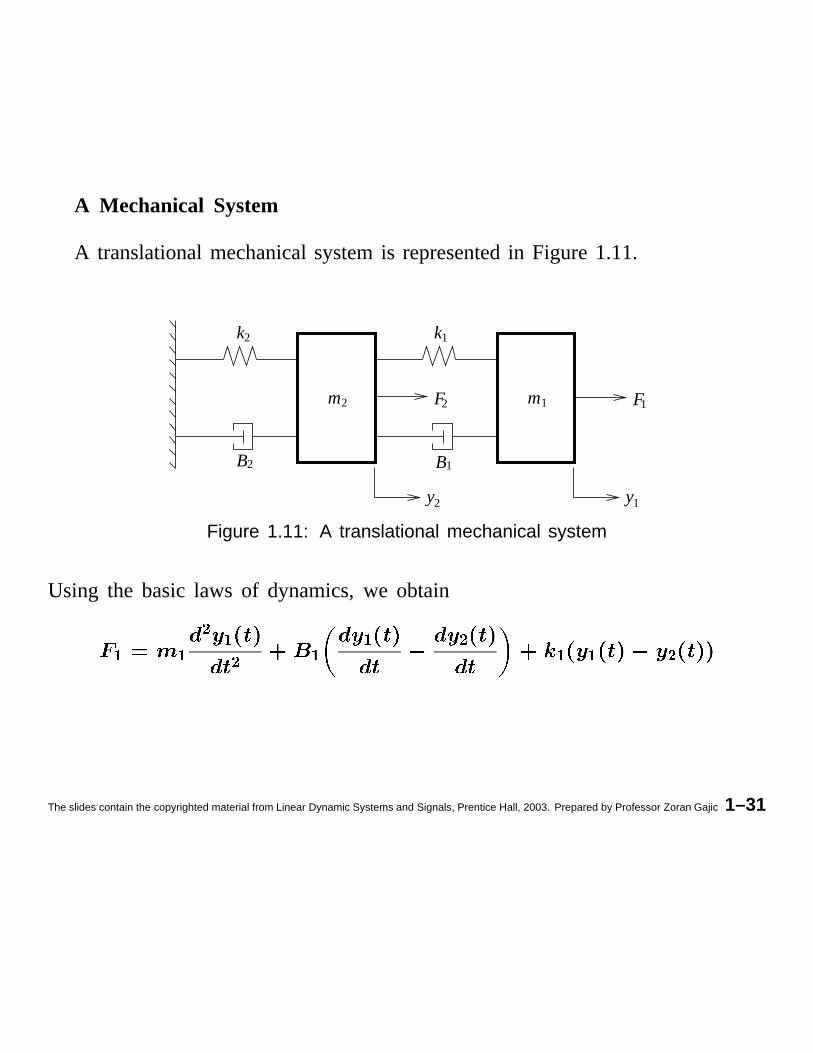
A Mechanical System

A translationalmechanicalsystemis representedin Figure 1.11.

B2

y1

m2

k1k2

F1

y2

1B

m1F2

Figure 1.11: A translational mechanical system

Using the basic laws of dynamics,we obtain

Ù ÙÚ Ù

Ú Ù Ù Ú Ù Ù Ú


and

Û ÛÛ Û

Û Û Û Û Û Ü Ü Û

Ü Ü Û

This systemhastwo inputs, Ü and Û , and two outputs, Ü and Û . These

equationscan be rewritten as

ÜÛ Ü

Û Ü Ü Ü Ü Ü Û Ü Û Ü

andÜ Ü Ü Ü Û

Û ÛÛ Ü Û Û

Ü Û Û Û

Techniquesfor obtainingexperimentallymathematicalmodelsof dynamicsys-

temsarestudiedwithin the scientific areacalled systemidentification.


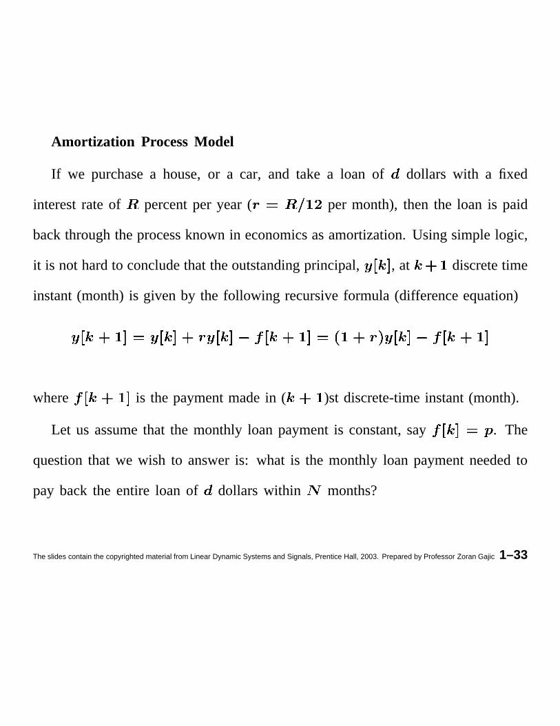
Amortization ProcessModel

If we purchasea house,or a car, and take a loan of dollars with a fixed

interestrate of percentper year ( per month), then the loan is paid

backthroughtheprocessknown in economicsasamortization.Usingsimplelogic,

it is not hardto concludethat theoutstandingprincipal, , at discretetime

instant(month) is given by the following recursiveformula (differenceequation)

where is the paymentmadein ( )st discrete-timeinstant(month).

Let us assumethat the monthly loan paymentis constant,say . The

questionthat we wish to answeris: what is the monthly loan paymentneededto

pay back the entire loan of dollars within months?


The answerto this questioncan be easily obtain by iterating this difference

equationand finding the correspondingsolution formula. Since and

areknown, we havefor and

Ý

Continuingthis procedurefor we canrecognizethe patternandget

Þ Ý

ß ßáà�â Ý

ß ßãà�â

äæåèçä


The formula obtainedrepresentsthe solution of the differenceequation. The

formula canbe evenfurther simplified using the known summationformulaé

êæëèìê éîí�ï

Applying this formula, we obtain

ð ð ð ð

We concludethat the loanis paidbackwhen , which impliestheformula

for the requiredmonthly paymentas

ð ð ðð


Heart Beat Dynamics

Dynamicsof a heartbeat(diastoleis a relaxedstateandsystoleis a contracted

stateof a heart) can be approximatelydescribedby the following set of linear

differential equations

ñ ñ ò ó

ò ñ ò

ó ò

where ñ is the lengthof musclefibre, ò representsthe tensionin the fiber

causedby blood pressure,and ó representsdynamicsof an electrochemical

processthatgovernstheheartbeat,and is a smallpositiveparameter.Thesystem

is drivenby the initial conditionthat characterizesthe heart’sdiastolicstate,whose

normalizedvalue,in this model,is equalto ñ ò ó .


Eye Movement (Oculomotor Dynamics)

Dynamicsof eye movement(muscles,eye, and orbit) can be modeledby the

second-ordersystemrepresentedbyô

ô õ ô õ ô õ ô

whereõ

and ô are respectivelythe minor and major eye

time constants. is the eye position in degreesand is the eye stimulus

forcein degrees(referenceeyeposition,targetposition). Severalothermathematical

modelsfor eyemovementexist in the biomedicalengineeringliterature,including

a morecomplexmodelof ordersix to be presentedin Chapter8, Problem8.46.


BOEING Air craft

The linearizedequationsgoverningthe motion of a BOEING’s aircraft are

ö

ö

where in theaircraftangleof attack, is thepitch rate,and represents

the aircraft pitch angle. The driving force ö standsfor the elevatordeflection

angle. Dif ferentiating the above system of three first-order linear differential

equations,it can be replacedby one third-order linear differential equationthat

gives direct dependenceof on ö , that is÷

÷ø

øö ö


1.4 SystemClassification

Real-world systemsare either static or dynamic. Static systemsare represented

by algebraicequations,for examplealgebraicequationsdescribingelectrical cir-

cuits with resistorsand constantvoltagesources,or algebraicequationsin statics

indicating that at the equilibrium the sumsof all forcesareequalto zero.

Dynamic systemsare, in general, describedeither by differential/difference

equations(alsoknown assystems with concentrated or lumped parameters) or by

partial differential equations(known as systems with distributed parameters). For

example,electricpowertransmissionlines,wavepropagation,behaviorof antennas,

propagationof light throughoptical fiber, and heatconductionrepresentdynamic

systemsdescribedby partial differential equations.For example,onedimensional

electromagneticwavepropagationis describedby the partial differentialequation


ùù

ù ùù

is electricfiled, representstime, is the spacialcoordinateand is the

constantthat characterizesthe medium. Systemswith distributedparametersare

alsoknownasinfinitedimensionalsystems, in contrastto systemswith concentrated

parametersthat are known as finite dimensionalsystems(they are representedby

differential/differenceequationsof finite orders, ).

Dynamic systemswith lumped parameterscan be either linear or nonlinear.

Linear dynamic systems are describedby linear differential/differenceequations

andthey obeyto the linearity principle. Nonlinear dynamic systems aredescribed

by nonlineardifferential/differenceequations.For example,a simple pendulumis

describedby the nonlineardifferential equation


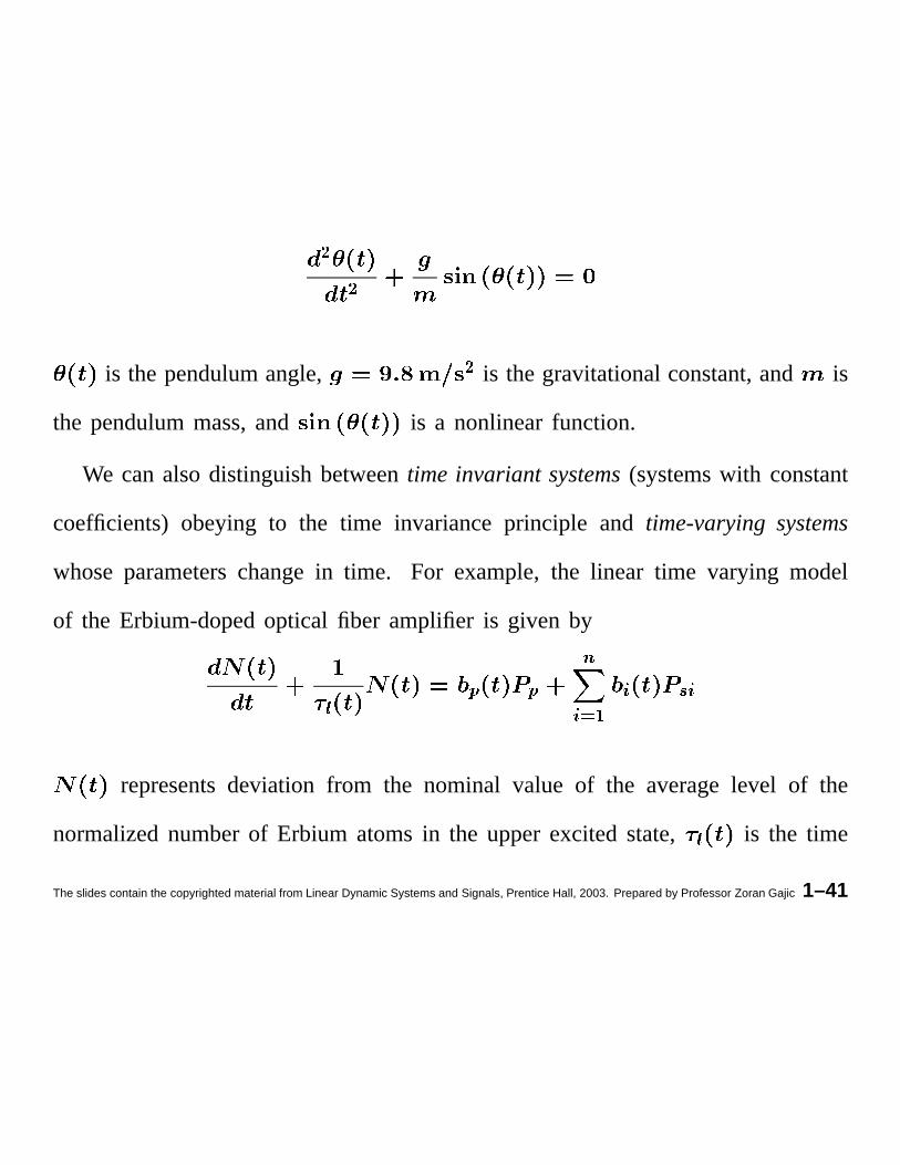
úú

is the pendulumangle,ú

is the gravitationalconstant,and is

the pendulummass,and is a nonlinearfunction.

We canalsodistinguishbetweentime invariant systems(systemswith constant

coefficients) obeying to the time invarianceprinciple and time-varyingsystems

whoseparameterschangein time. For example,the linear time varying model

of the Erbium-dopedoptical fiber amplifier is given by

û ü üý

þæÿ��þ ��þ

representsdeviation from the nominal value of the averagelevel of the

normalizednumberof Erbium atomsin the upperexcitedstate, û is the time


varying time constant, � and �� are respectivelylaserpump and optical signal

powerdeviationsfrom their nominalvalues,and � and � arecoefficients.

Somesystemparametersand variablescan changeaccordingto randomlaws.

For example,the generatedpowerof a solarcell, househumidity andtemperature.

Sometimessysteminputs are randomsignals. For example,aircraft under wind

disturbances,electric current under electron thermal noise. Systemsthat have

randomparametersand/or processrandomsignalsare called stochastic systems.

Stochasticsystemscanbeeitherlinearor nonlinear,time invariantor time-varying,

continuousor discrete. In contrastto stochasticsystems,we have deterministic

systems whoseparametersand input signalsaredeterministicquantities.

Real world physicalsystemsare known as nonanticipatory systems or causal

systems. Let the input � be appliedto a systemat time � . The real physical

systemcan only to producethe systemoutput at time equal to � , that is � .


The real physicalsystemcannot,at time � , produceinformation about for

� . That is, thesystemis unableto predictthe future input valuesandproduce

the future systemresponse , basedon the information that the systemhas

at time � . The systemcausalitycan also be defined with the statementthat the

systeminput hasno impact on the systemoutput � for � . In

contrastto nonanticipatory(causal)systems,we have anticipatory or noncausal

systems. Anticipatory systemsare encounteredin digital signal processing—they

are artificial systems.

Dynamic systemsare also systems with memory. Namely, the systemoutput

at time � dependsnot only on the system input at time � , but also on all

previousvaluesof the systeminput. Let be the solution of

the correspondingdifferential equationrepresentinga dynamicsystem.


The fact that the dynamicsystempossessesmemorycan be formally recordedas

� . In contrast,static systemshaveno memory. If

the relationship camefrom a static system,thenwe would have

. That is, for staticsystemsthe outputat time dependsonly

on the input at the given time instant . Staticsystemsareknown asmemoryless

systems or instantaneous systems. For example,an electric resistor is a static

systemsinceits voltage(systemoutput) is an instantaneousfunction of its current

(systeminput) so that for any .

Analog systems dealwith continuous-timesignalsthat cantakea continuumof

valueswith respectto the signalmagnitude.Digital systems processdigital signals

whosemagnitudescan take only a finite numberof values. In digital systems,

signalsare discretizedwith respectto both time and magnitude(signal sampling

and quantization).


Documents

1.1 Continuous and Discrete Signals and Systems A continuous signal