Embed Size (px)
Citation preview
10.6 Other Heat Conduction Problems 581
(a) Let u(x, t) = eδtw(x, t), where δ is constant, and find the corresponding partial dif-ferential equation for w.(b) If b �= 0, show that δ can be chosen so that the partial differential equation found inpart (a) has no term in w. Thus, by a change of dependent variable, it is possible to reduceEq. (i) to the heat conduction equation.
22. The heat conduction equation in two space dimensions is
α2(uxx + uyy) = ut .
Assuming that u(x, y, t) = X (x)Y (y)T (t), find ordinary differential equations satisfiedby X (x), Y (y), and T (t).
23. The heat conduction equation in two space dimensions may be expressed in terms of polarcoordinates as
α2[urr + (1/r)ur + (1/r2)uθθ
] = ut .
Assuming that u(r, θ, t) = R(r)�(θ)T (t), find ordinary differential equations satisfied byR(r), �(θ), and T (t).
10.6 Other Heat Conduction Problems
In Section 10.5 we considered the problem consisting of the heat conduction equation
α2uxx = ut , 0 < x < L , t > 0, (1)
the boundary conditions
u(0, t) = 0, u(L , t) = 0, t > 0, (2)
and the initial condition
u(x, 0) = f (x), 0 ≤ x ≤ L . (3)
We found the solution to be
u(x, t) =∞∑
n=1
cne−n2π2α2t/L2sin
nπx
L, (4)
where the coefficients cn are the same as in the series
f (x) =∞∑
n=1
cn sinnπx
L. (5)
The series in Eq. (5) is just the Fourier sine series for f ; according to Section 10.4 itscoefficients are given by
cn = 2
L
∫ L
0f (x) sin
nπx
Ldx . (6)
Hence the solution of the heat conduction problem, Eqs. (1) to (3), is given by theseries in Eq. (4) with the coefficients computed from Eq. (6).
We emphasize that at this stage the solution (4) must be regarded as a formal solution;that is, we obtained it without rigorous justification of the limiting processes involved.

582 Chapter 10. Partial Differential Equations and Fourier Series
Such a justification is beyond the scope of this book. However, once the series (4)has been obtained, it is possible to show that in 0 < x < L , t > 0 it converges to acontinuous function, that the derivatives uxx and ut can be computed by differentiatingthe series (4) term by term, and that the heat conduction equation (1) is indeed satisfied.The argument rests heavily on the fact that each term of the series (4) contains a negativeexponential factor, and this results in relatively rapid convergence of the series. A furtherargument establishes that the function u given by Eq. (4) also satisfies the boundaryand initial conditions; this completes the justification of the formal solution.
It is interesting to note that although f satisfies the conditions of the Fourier con-vergence theorem (Theorem 10.3.1), it may have points of discontinuity. In this casethe initial temperature distribution u(x, 0) = f (x) is discontinuous at one or morepoints. Nevertheless, the solution u(x, t) is continuous for arbitrarily small values oft > 0. This illustrates the fact that heat conduction is a diffusive process that instantlysmooths out any discontinuities that may be present in the initial temperature distribu-tion. Finally, since f is bounded, it follows from Eq. (6) that the coefficients cn are alsobounded. Consequently, the presence of the negative exponential factor in each termof the series (4) guarantees that
limt→∞ u(x, t) = 0 (7)
for all x regardless of the initial condition. This is in accord with the result expectedfrom physical intuition.
We now consider two other problems of one-dimensional heat conduction that canbe handled by the method developed in Section 10.5.
Nonhomogeneous Boundary Conditions. Suppose now that one end of the bar is heldat a constant temperature T1 and the other is maintained at a constant temperature T2.Then the boundary conditions are
u(0, t) = T1, u(L , t) = T2, t > 0. (8)
The differential equation (1) and the initial condition (3) remain unchanged.This problem is only slightly more difficult, because of the nonhomogeneous bound-
ary conditions, than the one in Section 10.5. We can solve it by reducing it to a problemhaving homogeneous boundary conditions, which can then be solved as in Section10.5. The technique for doing this is suggested by the following physical argument.
After a long time, that is, as t → ∞, we anticipate that a steady temperature distribu-tion v(x) will be reached, which is independent of the time t and the initial conditions.Since v(x) must satisfy the equation of heat conduction (1), we have
v′′(x) = 0, 0 < x < L . (9)
Hence the steady-state temperature distribution is a linear function of x . Further, v(x)must satisfy the boundary conditions
v(0) = T1, v(L) = T2, (10)
which are valid even as t → ∞. The solution of Eq. (9) satisfying Eqs. (10) is
v(x) = (T2 − T1)x
L+ T1. (11)
10.6 Other Heat Conduction Problems 583
Returning to the original problem, Eqs. (1), (3), and (8), we will try to express u(x, t)as the sum of the steady-state temperature distribution v(x) and another (transient)temperature distribution w(x, t); thus we write
u(x, t) = v(x)+ w(x, t). (12)
Since v(x) is given by Eq. (11), the problem will be solved provided we can determinew(x, t). The boundary value problem forw(x, t) is found by substituting the expressionin Eq. (12) for u(x, t) in Eqs. (1), (3), and (8).
From Eq. (1) we have
α2(v + w)xx = (v + w)t ;it follows that
α2wxx = wt , (13)
since vxx = 0 and vt = 0. Similarly, from Eqs. (12), (8), and (10),
w(0, t) = u(0, t)− v(0) = T1 − T1 = 0,(14)
w(L , t) = u(L , t)− v(L) = T2 − T2 = 0.
Finally, from Eqs. (12) and (3),
w(x, 0) = u(x, 0)− v(x) = f (x)− v(x), (15)
where v(x) is given by Eq. (11). Thus the transient part of the solution to the originalproblem is found by solving the problem consisting of Eqs. (13), (14), and (15). Thislatter problem is precisely the one solved in Section 10.5 provided that f (x)− v(x) isnow regarded as the initial temperature distribution. Hence
u(x, t) = (T2 − T1)x
L+ T1 +
∞∑n=1
cne−n2π2α2t/L2sin
nπx
L, (16)
where
cn = 2
L
∫ L
0
[f (x)− (T2 − T1)
x
L− T1
]sin
nπx
Ldx . (17)
This is another case in which a more difficult problem is solved by reducing it to asimpler problem that has already been solved. The technique of reducing a problem withnonhomogeneous boundary conditions to one with homogeneous boundary conditionsby subtracting the steady-state solution is capable of wide application.
E X A M P L E
1
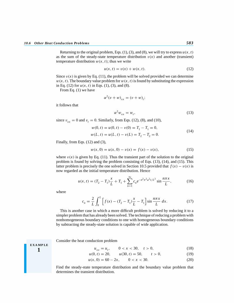
Consider the heat conduction problem
uxx = ut , 0 < x < 30, t > 0, (18)
u(0, t) = 20, u(30, t) = 50, t > 0, (19)
u(x, 0) = 60 − 2x, 0 < x < 30. (20)
Find the steady-state temperature distribution and the boundary value problem thatdetermines the transient distribution.
584 Chapter 10. Partial Differential Equations and Fourier Series
The steady-state temperature satisfies v′′(x) = 0 and the boundary conditions v(0) =20 and v(30) = 50. Thus v(x) = 20 + x . The transient distribution w(x, t) satisfiesthe heat conduction equation
wxx = wt , (21)
the homogeneous boundary conditions
w(0, t) = 0, w(30, t) = 0, (22)
and the modified initial condition
w(x, 0) = 60 − 2x − (20 + x) = 40 − 3x . (23)
Note that this problem is of the form (1), (2), (3) with f (x) = 40 − 3x , α2 = 1, andL = 30. Thus the solution is given by Eqs. (4) and (6).
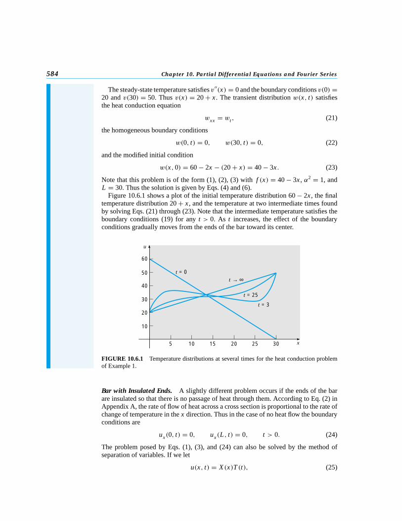
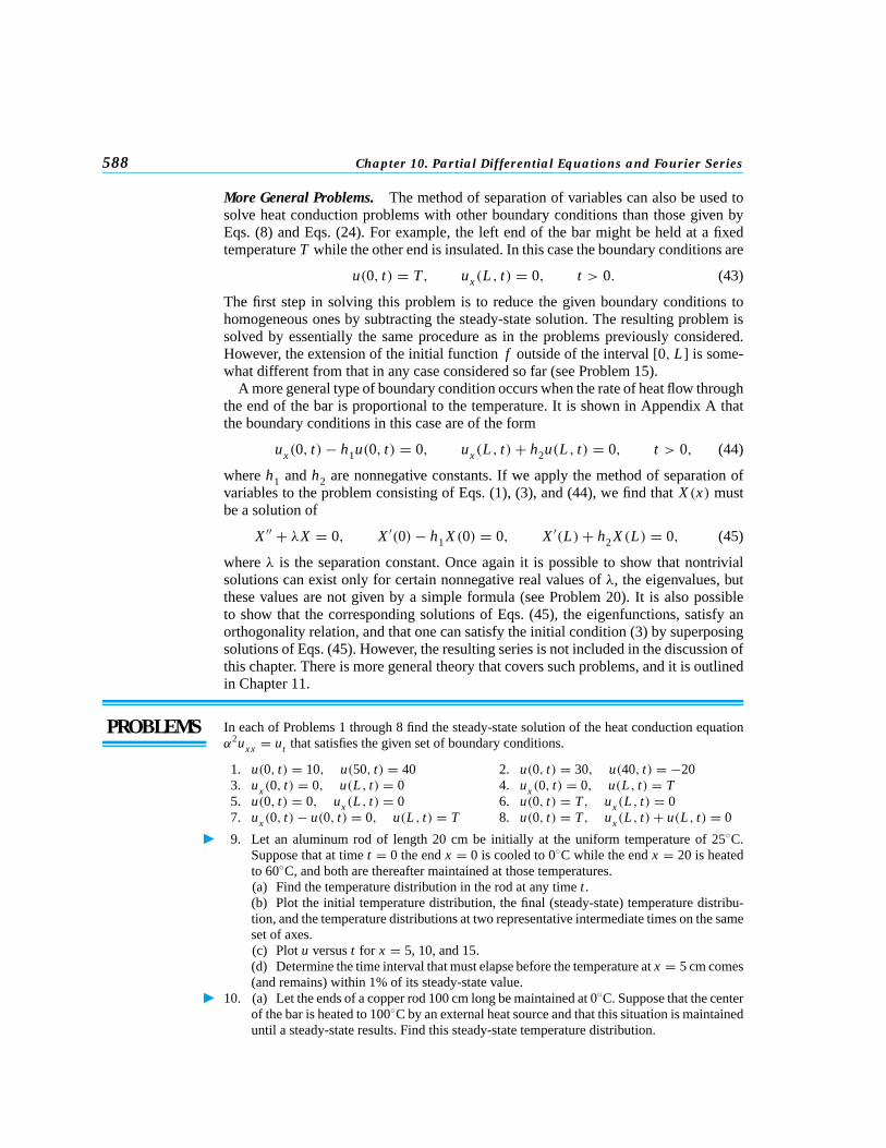
Figure 10.6.1 shows a plot of the initial temperature distribution 60 − 2x , the finaltemperature distribution 20 + x , and the temperature at two intermediate times foundby solving Eqs. (21) through (23). Note that the intermediate temperature satisfies theboundary conditions (19) for any t > 0. As t increases, the effect of the boundaryconditions gradually moves from the ends of the bar toward its center.
302510 155 20
60
50
40
30
20
10
u
x
t = 0
t = 25
t = 3
t → ∞
FIGURE 10.6.1 Temperature distributions at several times for the heat conduction problemof Example 1.
Bar with Insulated Ends. A slightly different problem occurs if the ends of the barare insulated so that there is no passage of heat through them. According to Eq. (2) inAppendix A, the rate of flow of heat across a cross section is proportional to the rate ofchange of temperature in the x direction. Thus in the case of no heat flow the boundaryconditions are
ux(0, t) = 0, ux(L , t) = 0, t > 0. (24)
The problem posed by Eqs. (1), (3), and (24) can also be solved by the method ofseparation of variables. If we let
u(x, t) = X (x)T (t), (25)
10.6 Other Heat Conduction Problems 585
and substitute for u in Eq. (1), then it follows as in Section 10.5 that
X ′′
X= 1
α2
T ′
T= −λ, (26)
where λ is a constant. Thus we obtain again the two ordinary differential equations
X ′′ + λX = 0, (27)
T ′ + α2λT = 0. (28)
For any value of λ a product of solutions of Eqs. (27) and (28) is a solution of thepartial differential equation (1). However, we are interested only in those solutions thatalso satisfy the boundary conditions (24).
If we substitute for u(x, t) from Eq. (25) in the boundary condition at x = 0, weobtain X ′(0)T (t) = 0. We cannot permit T (t) to be zero for all t , since then u(x, t)would also be zero for all t . Hence we must have
X ′(0) = 0. (29)
Proceeding in the same way with the boundary condition at x = L , we find that
X ′(L) = 0. (30)
Thus we wish to solve Eq. (27) subject to the boundary conditions (29) and (30). It ispossible to show that nontrivial solutions of this problem can exist only if λ is real. Oneway to show this is indicated in Problem 18; alternatively, one can appeal to a moregeneral theory to be discussed later in Section 11.2. We will assume that λ is real andconsider in turn the three cases λ < 0, λ = 0, and λ > 0.
If λ < 0, it is convenient to let λ = −µ2, where µ is real and positive. Then Eq. (27)becomes X ′′ − µ2 X = 0 and its general solution is
X (x) = k1 sinhµx + k2 coshµx . (31)
In this case the boundary conditions can be satisfied only by choosing k1 = k2 = 0.Since this is unacceptable, it follows that λ cannot be negative; in other words, theproblem (27), (29), (30) has no negative eigenvalues.
If λ = 0, then Eq. (27) is X ′′ = 0, and therefore
X (x) = k1x + k2. (32)
The boundary conditions (29) and (30) require that k1 = 0 but do not determine k2.Thus λ = 0 is an eigenvalue, corresponding to the eigenfunction X (x) = 1. For λ = 0it follows from Eq. (28) that T (t) is also a constant, which can be combined with k2.Hence, for λ = 0, we obtain the constant solution u(x, t) = k2.
Finally, if λ > 0, let λ = µ2, where µ is real and positive. Then Eq. (27) becomesX ′′ + µ2 X = 0, and consequently
X (x) = k1 sinµx + k2 cosµx . (33)
The boundary condition (29) requires that k1 = 0, and the boundary condition (30)requires that µ = nπ/L for n = 1, 2, 3, . . . , but leaves k2 arbitrary. Thus the problem(27), (29), (30) has an infinite sequence of positive eigenvalues λ = n2π2/L2 with thecorresponding eigenfunctions X (x) = cos(nπx/L). For these values of λ the solutionsT (t) of Eq. (28) are proportional to exp(−n2π2α2t/L2).
586 Chapter 10. Partial Differential Equations and Fourier Series
Combining all these results, we have the following fundamental solutions for theproblem (1), (3), and (24):
u0(x, t) = 1,(34)
un(x, t) = e−n2π2α2t/L2cos
nπx
L, n = 1, 2, . . . ,
where arbitrary constants of proportionality have been dropped. Each of these functionssatisfies the differential equation (1) and the boundary conditions (24). Because boththe differential equation and boundary conditions are linear and homogeneous, anyfinite linear combination of the fundamental solutions satisfies them. We will assumethat this is true for convergent infinite linear combinations of fundamental solutions aswell. Thus, to satisfy the initial condition (3), we assume that u(x, t) has the form
u(x, t) = c0
2u0(x, t)+
∞∑n=1
cnun(x, t)
= c0
2+
∞∑n=1
cne−n2π2α2t/L2cos
nπx
L. (35)
The coefficients cn are determined by the requirement that
u(x, 0) = c0
2+
∞∑n=1
cn cosnπx
L= f (x). (36)
Thus the unknown coefficients in Eq. (35) must be the coefficients in the Fourier cosineseries of period 2L for f . Hence
cn = 2
L
∫ L
0f (x) cos
nπx
Ldx, n = 0, 1, 2, . . . . (37)
With this choice of the coefficients c0, c1, c2, . . . , the series (35) provides the so-lution to the heat conduction problem for a rod with insulated ends, Eqs. (1), (3),and (24).
It is worth observing that the solution (35) can also be thought of as the sum of asteady-state temperature distribution (given by the constant c0/2), which is independentof time t , and a transient distribution (given by the rest of the infinite series) that vanishesin the limit as t approaches infinity. That the steady-state is a constant is consistentwith the expectation that the process of heat conduction will gradually smooth out thetemperature distribution in the bar as long as no heat is allowed to escape to the outside.The physical interpretation of the term
c0
2= 1
L
∫ L
0f (x) dx (38)
is that it is the mean value of the original temperature distribution.
10.6 Other Heat Conduction Problems 587
E X A M P L E
2
Find the temperature u(x, t) in a metal rod of length 25 cm that is insulated on theends as well as on the sides and whose initial temperature distribution is u(x, 0) = xfor 0 < x < 25.
The temperature in the rod satisfies the heat conduction problem (1), (3), (24) withL = 25. Thus, from Eq. (35), the solution is
u(x, t) = c0
2+
∞∑n=1
cne−n2π2α2t/625 cosnπx
25, (39)
where the coefficients are determined from Eq. (37). We have
c0 = 2
25
∫ 25
0x dx = 25 (40)
and, for n ≥ 1,
cn = 2
25
∫ 25
0x cos
nπx
25dx
= 50(cos nπ − 1)/(nπ)2 ={−100/(nπ)2, n odd;
0, n even.(41)
Thus
u(x, t) = 25
2− 100
π2
∞∑n=1,3,5,...
1
n2 e−n2π2α2t/625 cos(nπx/25) (42)
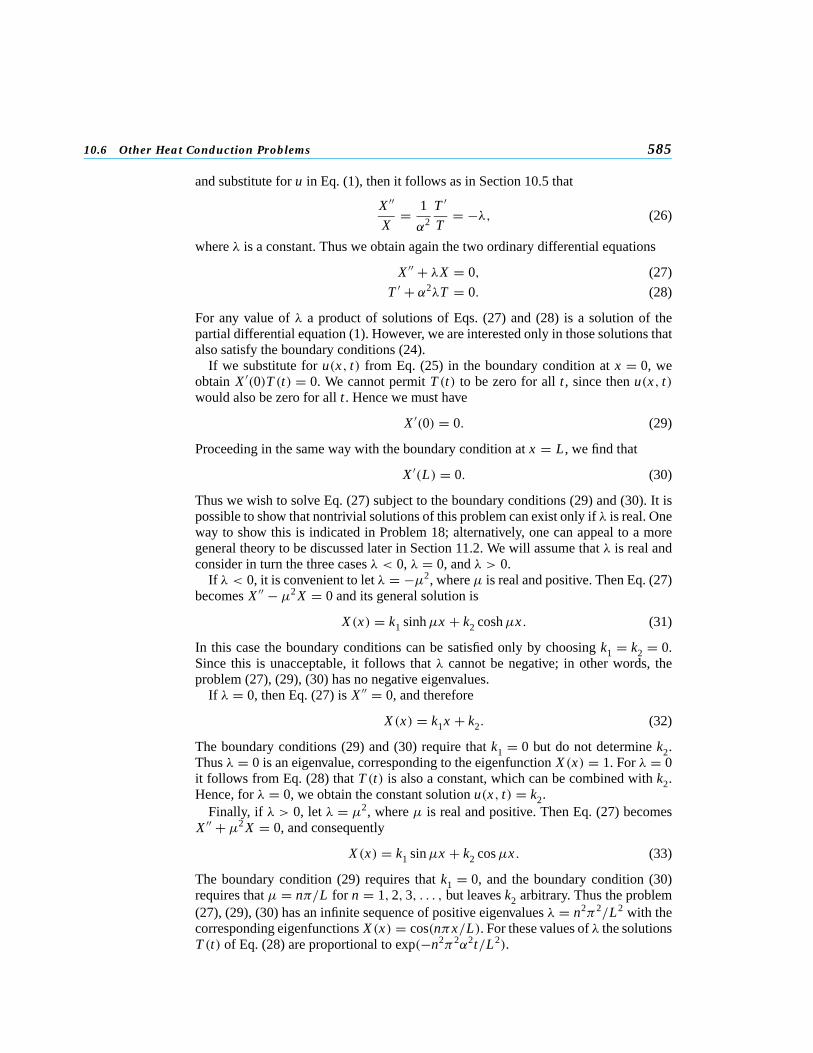
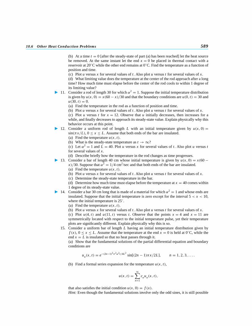
is the solution of the given problem.For α2 = 1 Figure 10.6.2 shows plots of the temperature distribution in the bar at
several times. Again the convergence of the series is rapid so that only a relatively fewterms are needed to generate the graphs.
2510 155 20
25
20
15
10
5
u
x
t = 0
t = 10
t = 40
t = 100t → ∞
FIGURE 10.6.2 Temperature distributions at several times for the heat conduction problemof Example 2.
588 Chapter 10. Partial Differential Equations and Fourier Series
More General Problems. The method of separation of variables can also be used tosolve heat conduction problems with other boundary conditions than those given byEqs. (8) and Eqs. (24). For example, the left end of the bar might be held at a fixedtemperature T while the other end is insulated. In this case the boundary conditions are
u(0, t) = T, ux(L , t) = 0, t > 0. (43)
The first step in solving this problem is to reduce the given boundary conditions tohomogeneous ones by subtracting the steady-state solution. The resulting problem issolved by essentially the same procedure as in the problems previously considered.However, the extension of the initial function f outside of the interval [0, L] is some-what different from that in any case considered so far (see Problem 15).
A more general type of boundary condition occurs when the rate of heat flow throughthe end of the bar is proportional to the temperature. It is shown in Appendix A thatthe boundary conditions in this case are of the form
ux(0, t)− h1u(0, t) = 0, ux(L , t)+ h2u(L , t) = 0, t > 0, (44)
where h1 and h2 are nonnegative constants. If we apply the method of separation ofvariables to the problem consisting of Eqs. (1), (3), and (44), we find that X (x) mustbe a solution of
X ′′ + λX = 0, X ′(0)− h1 X (0) = 0, X ′(L)+ h2 X (L) = 0, (45)
where λ is the separation constant. Once again it is possible to show that nontrivialsolutions can exist only for certain nonnegative real values of λ, the eigenvalues, butthese values are not given by a simple formula (see Problem 20). It is also possibleto show that the corresponding solutions of Eqs. (45), the eigenfunctions, satisfy anorthogonality relation, and that one can satisfy the initial condition (3) by superposingsolutions of Eqs. (45). However, the resulting series is not included in the discussion ofthis chapter. There is more general theory that covers such problems, and it is outlinedin Chapter 11.
PROBLEMS In each of Problems 1 through 8 find the steady-state solution of the heat conduction equationα2uxx = ut that satisfies the given set of boundary conditions.
1. u(0, t) = 10, u(50, t) = 40 2. u(0, t) = 30, u(40, t) = −203. ux (0, t) = 0, u(L , t) = 0 4. ux (0, t) = 0, u(L , t) = T5. u(0, t) = 0, ux (L , t) = 0 6. u(0, t) = T, ux (L , t) = 07. ux (0, t)− u(0, t) = 0, u(L , t) = T 8. u(0, t) = T, ux (L , t)+ u(L , t) = 0
� 9. Let an aluminum rod of length 20 cm be initially at the uniform temperature of 25◦C.Suppose that at time t = 0 the end x = 0 is cooled to 0◦C while the end x = 20 is heatedto 60◦C, and both are thereafter maintained at those temperatures.(a) Find the temperature distribution in the rod at any time t .(b) Plot the initial temperature distribution, the final (steady-state) temperature distribu-tion, and the temperature distributions at two representative intermediate times on the sameset of axes.(c) Plot u versus t for x = 5, 10, and 15.(d) Determine the time interval that must elapse before the temperature at x = 5 cm comes(and remains) within 1% of its steady-state value.
� 10. (a) Let the ends of a copper rod 100 cm long be maintained at 0◦C. Suppose that the centerof the bar is heated to 100◦C by an external heat source and that this situation is maintaineduntil a steady-state results. Find this steady-state temperature distribution.
10.6 Other Heat Conduction Problems 589
(b) At a time t = 0 [after the steady-state of part (a) has been reached] let the heat sourcebe removed. At the same instant let the end x = 0 be placed in thermal contact with areservoir at 20◦C while the other end remains at 0◦C. Find the temperature as a function ofposition and time.(c) Plot u versus x for several values of t . Also plot u versus t for several values of x .(d) What limiting value does the temperature at the center of the rod approach after a longtime? How much time must elapse before the center of the rod cools to within 1 degree ofits limiting value?
� 11. Consider a rod of length 30 for which α2 = 1. Suppose the initial temperature distributionis given by u(x, 0) = x(60 − x)/30 and that the boundary conditions are u(0, t) = 30 andu(30, t) = 0.(a) Find the temperature in the rod as a function of position and time.(b) Plot u versus x for several values of t . Also plot u versus t for several values of x .(c) Plot u versus t for x = 12. Observe that u initially decreases, then increases for awhile, and finally decreases to approach its steady-state value. Explain physically why thisbehavior occurs at this point.
� 12. Consider a uniform rod of length L with an initial temperature given by u(x, 0) =sin(πx/L), 0 ≤ x ≤ L . Assume that both ends of the bar are insulated.(a) Find the temperature u(x, t).(b) What is the steady-state temperature as t → ∞?(c) Let α2 = 1 and L = 40. Plot u versus x for several values of t . Also plot u versus tfor several values of x .(d) Describe briefly how the temperature in the rod changes as time progresses.
� 13. Consider a bar of length 40 cm whose initial temperature is given by u(x, 0) = x(60 −x)/30. Suppose that α2 = 1/4 cm2/sec and that both ends of the bar are insulated.(a) Find the temperature u(x, t).(b) Plot u versus x for several values of t . Also plot u versus t for several values of x .(c) Determine the steady-state temperature in the bar.(d) Determine how much time must elapse before the temperature at x = 40 comes within1 degree of its steady-state value.
� 14. Consider a bar 30 cm long that is made of a material for which α2 = 1 and whose ends areinsulated. Suppose that the initial temperature is zero except for the interval 5 < x < 10,where the initial temperature is 25◦.(a) Find the temperature u(x, t).(b) Plot u versus x for several values of t . Also plot u versus t for several values of x .(c) Plot u(4, t) and u(11, t) versus t . Observe that the points x = 4 and x = 11 aresymmetrically located with respect to the initial temperature pulse, yet their temperatureplots are significantly different. Explain physically why this is so.
15. Consider a uniform bar of length L having an initial temperature distribution given byf (x), 0 ≤ x ≤ L . Assume that the temperature at the end x = 0 is held at 0◦C, while theend x = L is insulated so that no heat passes through it.(a) Show that the fundamental solutions of the partial differential equation and boundaryconditions are
un(x, t) = e−(2n−1)2π2α2t/4L2sin[(2n − 1)πx/2L], n = 1, 2, 3, . . . .
(b) Find a formal series expansion for the temperature u(x, t),
u(x, t) =∞∑
n=1
cnun(x, t),
that also satisfies the initial condition u(x, 0) = f (x).Hint: Even though the fundamental solutions involve only the odd sines, it is still possible

590 Chapter 10. Partial Differential Equations and Fourier Series
to represent f by a Fourier series involving only these functions. See Problem 39 ofSection 10.4.
� 16. In the bar of Problem 15 suppose that L = 30, α2 = 1, and the initial temperature distri-bution is f (x) = 30 − x for 0 < x < 30.(a) Find the temperature u(x, t).(b) Plot u versus x for several values of t . Also plot u versus t for several values of x .(c) How does the location xm of the warmest point in the bar change as t increases? Drawa graph of xm versus t .(d) Plot the maximum temperature in the bar versus t .
� 17. Suppose that the conditions are as in Problems 15 and 16 except that the boundary conditionat x = 0 is u(0, t) = 40.(a) Find the temperature u(x, t).(b) Plot u versus x for several values of t . Also plot u versus t for several values of x .(c) Compare the plots you obtained in this problem with those from Problem 16. Explainhow the change in the boundary condition at x = 0 causes the observed differences in thebehavior of the temperature in the bar.
18. Consider the problem
X ′′ + λX = 0, X ′(0) = 0, X ′(L) = 0. (i)
Let λ = µ2, whereµ = ν + iσ with ν and σ real. Show that if σ �= 0, then the only solutionof Eqs. (i) is the trivial solution X (x) = 0.Hint: Use an argument similar to that in Problem 17 of Section 10.1.
19. The right end of a bar of length a with thermal conductivity κ1 and cross-sectional areaA1 is joined to the left end of a bar of thermal conductivity κ2 and cross-sectional area A2.The composite bar has a total length L . Suppose that the end x = 0 is held at temperaturezero, while the end x = L is held at temperature T . Find the steady-state temperature inthe composite bar, assuming that the temperature and rate of heat flow are continuous atx = a.Hint: See Eq. (2) of Appendix A.
20. Consider the problem
α2uxx = ut , 0 < x < L , t > 0;u(0, t) = 0, ux (L , t)+ γ u(L , t) = 0, t > 0; (i)
u(x, 0) = f (x), 0 ≤ x ≤ L .
(a) Let u(x, t) = X (x)T (t) and show that
X ′′ + λX = 0, X (0) = 0, X ′(L)+ γ X (L) = 0, (ii)
andT ′ + λα2T = 0,
where λ is the separation constant.(b) Assume that λ is real, and show that problem (ii) has no nontrivial solutions if λ ≤ 0.(c) If λ > 0, let λ = µ2 with µ > 0. Show that problem (ii) has nontrivial solutions onlyif µ is a solution of the equation
µ cosµL + γ sinµL = 0. (iii)
(d) Rewrite Eq. (iii) as tanµL = −µ/γ . Then, by drawing the graphs of y = tanµL andy = −µL/γ L forµ > 0 on the same set of axes, show that Eq. (iii) is satisfied by infinitelymany positive values ofµ; denote these by µ1, µ2, . . . , µn, . . . , ordered in increasing size.(e) Determine the set of fundamental solutions un(x, t) corresponding to the values µnfound in part (d).
10.7 The Wave Equation: Vibrations of an Elastic String 591
10.7 The Wave Equation: Vibrations of an Elastic String
A second partial differential equation occurring frequently in applied mathematicsis the wave7 equation. Some form of this equation, or a generalization of it, almostinevitably arises in any mathematical analysis of phenomena involving the propagationof waves in a continuous medium. For example, the studies of acoustic waves, waterwaves, electromagnetic waves, and seismic waves are all based on this equation.
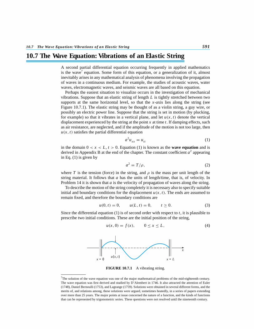
Perhaps the easiest situation to visualize occurs in the investigation of mechanicalvibrations. Suppose that an elastic string of length L is tightly stretched between twosupports at the same horizontal level, so that the x-axis lies along the string (seeFigure 10.7.1). The elastic string may be thought of as a violin string, a guy wire, orpossibly an electric power line. Suppose that the string is set in motion (by plucking,for example) so that it vibrates in a vertical plane, and let u(x, t) denote the verticaldisplacement experienced by the string at the point x at time t . If damping effects, suchas air resistance, are neglected, and if the amplitude of the motion is not too large, thenu(x, t) satisfies the partial differential equation
a2uxx = utt (1)
in the domain 0 < x < L , t > 0. Equation (1) is known as the wave equation and isderived in Appendix B at the end of the chapter. The constant coefficient a2 appearingin Eq. (1) is given by
a2 = T/ρ, (2)
where T is the tension (force) in the string, and ρ is the mass per unit length of thestring material. It follows that a has the units of length/time, that is, of velocity. InProblem 14 it is shown that a is the velocity of propagation of waves along the string.
To describe the motion of the string completely it is necessary also to specify suitableinitial and boundary conditions for the displacement u(x, t). The ends are assumed toremain fixed, and therefore the boundary conditions are
u(0, t) = 0, u(L , t) = 0, t ≥ 0. (3)
Since the differential equation (1) is of second order with respect to t , it is plausible toprescribe two initial conditions. These are the initial position of the string,
u(x, 0) = f (x), 0 ≤ x ≤ L , (4)
x
u(x, t)x = 0 x = L
FIGURE 10.7.1 A vibrating string.
7The solution of the wave equation was one of the major mathematical problems of the mid-eighteenth century.The wave equation was first derived and studied by D’Alembert in 1746. It also attracted the attention of Euler(1748), Daniel Bernoulli (1753), and Lagrange (1759). Solutions were obtained in several different forms, and themerits of, and relations among, these solutions were argued, sometimes heatedly, in a series of papers extendingover more than 25 years. The major points at issue concerned the nature of a function, and the kinds of functionsthat can be represented by trigonometric series. These questions were not resolved until the nineteenth century.

592 Chapter 10. Partial Differential Equations and Fourier Series
and its initial velocity,
ut(x, 0) = g(x), 0 ≤ x ≤ L , (5)
where f and g are given functions. In order for Eqs. (3), (4), and (5) to be consistentit is also necessary to require that
f (0) = f (L) = 0, g(0) = g(L) = 0. (6)
The mathematical problem then is to determine the solution of the wave equation (1)that also satisfies the boundary conditions (3) and the initial conditions (4) and (5). Likethe heat conduction problem of Sections 10.5 and 10.6, this problem is an initial valueproblem in the time variable t , and a boundary value problem in the space variable x .Alternatively, it can be considered as a boundary value problem in the semi-infinite strip0 < x < L , t > 0 of the xt-plane (see Figure 10.7.2). One condition is imposed at eachpoint on the semi-infinite sides, and two are imposed at each point on the finite base.
It is important to realize that Eq. (1) governs a large number of other wave problemsbesides the transverse vibrations of an elastic string. For example, it is only necessaryto interpret the function u and the constant a appropriately to have problems dealingwith water waves in an ocean, acoustic or electromagnetic waves in the atmosphere,or elastic waves in a solid body. If more than one space dimension is significant, thenEq. (1) must be slightly generalized. The two-dimensional wave equation is
a2(uxx + uyy) = utt . (7)
This equation would arise, for example, if we considered the motion of a thin elasticsheet, such as a drumhead. Similarly, in three dimensions the wave equation is
a2(uxx + uyy + uzz) = utt . (8)
In connection with the latter two equations, the boundary and initial conditions mustalso be suitably generalized.
We now solve some typical boundary value problems involving the one-dimensionalwave equation.
t
x
x = L
u(0, t) = 0 u(L, t) = 0
u(x, 0) = f (x)ut(x, 0) = g(x)
a2uxx = utt
FIGURE 10.7.2 Boundary value problem for the wave equation.

10.7 The Wave Equation: Vibrations of an Elastic String 593
Elastic String with Nonzero Initial Displacement. First suppose that the string isdisturbed from its equilibrium position, and then released at time t = 0 with zerovelocity to vibrate freely. Then the vertical displacement u(x, t) must satisfy the waveequation (1),
a2uxx = utt , 0 < x < L , t > 0;the boundary conditions (3),
u(0, t) = 0, u(L , t) = 0, t ≥ 0;and the initial conditions
u(x, 0) = f (x), ut(x, 0) = 0, 0 ≤ x ≤ L , (9)
where f is a given function describing the configuration of the string at t = 0.The method of separation of variables can be used to obtain the solution of Eqs. (1),
(3), and (9). Assuming that
u(x, t) = X (x)T (t) (10)
and substituting for u in Eq. (1), we obtain
X ′′
X= 1
a2
T ′′
T= −λ, (11)
where λ is a separation constant. Thus we find that X (x) and T (t) satisfy the ordinarydifferential equations
X ′′ + λX = 0, (12)
T ′′ + a2λT = 0. (13)
Further, by substituting from Eq. (10) for u(x, t) in the boundary conditions (3) wefind that X (x) must satisfy the boundary conditions
X (0) = 0, X (L) = 0. (14)
Finally, by substituting from Eq. (10) into the second of the initial conditions (9), wealso find that T (t) must satisfy the initial condition
T ′(0) = 0. (15)
Our next task is to determine X (x), T (t), and λ by solving Eq. (12) subject to theboundary conditions (14) and Eq. (13) subject to the initial condition (15).
The problem of solving the differential equation (12) subject to the boundary condi-tions (14) is precisely the same problem that arose in Section 10.5 in connection withthe heat conduction equation. Thus we can use the results obtained there and at the endof Section 10.1: The problem (12) and (14) has nontrivial solutions if and only if λ isan eigenvalue,
λ = n2π2/L2, n = 1, 2, . . . , (16)
and X (x) is proportional to the corresponding eigenfunction sin(nπx/L).Using the values of λ given by Eq. (16) in Eq. (13), we obtain
T ′′ + n2π2a2
L2 T = 0. (17)
594 Chapter 10. Partial Differential Equations and Fourier Series
Therefore
T (t) = k1 cosnπat
L+ k2 sin
nπat
L, (18)
where k1 and k2 are arbitrary constants. The initial condition (15) requires that k2 = 0,so T (t) must be proportional to cos(nπat/L).
Thus the functions
un(x, t) = sinnπx
Lcos
nπat
L, n = 1, 2, . . . , (19)
satisfy the partial differential equation (1), the boundary conditions (3), and the sec-ond initial condition (9). These functions are the fundamental solutions for the givenproblem.
To satisfy the remaining (nonhomogeneous) initial condition (9) we will considera superposition of the fundamental solutions (19) with properly chosen coefficients.Thus we assume that u(x, t) has the form
u(x, t) =∞∑
n=1
cnun(x, t) =∞∑
n=1
cn sinnπx
Lcos
nπat
L, (20)
where the constants cn remain to be chosen. The initial condition u(x, 0) = f (x)requires that
u(x, 0) =∞∑
n=1
cn sinnπx
L= f (x). (21)
Consequently, the coefficients cn must be the coefficients in the Fourier sine series ofperiod 2L for f ; hence
cn = 2
L
∫ L
0f (x) sin
nπx
Ldx, n = 1, 2, . . . . (22)
Thus the formal solution of the problem of Eqs. (1), (3), and (9) is given by Eq. (20)with the coefficients calculated from Eq. (22).
For a fixed value of n the expression sin(nπx/L) cos(nπat/L) in Eq. (19) is periodicin time t with the period 2L/na; it therefore represents a vibratory motion of the stringhaving this period, or having the frequency nπa/L . The quantities λa = nπa/L forn = 1, 2, . . . are the natural frequencies of the string, that is, the frequencies at whichthe string will freely vibrate. The factor sin(nπx/L) represents the displacement patternoccurring in the string when it is executing vibrations of the given frequency. Eachdisplacement pattern is called a natural mode of vibration and is periodic in the spacevariable x ; the spatial period 2L/n is called the wavelength of the mode of frequencynπa/L . Thus the eigenvalues n2π2/L2 of the problem (12), (14) are proportional tothe squares of the natural frequencies, and the eigenfunctions sin(nπx/L) give thenatural modes. The first three natural modes are sketched in Figure 10.7.3. The totalmotion of the string, given by the function u(x, t) of Eq. (20), is thus a combinationof the natural modes of vibration, and is also a periodic function of time with period2L/a.

10.7 The Wave Equation: Vibrations of an Elastic String 595
u
x
u
x
u
xL
L L
1 11
–1–1 –1
(a) (b) (c)
FIGURE 10.7.3 First three fundamental modes of vibration of an elastic string. (a) Frequency= πa/L , wavelength = 2L; (b) frequency = 2πa/L , wavelength = L; (c) frequency = 3πa/L ,wavelength = 2L/3.
E X A M P L E
1
Consider a vibrating string of length L = 30 that satisfies the wave equation
4uxx = utt , 0 < x < 30, t > 0 (23)
Assume that the ends of the string are fixed, and that the string is set in motion with noinitial velocity from the initial position
u(x, 0) = f (x) ={
x/10, 0 ≤ x ≤ 10,(30 − x)/20, 10 < x ≤ 30.
(24)
Find the displacement u(x, t) of the string and describe its motion through one period.The solution is given by Eq. (20) with a = 2 and L = 30, that is,
u(x, t) =∞∑
n=1
cn sinnπx
30cos
2nπ t
30, (25)
where cn is calculated from Eq. (22). Substituting from Eq. (24) into Eq. (22), weobtain
cn = 2
30
∫ 10
0
x
10sin
nπx
30dx + 2
30
∫ 30
10
30 − x
20sin
nπx
30dx . (26)
By evaluating the integrals in Eq. (26), we find that
cn = 9
n2π2 sinnπ
3, n = 1, 2, . . . . (27)
The solution (25), (27) gives the displacement of the string at any point x at any time t .The motion is periodic in time with period 30, so it is sufficient to analyze the solutionfor 0 ≤ t ≤ 30.
The best way to visualize the solution is by a computer animation showing thedynamic behavior of the vibrating string. Here we indicate the motion of the string inFigures 10.7.4, 10.7.5, and 10.7.6. Plots of u versus x for t = 0, 4, 7.5, 11, and 15are shown in Figure 10.7.4. Observe that the maximum initial displacement is positiveand occurs at x = 10, while at t = 15, a half period later, the maximum displacementis negative and occurs at x = 20. The string then retraces its motion and returns toits original configuration at t = 30. Figure 10.7.5 shows the behavior of the pointsx = 10, 15, and 20 by plots of u versus t for these fixed values of x . The plots confirmthat the motion is indeed periodic with period 30. Observe also that each interior point

596 Chapter 10. Partial Differential Equations and Fourier Series
on the string is motionless for one-third of each period. Figure 10.7.6 shows a three-dimensional plot of u versus both x and t , from which the overall nature of the solutionis apparent. Of course, the curves in Figures 10.7.4 and 10.7.5 lie on the surface shownin Figure 10.7.6.
x2 4 6 8 10 12 14 16 18 20 22 24 26 28 30
1
0.8
0.6
0.4
0.2
–0.2
–0.4
–0.6
–0.8
–1
u
t = 0
t = 4
t = 7.5
t = 11t = 15
FIGURE 10.7.4 Plots of u versus x for fixed values of t for the string in Example 1.
30 60
1
0.8
0.6
0.4
0.2
–0.2
–0.4
–0.6
–0.8
–1
t
u
50 40 20 10
x = 10
x = 15
x = 20
FIGURE 10.7.5 Plots of u versus t for fixed values of x for the string in Example 1.
Justification of the Solution. As in the heat conduction problem considered earlier,Eq. (20) with the coefficients cn given by Eq. (22) is only a formal solution of Eqs. (1),(3), and (9). To ascertain whether Eq. (20) actually represents the solution of the givenproblem requires some further investigation. As in the heat conduction problem, it istempting to try to show this directly by substituting Eq. (20) for u(x, t) in Eqs. (1), (3),and (9). However, on formally computing uxx , for example, we obtain
uxx(x, t) = −∞∑
n=1
cn
(nπ
L
)2sin
nπx
Lcos
nπat
L;

10.7 The Wave Equation: Vibrations of an Elastic String 597
30
25
20
2040
6080
15
10
5
1
–1
x
t
u
FIGURE 10.7.6 Plot of u versus x and t for the string in Example 1.
due to the presence of the n2 factor in the numerator this series may not converge. Thiswould not necessarily mean that the series (20) for u(x, t) is incorrect, but only that theseries (20) cannot be used to calculate uxx and utt . A basic difference between solutionsof the wave equation and those of the heat conduction equation is that the latter containnegative exponential terms that approach zero very rapidly with increasing n, whichensures the convergence of the series solution and its derivatives. In contrast, seriessolutions of the wave equation contain only oscillatory terms that do not decay withincreasing n.
However, there is an alternative way to establish the validity of Eq. (20) indirectly. Atthe same time we will gain additional information about the structure of the solution.First we will show that Eq. (20) is equivalent to
u(x, t) = 12 [h(x − at)+ h(x + at)], (28)
where h is the function obtained by extending the initial data f into (−L , 0) as an oddfunction, and to other values of x as a periodic function of period 2L . That is,
h(x) ={
f (x), 0 ≤ x ≤ L ,− f (−x), −L < x < 0; (29)
h(x + 2L) = h(x).
To establish Eq. (28) note that h has the Fourier series
h(x) =∞∑
n=1
cn sinnπx
L. (30)
Then, using the trigonometric identities for the sine of a sum or difference, we obtain
h(x − at) =∞∑
n=1
cn
(sin
nπx
Lcos
nπat
L− cos
nπx
Lsin
nπat
L
),
h(x + at) =∞∑
n=1
cn
(sin
nπx
Lcos
nπat
L+ cos
nπx
Lsin
nπat
L
),
598 Chapter 10. Partial Differential Equations and Fourier Series
and Eq. (28) follows immediately upon adding the last two equations. From Eq. (28)we see that u(x, t) is continuous for 0 < x < L , t > 0 provided that h is continuouson the interval (−∞,∞). This requires that f be continuous on the original interval[0, L]. Similarly, u is twice continuously differentiable with respect to either variablein 0 < x < L , t > 0, provided that h is twice continuously differentiable on (−∞,∞).This requires that f ′ and f ′′ be continuous on [0, L]. Furthermore, since h′′ is the oddextension of f ′′, we must also have f ′′(0) = f ′′(L) = 0. However, since h′ is the evenextension of f ′, no further conditions are required on f ′. Provided that these conditionsare met, uxx and utt can be computed from Eq. (28), and it is an elementary exerciseto show that these derivatives satisfy the wave equation. Some of the details of theargument just indicated are given in Problems 20 and 21.
If some of the continuity requirements stated in the last paragraph are not met, then uis not differentiable at some points in the semi-infinite strip 0 < x < L , t > 0, and thusis a solution of the wave equation only in a somewhat restricted sense. An importantphysical consequence of this observation is that if there are any discontinuities presentin the initial data f , then they will be preserved in the solution u(x, t) for all time.In contrast, in heat conduction problems initial discontinuities are instantly smoothedout (Section 10.6). Suppose that the initial displacement f has a jump discontinuityat x = x0, 0 ≤ x0 ≤ L . Since h is a periodic extension of f , the same discontinuity ispresent in h(ξ) at ξ = x0 + 2nL and at ξ = −x0 + 2nL , where n is any integer. Thush(x − at) is discontinuous when x − at = x0 + 2nL , or when x − at = −x0 + 2nL .For a fixed x in [0, L] the discontinuity that was originally at x0 will reappear inh(x − at) at the times t = (x ± x0 − 2nL)/a. Similarly, h(x + at) is discontinuous atthe point x at the times t = (−x ± x0 + 2mL)/a, where m is any integer. If we referto Eq. (28), it then follows that the solution u(x, t) is also discontinuous at the givenpoint x at these times. Since the physical problem is posed for t > 0, only those valuesof m and n yielding positive values of t are of interest.
General Problem for the Elastic String. Let us modify the problem considered pre-viously by supposing that the string is set in motion from its equilibrium positionwith a given velocity. Then the vertical displacement u(x, t) must satisfy the waveequation (1),
a2uxx = utt , 0 < x < L , t > 0;the boundary conditions (3),
u(0, t) = 0, u(L , t) = 0, t ≥ 0;and the initial conditions
u(x, 0) = 0, ut(x, 0) = g(x), 0 ≤ x ≤ L , (31)
where g(x) is the initial velocity at the point x of the string.The solution of this new problem can be obtained by following the procedure de-
scribed above for the problem (1), (3), and (9). Upon separating variables, we find thatthe problem for X (x) is exactly the same as before. Thus, once again λ = n2π2/L2
and X (x) is proportional to sin(nπx/L). The differential equation for T (t) is againEq. (17), but the associated initial condition is now
T (0) = 0. (32)
10.7 The Wave Equation: Vibrations of an Elastic String 599
corresponding to the first of the initial conditions (31). The general solution of Eq. (17)is given by Eq. (18), but now the initial condition (32) requires that k1 = 0. ThereforeT (t) is now proportional to sin(nπat/L) and the fundamental solutions for the problem(1), (3), and (31) are
un(x, t) = sinnπx
Lsin
nπat
L, n = 1, 2, 3, . . . . (33)
Each of the functions un(x, t) satisfies the wave equation (1), the boundary conditions(3), and the first of the initial conditions (31). The main consequence of using the initialconditions (31) rather than (9) is that the time-dependent factor in un(x, t) involves asine rather than a cosine.
To satisfy the remaining (nonhomogeneous) initial condition we assume that u(x, t)can be expressed as a linear combination of the fundamental solutions (33), that is,
u(x, t) =∞∑
n=1
knun(x, t) =∞∑
n=1
kn sinnπx
Lsin
nπat
L. (34)
To determine the values of the coefficients kn we differentiate Eq. (34) with respectto t , set t = 0, and use the second initial condition (31); this gives the equation
ut (x, 0) =∞∑
n=1
nπa
Lkn sin
nπx
L= g(x). (35)
Hence the quantities (nπa/L)kn are the coefficients in the Fourier sine series of period2L for g; therefore
nπa
Lkn = 2
L
∫ L
0g(x) sin
nπx
Ldx, n = 1, 2, . . . . (36)
Thus Eq. (34), with the coefficients given by Eq. (36), constitutes a formal solutionto the problem of Eqs. (1), (3), and (31). The validity of this formal solution canbe established by arguments similar to those previously indicated for the solution ofEqs. (1), (3), and (9).
Finally, we turn to the problem consisting of the wave equation (1), the boundaryconditions (3), and the general initial conditions (4), (5):
u(x, 0) = f (x), ut(x, 0) = g(x), 0 < x < L , (37)
where f (x) and g(x) are the given initial position and velocity, respectively, of thestring. Although this problem can be solved by separating variables, as in the casesdiscussed previously, it is important to note that it can also be solved simply by addingtogether the two solutions that we obtained above. To show that this is true, let v(x, t)be the solution of the problem (1), (3), and (9), and let w(x, t) be the solution of theproblem (1), (3), and (31). Thus v(x, t) is given by Eqs. (20) and (22), while w(x, t) isgiven by Eqs. (34) and (36). Now let u(x, t) = v(x, t)+ w(x, t); what problem doesu(x, t) satisfy? First, observe that
a2uxx − utt = (a2vxx − vt t)+ (a2wxx − wt t ) = 0 + 0 = 0, (38)
so u(x, t) satisfies the wave equation (1). Next, we have
u(0, t) = v(0, t)+ w(0, t) = 0 + 0 = 0, u(L , t) = v(L , t)+ w(L , t) = 0 + 0 = 0,
(39)

600 Chapter 10. Partial Differential Equations and Fourier Series
so u(x, t) also satisfies the boundary conditions (3). Finally, we have
u(x, 0) = v(x, 0)+ w(x, 0) = f (x)+ 0 = f (x) (40)
and
ut(x, 0) = vt (x, 0)+ wt (x, 0) = 0 + g(x) = g(x). (41)
Thus u(x, t) satisfies the general initial conditions (37).We can restate the result we have just obtained in the following way. To solve the wave
equation with the general initial conditions (37) you can solve instead the somewhatsimpler problems with the initial conditions (9) and (31), respectively, and then addtogether the two solutions. This is another use of the principle of superposition.
PROBLEMS Consider an elastic string of length L whose ends are held fixed. The string is set in motionwith no initial velocity from an initial position u(x, 0) = f (x). In each of Problems 1 through 4carry out the following steps. Let L = 10 and a = 1 in parts (b) through (d).
(a) Find the displacement u(x, t) for the given initial position f (x).(b) Plot u(x, t) versus x for 0 ≤ x ≤ 10 and for several values of t between t = 0 and t = 20.(c) Plot u(x, t) versus t for 0 ≤ t ≤ 20 and for several values of x .(d) Construct an animation of the solution in time for at least one period.(e) Describe the motion of the string in a few sentences.
� 1. f (x) ={
2x/L , 0 ≤ x ≤ L/2,2(L − x)/L , L/2 < x ≤ L
� 2. f (x) =
4x/L , 0 ≤ x ≤ L/4,1, L/4 < x < 3L/4,4(L − x)/L , 3L/4 ≤ x ≤ L
� 3. f (x) = 8x(L − x)2/L3
� 4. f (x) ={
1, L/2 − 1 < x < L/2 + 1 (L > 2),0, otherwise
Consider an elastic string of length L whose ends are held fixed. The string is set in motion fromits equilibrium position with an initial velocity ut (x, 0) = g(x). In each of Problems 5 through8 carry out the following steps. Let L = 10 and a = 1 in parts (b) through (d).
(a) Find the displacement u(x, t) for the given g(x).(b) Plot u(x, t) versus x for 0 ≤ x ≤ 10 and for several values of t between t = 0 and t = 20.(c) Plot u(x, t) versus t for 0 ≤ t ≤ 20 and for several values of x .(d) Construct an animation of the solution in time for at least one period.(e) Describe the motion of the string in a few sentences.
� 5. g(x) ={
2x/L , 0 ≤ x ≤ L/2,2(L − x)/L , L/2 < x ≤ L
� 6. g(x) =
4x/L , 0 ≤ x ≤ L/4,1, L/4 < x < 3L/4,4(L − x)/L , 3L/4 ≤ x ≤ L
� 7. g(x) = 8x(L − x)2/L3
� 8. g(x) ={
1, L/2 − 1 < x < L/2 + 1 (L > 2),0, otherwise

10.7 The Wave Equation: Vibrations of an Elastic String 601
9. If an elastic string is free at one end, the boundary condition to be satisfied there is thatux = 0. Find the displacement u(x, t) in an elastic string of length L , fixed at x = 0 andfree at x = L , set in motion with no initial velocity from the initial position u(x, 0) = f (x),where f is a given function.Hint: Show that the fundamental solutions for this problem, satisfying all conditions exceptthe nonhomogeneous initial condition, are
un(x, t) = sin λn x cos λnat,
where λn = (2n − 1)π/2L , n = 1, 2, . . . . Compare this problem with Problem 15 of Sec-tion 10.6; pay particular attention to the extension of the initial data out of the originalinterval [0, L].
� 10. Consider an elastic string of length L . The end x = 0 is held fixed while the end x = Lis free; thus the boundary conditions are u(0, t) = 0 and ux (L , t) = 0. The string is set inmotion with no initial velocity from the initial position u(x, 0) = f (x), where
f (x) ={
1, L/2 − 1 < x < L/2 + 1 (L > 2),0, otherwise.
(a) Find the displacement u(x, t).(b) With L = 10 and a = 1 plot u versus x for 0 ≤ x ≤ 10 and for several values of t . Payparticular attention to values of t between 3 and 7. Observe how the initial disturbance isreflected at each end of the string.(c) With L = 10 and a = 1 plot u versus t for several values of x .(d) Construct an animation of the solution in time for at least one period.(e) Describe the motion of the string in a few sentences.
� 11. Suppose that the string in Problem 10 is started instead from the initial position f (x) =8x(L − x)2/L3. Follow the instructions in Problem 10 for this new problem.
12. Dimensionless variables can be introduced into the wave equation a2uxx = utt in thefollowing manner. Let s = x/L and show that the wave equation becomes
a2uss = L2utt .
Then show that L/a has the dimensions of time, and thus can be used as the unit on thetime scale. Finally, let τ = at/L and show that the wave equation then reduces to
uss = uττ.
Problems 13 and 14 indicate the form of the general solution of the wave equation and thephysical significance of the constant a.
13. Show that the wave equation
a2uxx = utt
can be reduced to the form uξη
= 0 by change of variables ξ = x − at , η = x + at . Showthat u(x, t) can be written as
u(x, t) = φ(x − at)+ ψ(x + at),
where φ and ψ are arbitrary functions.14. Plot the value of φ(x − at) for t = 0, 1/a, 2/a, and t0/a if φ(s) = sin s. Note that for
any t �= 0 the graph of y = φ(x − at) is the same as that of y = φ(x) when t = 0, butdisplaced a distance at in the positive x direction. Thus a represents the velocity at whicha disturbance moves along the string. What is the interpretation of φ(x + at)?
15. A steel wire 5 ft in length is stretched by a tensile force of 50 lb. The wire has a weight perunit length of 0.026 lb/ft.(a) Find the velocity of propagation of transverse waves in the wire.

602 Chapter 10. Partial Differential Equations and Fourier Series
(b) Find the natural frequencies of vibration.(c) If the tension in the wire is increased, how are the natural frequencies changed? Arethe natural modes also changed?
16. A vibrating string moving in an elastic medium satisfies the equation
a2uxx − α2u = utt ,
where α2 is proportional to the coefficient of elasticity of the medium. Suppose that thestring is fixed at the ends, and is released with no initial velocity from the initial positionu(x, 0) = f (x), 0 < x < L . Find the displacement u(x, t).
17. Consider the wave equation
a2uxx = utt
in an infinite one-dimensional medium subject to the initial conditions
u(x, 0) = f (x), ut (x, 0) = 0, −∞ < x < ∞.
(a) Using the form of the solution obtained in Problem 13, show that φ and ψ must satisfy
φ(x)+ ψ(x) = f (x),
−φ′(x)+ ψ ′(x) = 0.
(b) Solve the equations of part (a) for φ and ψ , and thereby show that
u(x, t) = 12 [ f (x − at)+ f (x + at)].
This form of the solution was obtained by D’Alembert in 1746.Hint: Note that the equation ψ ′(x) = φ′(x) is solved by choosing ψ(x) = φ(x)+ c.(c) Let
f (x) ={
2, −1 < x < 1,0, otherwise.
Show that
f (x − at) ={
2, −1 + at < x < 1 + at,0, otherwise.
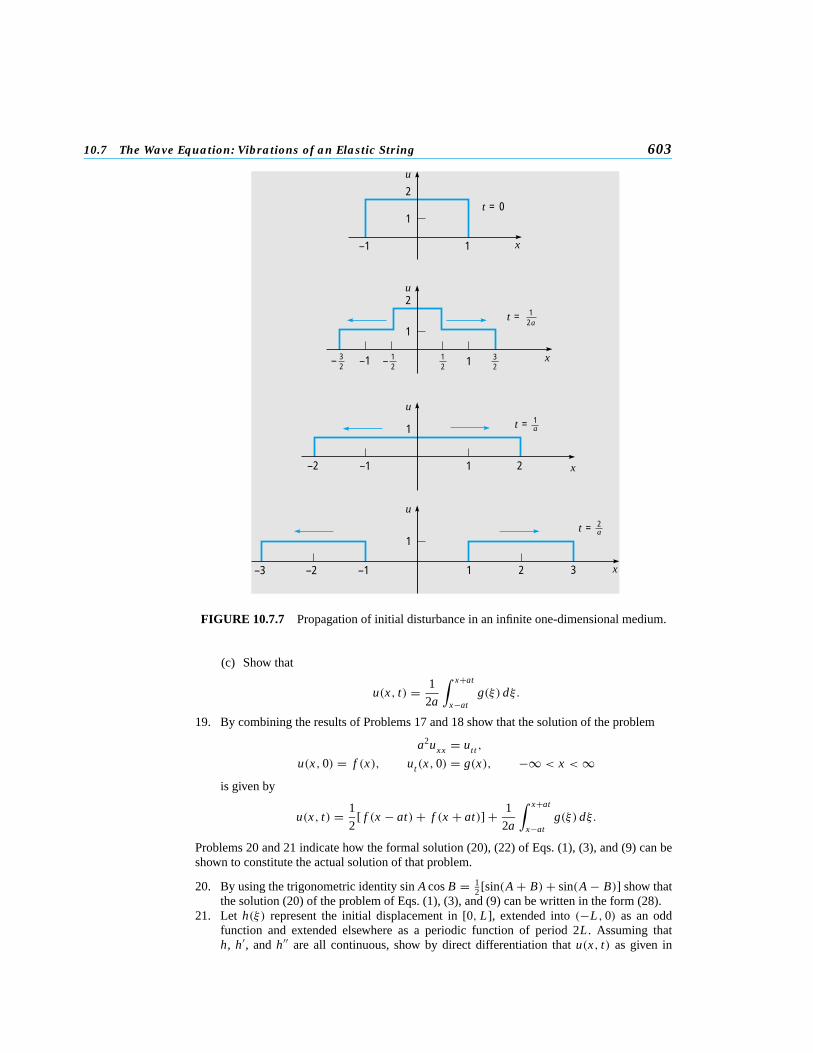
Also determine f (x + at).(d) Sketch the solution found in part (b) at t = 0, t = 1/2a, t = 1/a, and t = 2/a, obtain-ing the results shown in Figure 10.7.7. Observe that an initial displacement produces twowaves moving in opposite directions away from the original location; each wave consistsof one-half of the initial displacement.
18. Consider the wave equation
a2uxx = utt
in an infinite one-dimensional medium subject to the initial conditions
u(x, 0) = 0, ut (x, 0) = g(x), −∞ < x < ∞.
(a) Using the form of the solution obtained in Problem 13, show that
φ(x)+ ψ(x) = 0,
−aφ′(x)+ aψ ′(x) = g(x).
(b) Use the first equation of part (a) to show that ψ ′(x) = −φ′(x). Then use the secondequation to show that −2aφ′(x) = g(x), and therefore that
φ(x) = − 1
2a
∫ x
x0
g(ξ) dξ + φ(x0),
where x0 is arbitrary. Finally, determine ψ(x).
10.7 The Wave Equation: Vibrations of an Elastic String 603
x
u
x
x
x
u
u
u
2
1–1
1
–2–3
1
1
2
–1
–2 –1 1
1 2
2
3
–1
1
1
t = 0
t = 12a
– 32
12
32
– 12
t = 1a
t = 2a
FIGURE 10.7.7 Propagation of initial disturbance in an infinite one-dimensional medium.
(c) Show that
u(x, t) = 1
2a
∫ x+at
x−atg(ξ) dξ.
19. By combining the results of Problems 17 and 18 show that the solution of the problem
a2uxx = utt ,
u(x, 0) = f (x), ut (x, 0) = g(x), −∞ < x < ∞is given by
u(x, t) = 1
2[ f (x − at)+ f (x + at)] + 1
2a
∫ x+at
x−atg(ξ) dξ.
Problems 20 and 21 indicate how the formal solution (20), (22) of Eqs. (1), (3), and (9) can beshown to constitute the actual solution of that problem.
20. By using the trigonometric identity sin A cos B = 12 [sin(A + B)+ sin(A − B)] show that
the solution (20) of the problem of Eqs. (1), (3), and (9) can be written in the form (28).21. Let h(ξ) represent the initial displacement in [0, L], extended into (−L , 0) as an odd
function and extended elsewhere as a periodic function of period 2L . Assuming thath, h′, and h′′ are all continuous, show by direct differentiation that u(x, t) as given in
604 Chapter 10. Partial Differential Equations and Fourier Series
Eq. (28) satisfies the wave equation (1) and also the initial conditions (9). Note also thatsince Eq. (20) clearly satisfies the boundary conditions (3), the same is true of Eq. (28).Comparing Eq. (28) with the solution of the corresponding problem for the infinite string(Problem 17), we see that they have the same form provided that the initial data for thefinite string, defined originally only on the interval 0 ≤ x ≤ L , are extended in the givenmanner over the entire x-axis. If this is done, the solution for the infinite string is alsoapplicable to the finite one.
22. The motion of a circular elastic membrane, such as a drumhead, is governed by the two-dimensional wave equation in polar coordinates
urr + (1/r)ur + (1/r2)uθθ
= a−2utt .
Assuming that u(r, θ, t) = R(r)�(θ)T (t), find ordinary differential equations satisfied byR(r), �(θ), and T (t).
23. The total energy E(t) of the vibrating string is given as a function of time by
E(t) =∫ L
0
[12ρu2
t (x, t)+ 12 T u2
x (x, t)]
dx; (i)
the first term is the kinetic energy due to the motion of the string, and the second term isthe potential energy created by the displacement of the string away from its equilibriumposition.
For the displacement u(x, t) given by Eq. (20), that is, for the solution of the stringproblem with zero initial velocity, show that
E(t) = π2T
4L
∞∑n=1
n2c2n . (ii)
Note that the right side of Eq. (ii) does not depend on t . Thus the total energy E is aconstant, and therefore is conserved during the motion of the string.Hint: Use Parseval’s equation (Problem 37 of Section 10.4 and Problem 17 of Section10.3), and recall that a2 = T/ρ.
10.8 Laplace’s Equation
One of the most important of all partial differential equations occurring in appliedmathematics is that associated with the name of Laplace8: in two dimensions
uxx + uyy = 0, (1)
and in three dimensions
uxx + uyy + uzz = 0. (2)
For example, in a two-dimensional heat conduction problem, the temperature u(x, y, t)must satisfy the differential equation
α2(uxx + uyy) = ut , (3)
8Laplace’s equation is named for Pierre-Simon de Laplace, who, beginning in 1782, studied its solutions ex-tensively while investigating the gravitational attraction of arbitrary bodies in space. However, the equation firstappeared in 1752 in a paper by Euler on hydrodynamics.
10.8 Laplace’s Equation 605
where α2 is the thermal diffusivity. If a steady-state exists, u is a function of x and yonly, and the time derivative vanishes; in this case Eq. (3) reduces to Eq. (1). Similarly,for the steady-state heat conduction problem in three dimensions, the temperature mustsatisfy the three-dimensional form of Laplace’s equation. Equations (1) and (2) alsooccur in other branches of mathematical physics. In the consideration of electrostaticfields the electric potential function in a dielectric medium containing no electriccharges must satisfy either Eq. (1) or Eq. (2), depending on the number of spacedimensions involved. Similarly, the potential function of a particle in free space actedon only by gravitational forces satisfies the same equations. Consequently, Laplace’sequation is often referred to as the potential equation. Another example arises in thestudy of the steady (time-independent), two-dimensional, inviscid, irrotational motionof an incompressible fluid, which centers about two functions, known as the velocitypotential function and the stream function, both of which satisfy Eq. (1). In elasticitythe displacements that occur when a perfectly elastic bar is twisted are described interms of the so-called warping function, which also satisfies Eq. (1).
Since there is no time dependence in any of the problems mentioned previously,there are no initial conditions to be satisfied by the solutions of Eq. (1) or (2). Theymust, however, satisfy certain boundary conditions on the bounding curve or surface ofthe region in which the differential equation is to be solved. Since Laplace’s equationis of second order, it might be plausible to expect that two boundary conditions wouldbe required to determine the solution completely. This, however, is not the case. Recallthat in the heat conduction problem for the finite bar (Sections 10.5 and 10.6) it wasnecessary to prescribe one condition at each end of the bar, that is, one conditionat each point of the boundary. If we generalize this observation to multidimensionalproblems, it is then natural to prescribe one condition on the function u at each pointon the boundary of the region in which a solution of Eq. (1) or (2) is sought. The mostcommon boundary condition occurs when the value of u is specified at each boundarypoint; in terms of the heat conduction problem this corresponds to prescribing thetemperature on the boundary. In some problems the value of the derivative, or rate ofchange, of u in the direction normal to the boundary is specified instead; the conditionon the boundary of a thermally insulated body, for example, is of this type. It is entirelypossible for more complicated boundary conditions to occur; for example, u might beprescribed on part of the boundary, and its normal derivative specified on the remainder.The problem of finding a solution of Laplace’s equation that takes on given boundaryvalues is known as a Dirichlet problem, in honor of P. G. L. Dirichlet.9 In contrast, ifthe values of the normal derivative are prescribed on the boundary, the problem is saidto be a Neumann problem, in honor of K. G. Neumann.10 The Dirichlet and Neumannproblems are also known as the first and second boundary value problems of potentialtheory, respectively.
Physically, it is plausible to expect that the types of boundary conditions just men-tioned will be sufficient to determine the solution completely. Indeed, it is possible toestablish the existence and uniqueness of the solution of Laplace’s equation under the
9Peter Gustav Dirichlet (1805–1859) was a professor at Berlin and, after the death of Gauss, at Gottingen. In1829 he gave the first set of conditions sufficient to guarantee the convergence of a Fourier series. The definitionof function usually used today in elementary calculus is essentially the one given by Dirichlet in 1837. While heis best known for his work in analysis and differential equations, Dirichlet was also one of the leading numbertheorists of the nineteenth century.10Karl Gottfried Neumann (1832–1925), professor at Leipzig, made contributions to differential equations, integralequations, and complex variables.

606 Chapter 10. Partial Differential Equations and Fourier Series
boundary conditions mentioned, provided the shape of the boundary and the functionsappearing in the boundary conditions satisfy certain very mild requirements. However,the proofs of these theorems, and even their accurate statement, are beyond the scopeof the present book. Our only concern will be solving some typical problems by meansof separation of variables and Fourier series.
While the problems chosen as examples are capable of interesting physical interpre-tations (in terms of electrostatic potentials or steady-state temperature distributions, forinstance), our purpose here is primarily to point out some of the features that may occurduring their mathematical solution. It is also worth noting again that more complicatedproblems can sometimes be solved by expressing the solution as the sum of solutionsof several simpler problems (see Problems 3 and 4).
Dirichlet Problem for a Rectangle. Consider the mathematical problem of findingthe function u satisfying Laplace’s equation (1),
uxx + uyy = 0,
in the rectangle 0 < x < a, 0 < y < b, and also satisfying the boundary conditions
u(x, 0) = 0, u(x, b) = 0, 0 < x < a,(4)
u(0, y) = 0, u(a, y) = f (y), 0 ≤ y ≤ b,
where f is a given function on 0 ≤ y ≤ b (see Figure 10.8.1).To solve this problem we wish to construct a fundamental set of solutions satisfying
the partial differential equation and the homogeneous boundary conditions; then wewill superpose these solutions so as to satisfy the remaining boundary condition. Letus assume that
u(x, y) = X (x)Y (y) (5)
and substitute for u in Eq. (1). This yields
X ′′
X= −Y ′′
Y= λ,
where λ is the separation constant. Thus we obtain the two ordinary differentialequations
X ′′ − λX = 0, (6)
Y ′′ + λY = 0. (7)
y
x
b
a
u(0, y) = 0
u(x, b) = 0
u(a, y) = f (y)
u(x, 0) = 0
(a, b)
uxx + uyy = 0
FIGURE 10.8.1 Dirichlet problem for a rectangle.
10.8 Laplace’s Equation 607
If we now substitute for u from Eq. (5) in each of the homogeneous boundary conditions,we find that
X (0) = 0 (8)
and
Y (0) = 0, Y (b) = 0. (9)
We will first determine the solution of the differential equation (7) subject to theboundary conditions (9). However, this problem is essentially identical to one encoun-tered previously in Sections 10.1, 10.5, and 10.7. We conclude that there are nontrivialsolutions if and only if λ is an eigenvalue, namely,
λ = (nπ/b)2, n = 1, 2, . . . ; (10)
and Y (y) is proportional to the corresponding eigenfunction sin(nπy/b). Next, wesubstitute from Eq. (10) for λ in Eq. (6), and solve this equation subject to the boundarycondition (8). It is convenient to write the general solution of Eq. (6) as
X (x) = k1 cosh(nπx/b)+ k2 sinh(nπx/b), (11)
and the boundary condition (8) then requires that k1 = 0. Therefore X (x) must beproportional to sinh(nπx/b). Thus we obtain the fundamental solutions
un(x, y) = sinhnπx
bsin
nπy
b, n = 1, 2, . . . . (12)
These functions satisfy the differential equation (1) and all the homogeneous boundaryconditions for each value of n.
To satisfy the remaining nonhomogeneous boundary condition at x = a we assume,as usual, that we can represent the solution u(x, y) in the form
u(x, y) =∞∑
n=1
cnun(x, y) =∞∑
n=1
cn sinhnπx
bsin
nπy
b. (13)
The coefficients cn are determined by the boundary condition
u(a, y) =∞∑
n=1
cn sinhnπa
bsin
nπy
b= f (y). (14)
Therefore the quantities cn sinh(nπa/b) must be the coefficients in the Fourier sineseries of period 2b for f and are given by
cn sinhnπa
b= 2
b
∫ b
0f (y) sin
nπy
bdy. (15)
Thus the solution of the partial differential equation (1) satisfying the boundary condi-tions (4) is given by Eq. (13) with the coefficients cn computed from Eq. (15).
From Eqs. (13) and (15) we see that the solution contains the factorsinh(nπx/b)/ sinh(nπa/b). To estimate this quantity for large n we can use theapproximation sinh ξ ∼= eξ /2, and thereby obtain
sinh(nπx/b)
sinh(nπa/b)∼=
12 exp(nπx/b)12 exp(nπa/b)
= exp[−nπ(a − x)/b].
Thus this factor has the character of a negative exponential; consequently, the series(13) converges quite rapidly unless a − x is very small.

608 Chapter 10. Partial Differential Equations and Fourier Series
E X A M P L E
1
To illustrate these results, let a = 3, b = 2, and
f (y) ={
y, 0 ≤ y ≤ 1,2 − y, 1 ≤ y ≤ 2.
(16)
By evaluating cn from Eq. (15) we find that
cn = 8 sin(nπ/2)
n2π2 sinh(3nπ/2). (17)
Then u(x, y) is given by Eq. (13). Keeping 20 terms in the series we can plot u versusx and y, as shown in Figure 10.8.2. Alternatively, one can construct a contour plotshowing level curves of u(x, y); Figure 10.8.3 is such a plot, with an increment of 0.1between adjacent curves.
3y x
u
2
10.21
2 0.4
0.6
0.8
1.0
FIGURE 10.8.2 Plot of u versus x and y for Example 1.
1
x
2
y
u = 0
u = 0
u = 0u = 0.9
u = 0.7
u = 0.5
u = 0.4u = 0.2
u = 0.6
u = 0.8
u = 0.3
u = 0.1
321
FIGURE 10.8.3 Level curves of u(x, y) for Example 1.
10.8 Laplace’s Equation 609
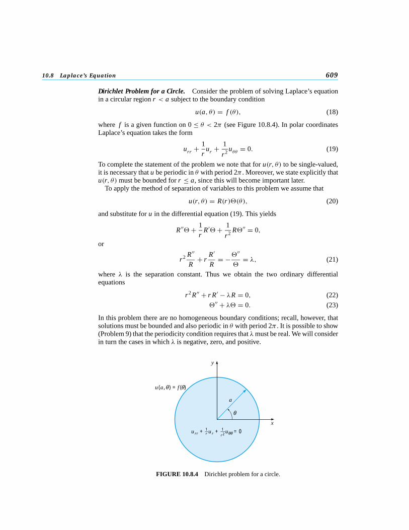
Dirichlet Problem for a Circle. Consider the problem of solving Laplace’s equationin a circular region r < a subject to the boundary condition
u(a, θ) = f (θ), (18)
where f is a given function on 0 ≤ θ < 2π (see Figure 10.8.4). In polar coordinatesLaplace’s equation takes the form
urr + 1
rur + 1
r2 uθθ
= 0. (19)
To complete the statement of the problem we note that for u(r, θ) to be single-valued,it is necessary that u be periodic in θ with period 2π . Moreover, we state explicitly thatu(r, θ) must be bounded for r ≤ a, since this will become important later.
To apply the method of separation of variables to this problem we assume that
u(r, θ) = R(r)�(θ), (20)
and substitute for u in the differential equation (19). This yields
R′′�+ 1
rR′�+ 1
r2 R�′′ = 0,
or
r2 R′′
R+ r
R′
R= −�
′′
�= λ, (21)
where λ is the separation constant. Thus we obtain the two ordinary differentialequations
r2 R′′ + r R′ − λR = 0, (22)
�′′ + λ� = 0. (23)
In this problem there are no homogeneous boundary conditions; recall, however, thatsolutions must be bounded and also periodic in θ with period 2π . It is possible to show(Problem 9) that the periodicity condition requires that λmust be real. We will considerin turn the cases in which λ is negative, zero, and positive.
y
x
a
θ
u(a, ) = f ( )θ θ
urr + ur + u = 01r
1r2 θθ
FIGURE 10.8.4 Dirichlet problem for a circle.
610 Chapter 10. Partial Differential Equations and Fourier Series
If λ < 0, let λ = −µ2, where µ > 0. Then Eq. (23) becomes �′′ − µ2� = 0, andconsequently
�(θ) = c1eµθ + c2e−µθ . (24)
Thus �(θ) can be periodic only if c1 = c2 = 0, and we conclude that λ cannot benegative.
If λ = 0, then Eq. (23) becomes �′′ = 0, and thus
�(θ) = c1 + c2θ. (25)
For �(θ) to be periodic we must have c2 = 0, so that �(θ) is a constant. Further, forλ = 0, Eq. (22) becomes
r2 R′′ + r R′ = 0. (26)
This equation is of the Euler type, and has the solution
R(r) = k1 + k2 ln r. (27)
The logarithmic term cannot be accepted if u(r, θ) is to remain bounded as r → 0; hencek2 = 0. Thus, corresponding to λ = 0, we conclude that u(r, θ) must be a constant,that is, proportional to the solution
u0(r, θ) = 1. (28)
Finally, if λ > 0, we let λ = µ2 where µ > 0. Then Eqs. (22) and (23) become
r2 R′′ + r R′ − µ2 R = 0 (29)
and
�′′ + µ2� = 0, (30)
respectively. Equation (29) is an Euler equation and has the solution
R(r) = k1rµ + k2r−µ, (31)
while Eq. (30) has the solution
�(θ) = c1 sinµθ + c2 cosµθ. (32)
In order that � be periodic with period 2π it is necessary that µ be a positive integern. With µ = n it follows that the solution r−µ in Eq. (31) must be discarded since itbecomes unbounded as r → 0. Consequently, k2 = 0 and the appropriate solutions ofEq. (19) are
un(r, θ) = rn cos nθ, vn(r, θ) = rn sin nθ, n = 1, 2, . . . . (33)
These functions, together with u0(r, θ) = 1, form a set of fundamental solutions forthe present problem.
In the usual way we now assume that u can be expressed as a linear combination ofthe fundamental solutions; that is,
u(r, θ) = c0
2+
∞∑n=1
rn(cn cos nθ + kn sin nθ). (34)
10.8 Laplace’s Equation 611
The boundary condition (18) then requires that
u(a, θ) = c0
2+
∞∑n=1
an(cn cos nθ + kn sin nθ) = f (θ) (35)
for 0 ≤ θ < 2π . The function f may be extended outside this interval so that it isperiodic with period 2π , and therefore has a Fourier series of the form (35). Sincethe extended function has period 2π , we may compute its Fourier coefficients byintegrating over any period of the function. In particular, it is convenient to use theoriginal interval (0, 2π); then
ancn = 1
π
∫ 2π
0f (θ) cos nθ dθ, n = 0, 1, 2, . . . ; (36)
ankn = 1
π
∫ 2π
0f (θ) sin nθ dθ, n = 1, 2, . . . . (37)
With this choice of the coefficients, Eq. (34) represents the solution of the boundaryvalue problem of Eqs. (18) and (19). Note that in this problem we needed both sineand cosine terms in the solution. This is because the boundary data were given on0 ≤ θ < 2π and have period 2π . As a consequence, the full Fourier series is required,rather than sine or cosine terms alone.
PROBLEMS
� 1. (a) Find the solution u(x, y) of Laplace’s equation in the rectangle 0 < x < a, 0 < y < b,also satisfying the boundary conditions
u(0, y) = 0, u(a, y) = 0, 0 < y < b,u(x, 0) = 0, u(x, b) = g(x), 0 ≤ x ≤ a.
(b) Find the solution if
g(x) ={
x, 0 ≤ x ≤ a/2,a − x, a/2 ≤ x ≤ a.
(c) For a = 3 and b = 1 plot u versus x for several values of y and also plot u versus y forseveral values of x .(d) Plot u versus both x and y in three dimensions. Also draw a contour plot showingseveral level curves of u(x, y) in the xy-plane.
2. Find the solution u(x, y) of Laplace’s equation in the rectangle 0 < x < a, 0 < y < b, alsosatisfying the boundary conditions
u(0, y) = 0, u(a, y) = 0, 0 < y < b,u(x, 0) = h(x), u(x, b) = 0, 0 ≤ x ≤ a.
� 3. (a) Find the solution u(x, y) of Laplace’s equation in the rectangle 0 < x < a, 0 < y < b,also satisfying the boundary conditions
u(0, y) = 0, u(a, y) = f (y), 0 < y < b,u(x, 0) = h(x), u(x, b) = 0, 0 ≤ x ≤ a.
Hint: Consider the possibility of adding the solutions of two problems, one with homo-geneous boundary conditions except for u(a, y) = f (y), and the other with homogeneousboundary conditions except for u(x, 0) = h(x).(b) Find the solution if h(x) = (x/a)2 and f (y) = 1 − (y/b).(c) Let a = 2 and b = 2. Plot the solution in several ways: u versus x , u versus y, u versusboth x and y, and a contour plot.
612 Chapter 10. Partial Differential Equations and Fourier Series
4. Show how to find the solution u(x, y) of Laplace’s equation in the rectangle 0 < x < a,0 < y < b, also satisfying the boundary conditions
u(0, y) = k(y), u(a, y) = f (y), 0 < y < b,u(x, 0) = h(x), u(x, b) = g(x), 0 ≤ x ≤ a.
Hint: See Problem 3.5. Find the solution u(r, θ) of Laplace’s equation
urr + (1/r)ur + (1/r2)uθθ
= 0
outside the circle r = a, also satisfying the boundary condition
u(a, θ) = f (θ), 0 ≤ θ < 2π,
on the circle. Assume that u(r, θ) is single-valued and bounded for r > a.� 6. (a) Find the solution u(r, θ) of Laplace’s equation in the semicircular region r < a,
0 < θ < π , also satisfying the boundary conditions
u(r, 0) = 0, u(r, π) = 0, 0 ≤ r < a,
u(a, θ) = f (θ), 0 ≤ θ ≤ π.
Assume that u is single-valued and bounded in the given region.(b) Find the solution if f (θ) = θ(π − θ).(c) Let a = 2 and plot the solution in several ways: u versus r , u versus θ , u versus bothr and θ , and a contour plot.
7. Find the solution u(r, θ) of Laplace’s equation in the circular sector 0 < r < a, 0 < θ < α,also satisfying the boundary conditions
u(r, 0) = 0, u(r, α) = 0, 0 ≤ r < a,
u(a, θ) = f (θ), 0 ≤ θ ≤ α.
Assume that u is single-valued and bounded in the sector.� 8. (a) Find the solution u(x, y) of Laplace’s equation in the semi-infinite strip 0 < x < a,
y > 0, also satisfying the boundary conditions
u(0, y) = 0, u(a, y) = 0, y > 0,
u(x, 0) = f (x), 0 ≤ x ≤ a
and the additional condition that u(x, y) → 0 as y → ∞.(b) Find the solution if f (x) = x(a − x).(c) Let a = 5. Find the smallest value of y0 for which u(x, y) ≤ 0.1 for all y ≥ y0.
9. Show that Eq. (23) has periodic solutions only if λ is real.Hint: Let λ = −µ2 where µ = ν + iσ with ν and σ real.
10. Consider the problem of finding a solution u(x, y) of Laplace’s equation in the rectangle0 < x < a, 0 < y < b, also satisfying the boundary conditions
ux (0, y) = 0, ux (a, y) = f (y), 0 < y < b,uy(x, 0) = 0, uy(x, b) = 0, 0 ≤ x ≤ a.
This is an example of a Neumann problem.(a) Show that Laplace’s equation and the homogeneous boundary conditions determinethe fundamental set of solutions
u0(x, y) = c0,
un(x, y) = cn cosh(nπx/b) cos(nπy/b), n = 1, 2, 3, . . . .
(b) By superposing the fundamental solutions of part (a), formally determine a function ualso satisfying the nonhomogeneous boundary condition ux (a, y) = f (y). Note that whenux (a, y) is calculated, the constant term in u(x, y) is eliminated, and there is no condition

10.8 Laplace’s Equation 613
from which to determine c0. Furthermore, it must be possible to express f by means of aFourier cosine series of period 2b, which does not have a constant term. This means that
∫ b
0f (y) dy = 0
is a necessary condition for the given problem to be solvable. Finally, note that c0 remainsarbitrary, and hence the solution is determined only up to this additive constant. This is aproperty of all Neumann problems.
11. Find a solution u(r, θ) of Laplace’s equation inside the circle r = a, also satisfying theboundary condition on the circle
ur (a, θ) = g(θ), 0 ≤ θ < 2π.
Note that this is a Neumann problem, and that its solution is determined only up to anarbitrary additive constant. State a necessary condition on g(θ) for this problem to besolvable by the method of separation of variables (see Problem 10).
� 12. (a) Find the solution u(x, y) of Laplace’s equation in the rectangle 0 < x < a, 0 < y < b,also satisfying the boundary conditions
u(0, y) = 0, u(a, y) = 0, 0 < y < b,uy(x, 0) = 0, u(x, b) = g(x), 0 ≤ x ≤ a.
Note that this is neither a Dirichlet nor a Neumann problem, but a mixed problem in whichu is prescribed on part of the boundary and its normal derivative on the rest.(b) Find the solution if
g(x) ={
x, 0 ≤ x ≤ a/2,a − x, a/2 ≤ x ≤ a.
(c) Let a = 3 and b = 1. By drawing suitable plots compare this solution with the solutionof Problem 1.
� 13. (a) Find the solution u(x, y) of Laplace’s equation in the rectangle 0 < x < a, 0 < y < b,also satisfying the boundary conditions
u(0, y) = 0, u(a, y) = f (y), 0 < y < b,u(x, 0) = 0, uy(x, b) = 0, 0 ≤ x ≤ a.
Hint: Eventually it will be necessary to expand f (y) in a series making use of the functionssin(πy/2b), sin(3πy/2b), sin(5πy/2b), . . . (see Problem 39 of Section 10.4).(b) Find the solution if f (y) = y(2b − y).(c) Let a = 3 and b = 2; plot the solution in several ways.
� 14. (a) Find the solution u(x, y) of Laplace’s equation in the rectangle 0 < x < a, 0 < y < b,also satisfying the boundary conditions
ux (0, y) = 0, ux (a, y) = 0, 0 < y < b,u(x, 0) = 0, u(x, b) = g(x), 0 ≤ x ≤ a.
(b) Find the solution if g(x) = 1 + x2(x − a)2.(c) Let a = 3 and b = 2; plot the solution in several ways.
15. By writing Laplace’s equation in cylindrical coordinates r , θ , and z and then assuming thatthe solution is axially symmetric (no dependence on θ ), we obtain the equation
urr + (1/r)ur + uzz = 0.
Assuming that u(r, z) = R(r)Z(z), show that R and Z satisfy the equations
r R′′ + R′ + λ2r R = 0, Z ′′ − λ2 Z = 0.
The equation for R is Bessel’s equation of order zero with independent variable λr .

614 Chapter 10. Partial Differential Equations and Fourier Series
A P P E N D I X
A
Derivation of the Heat Conduction Equation. In this section we derive the differ-ential equation that, to a first approximation at least, governs the conduction of heatin solids. It is important to understand that the mathematical analysis of a physicalsituation or process such as this ultimately rests on a foundation of empirical knowl-edge of the phenomenon involved. The mathematician must have a place to start, soto speak, and this place is furnished by experience. Consider a uniform rod insulatedon the lateral surfaces so that heat can flow only in the axial direction. It has beendemonstrated many times that if two parallel cross sections of the same area A anddifferent temperatures T1 and T2, respectively, are separated by a small distance d,an amount of heat per unit time will pass from the warmer section to the cooler one.Moreover, this amount of heat is proportional to the area A, the temperature difference| T2 − T1|, and inversely proportional to the separation distance d. Thus
Amount of heat per unit time = κA| T2 − T1|/d, (1)
where the positive proportionality factor κ is called the thermal conductivity anddepends primarily on the material11 of the rod. The relation (1) is often called Fourier’slaw of heat conduction. We repeat that Eq. (1) is an empirical, not a theoretical, resultand that it can be, and has often been, verified by careful experiment. It is the basis ofthe mathematical theory of heat conduction.
Now consider a straight rod of uniform cross section and homogeneous material,oriented so that the x-axis lies along the axis of the rod (see Figure 10.A.1). Let x = 0and x = L designate the ends of the bar.
x = x0 x = x0 + ∆x
H = – Auxκ H = Auxκ
x
FIGURE 10.A.1 Conduction of heat in an element of a rod.
We will assume that the sides of the bar are perfectly insulated so that there is nopassage of heat through them. We will also assume that the temperature u dependsonly on the axial position x and the time t , and not on the lateral coordinates y and z.In other words, we assume that the temperature remains constant on any cross sectionof the bar. This assumption is usually satisfactory when the lateral dimensions of therod are small compared to its length.
The differential equation governing the temperature in the bar is an expression of afundamental physical balance; the rate at which heat flows into any portion of the baris equal to the rate at which heat is absorbed in that portion of the bar. The terms in theequation are called the flux (flow) term and the absorption term, respectively.
We will first calculate the flux term. Consider an element of the bar lying betweenthe cross sections x = x0 and x = x0 +�x , where x0 is arbitrary and�x is small. The
11Actually, κ also depends on the temperature, but if the temperature range is not too great, it is satisfactory toassume that κ is independent of temperature.

Appendix A 615
instantaneous rate of heat transfer H(x0, t) from left to right across the cross sectionx = x0 is given by
H(x0) = − limd→0
κAu(x0 + d/2, t)− u(x0 − d/2, t)
d= −κAux(x0, t). (2)
The minus sign appears in this equation since there will be a positive flow of heat fromleft to right only if the temperature is greater to the left of x = x0 than to the right; inthis case ux(x0, t) is negative. In a similar manner, the rate at which heat passes fromleft to right through the cross section x = x0 +�x is given by
H(x0 +�x, t) = −κAux(x0 +�x, t). (3)
The net rate at which heat flows into the segment of the bar between x = x0 andx = x0 +�x is thus given by
Q = H(x0, t)− H(x0 +�x, t) = κA[ux(x0 +�x, t)− ux(x0, t)], (4)
and the amount of heat entering this bar element in time �t is
Q�t = κA[ux(x0 +�x, t)− ux(x0, t)]�t. (5)
Let us now calculate the absorption term. The average change in temperature �u,in the time interval �t , is proportional to the amount of heat Q�t introduced andinversely proportional to the mass �m of the element. Thus
�u = 1
s
Q�t
�m= Q�t
sρA�x, (6)
where the constant of proportionality s is known as the specific heat of the materialof the bar, and ρ is its density.12 The average temperature change �u in the barelement under consideration is the actual temperature change at some intermediatepoint x = x0 + θ �x , where 0 < θ < 1. Thus Eq. (6) can be written as
u(x0 + θ �x, t +�t)− u(x0 + θ �x, t) = Q�t
sρA�x, (7)
or as
Q�t = [u(x0 + θ �x, t +�t)− u(x0 + θ �x, t)]sρA�x . (8)
To balance the flux and absorption terms, we equate the two expressions for Q�t :
κA[ux(x0 +�x, t)− ux(x0, t)]�t
= sρA[u(x0 + θ �x, t +�t)− u(x0 + θ �x, t)]�x . (9)
On dividing Eq. (9) by �x �t and then letting �x → 0 and �t → 0, we obtain theheat conduction or diffusion equation
α2uxx = ut . (10)
The quantity α2 defined by
α2 = κ/ρs (11)
12The dependence of the density and specific heat on temperature is relatively small and will be neglected. Thusboth ρ and s will be considered as constants.

616 Chapter 10. Partial Differential Equations and Fourier Series
is called the thermal diffusivity, and is a parameter depending only on the material ofthe bar. The units ofα2 are (length)2/time. Typical values ofα2 are given in Table 10.5.1.
Several relatively simple conditions may be imposed at the ends of the bar. Forexample, the temperature at an end may be maintained at some constant value T . Thismight be accomplished by placing the end of the bar in thermal contact with somereservoir of sufficient size so that any heat that may flow between the bar and reservoirdoes not appreciably alter the temperature of the reservoir. At an end where this is donethe boundary condition is
u = T . (12)
Another simple boundary condition occurs if the end is insulated so that no heatpasses through it. Recalling the expression (2) for the amount of heat crossing anycross section of the bar, we conclude that the condition of insulation is that thisquantity vanish. Thus
ux = 0 (13)
is the boundary condition at an insulated end.A more general type of boundary condition occurs if the rate of flow of heat through
an end of the bar is proportional to the temperature there. Let us consider the end x = 0,where the rate of flow of heat from left to right is given by −κAux(0, t); see Eq. (2).Hence the rate of heat flow out of the bar (from right to left) at x = 0 is κAux(0, t).If this quantity is proportional to the temperature u(0, t), then we obtain the boundarycondition
ux(0, t)− h1u(0, t) = 0, t > 0, (14)
where h1 is a nonnegative constant of proportionality. Note that h1 = 0 corresponds toan insulated end, while h1 → ∞ corresponds to an end held at zero temperature.
If heat flow is taking place at the right end of the bar (x = L), then in a similar waywe obtain the boundary condition
ux(L , t)+ h2u(L , t) = 0, t > 0, (15)
where again h2 is a nonnegative constant of proportionality.Finally, to determine completely the flow of heat in the bar it is necessary to state
the temperature distribution at one fixed instant, usually taken as the initial time t = 0.This initial condition is of the form
u(x, 0) = f (x), 0 ≤ x ≤ L . (16)
The problem then is to determine the solution of the differential equation (10) subjectto one of the boundary conditions (12) to (15) at each end, and to the initial condition(16) at t = 0.
Several generalizations of the heat equation (10) also occur in practice. First, thebar material may be nonuniform and the cross section may not be constant along thelength of the bar. In this case, the parameters κ , ρ, s, and A may depend on the axialvariable x . Going back to Eq. (2) we see that the rate of heat transfer from left to rightacross the cross section at x = x0 is now given by
H(x0, t) = −κ(x0)A(x0)ux(x0, t) (17)
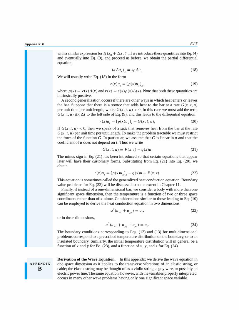
Appendix B 617
with a similar expression for H(x0 +�x, t). If we introduce these quantities into Eq. (4)and eventually into Eq. (9), and proceed as before, we obtain the partial differentialequation
(κAux)x = sρAut . (18)
We will usually write Eq. (18) in the form
r(x)ut = [p(x)ux ]x , (19)
where p(x) = κ(x)A(x) and r(x) = s(x)ρ(x)A(x). Note that both these quantities areintrinsically positive.
A second generalization occurs if there are other ways in which heat enters or leavesthe bar. Suppose that there is a source that adds heat to the bar at a rate G(x, t, u)per unit time per unit length, where G(x, t, u) > 0. In this case we must add the termG(x, t, u)�x �t to the left side of Eq. (9), and this leads to the differential equation
r(x)ut = [p(x)ux ]x + G(x, t, u). (20)
If G(x, t, u) < 0, then we speak of a sink that removes heat from the bar at the rateG(x, t, u) per unit time per unit length. To make the problem tractable we must restrictthe form of the function G. In particular, we assume that G is linear in u and that thecoefficient of u does not depend on t . Thus we write
G(x, t, u) = F(x, t)− q(x)u. (21)
The minus sign in Eq. (21) has been introduced so that certain equations that appearlater will have their customary forms. Substituting from Eq. (21) into Eq. (20), weobtain
r(x)ut = [p(x)ux ]x − q(x)u + F(x, t). (22)
This equation is sometimes called the generalized heat conduction equation. Boundaryvalue problems for Eq. (22) will be discussed to some extent in Chapter 11.
Finally, if instead of a one-dimensional bar, we consider a body with more than onesignificant space dimension, then the temperature is a function of two or three spacecoordinates rather than of x alone. Considerations similar to those leading to Eq. (10)can be employed to derive the heat conduction equation in two dimensions,
α2(uxx + uyy) = ut , (23)
or in three dimensions,
α2(uxx + uyy + uzz) = ut . (24)
The boundary conditions corresponding to Eqs. (12) and (13) for multidimensionalproblems correspond to a prescribed temperature distribution on the boundary, or to aninsulated boundary. Similarly, the initial temperature distribution will in general be afunction of x and y for Eq. (23), and a function of x , y, and z for Eq. (24).
A P P E N D I X
B
Derivation of the Wave Equation. In this appendix we derive the wave equation inone space dimension as it applies to the transverse vibrations of an elastic string, orcable; the elastic string may be thought of as a violin string, a guy wire, or possibly anelectric power line. The same equation, however, with the variables properly interpreted,occurs in many other wave problems having only one significant space variable.
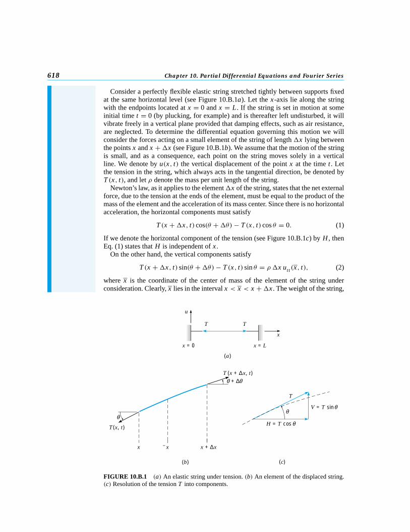
618 Chapter 10. Partial Differential Equations and Fourier Series
Consider a perfectly flexible elastic string stretched tightly between supports fixedat the same horizontal level (see Figure 10.B.1a). Let the x-axis lie along the stringwith the endpoints located at x = 0 and x = L . If the string is set in motion at someinitial time t = 0 (by plucking, for example) and is thereafter left undisturbed, it willvibrate freely in a vertical plane provided that damping effects, such as air resistance,are neglected. To determine the differential equation governing this motion we willconsider the forces acting on a small element of the string of length �x lying betweenthe points x and x +�x (see Figure 10.B.1b). We assume that the motion of the stringis small, and as a consequence, each point on the string moves solely in a verticalline. We denote by u(x, t) the vertical displacement of the point x at the time t . Letthe tension in the string, which always acts in the tangential direction, be denoted byT (x, t), and let ρ denote the mass per unit length of the string.
Newton’s law, as it applies to the element�x of the string, states that the net externalforce, due to the tension at the ends of the element, must be equal to the product of themass of the element and the acceleration of its mass center. Since there is no horizontalacceleration, the horizontal components must satisfy
T (x +�x, t) cos(θ +�θ)− T (x, t) cos θ = 0. (1)
If we denote the horizontal component of the tension (see Figure 10.B.1c) by H , thenEq. (1) states that H is independent of x .
On the other hand, the vertical components satisfy
T (x +�x, t) sin(θ +�θ)− T (x, t) sin θ = ρ �x utt(x, t), (2)
where x is the coordinate of the center of mass of the element of the string underconsideration. Clearly, x lies in the interval x < x < x +�x . The weight of the string,
u
x
TT
θθ
T
x x x + ∆x
(a)
(b) (c)
T (x + ∆x, t)θ θ+ ∆
V = T sinθ
H = T cos θT(x, t)
x = 0 x = L
FIGURE 10.B.1 (a) An elastic string under tension. (b) An element of the displaced string.(c) Resolution of the tension T into components.
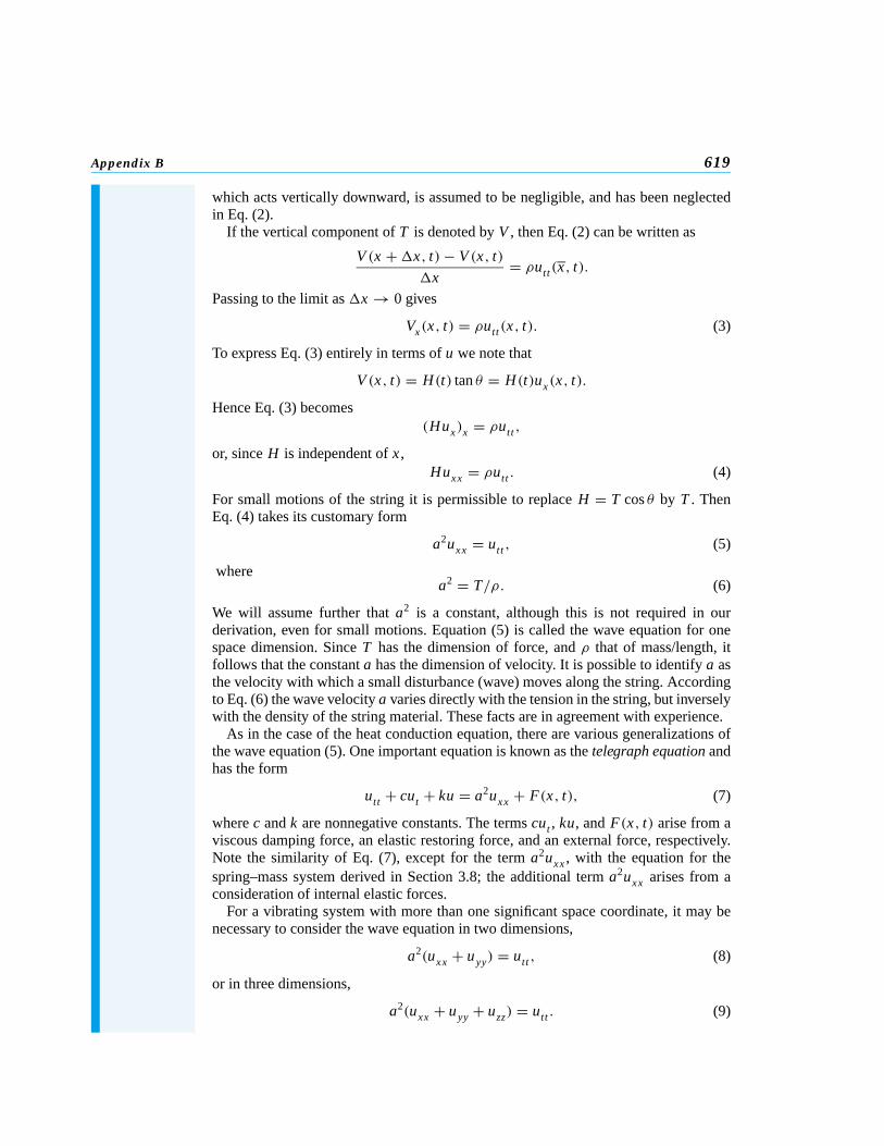
Appendix B 619
which acts vertically downward, is assumed to be negligible, and has been neglectedin Eq. (2).
If the vertical component of T is denoted by V , then Eq. (2) can be written as
V (x +�x, t)− V (x, t)
�x= ρutt(x, t).
Passing to the limit as �x → 0 gives
Vx(x, t) = ρutt(x, t). (3)
To express Eq. (3) entirely in terms of u we note that
V (x, t) = H(t) tan θ = H(t)ux(x, t).
Hence Eq. (3) becomes(Hux)x = ρutt ,
or, since H is independent of x ,Huxx = ρutt . (4)
For small motions of the string it is permissible to replace H = T cos θ by T . ThenEq. (4) takes its customary form
a2uxx = utt , (5)
wherea2 = T/ρ. (6)
We will assume further that a2 is a constant, although this is not required in ourderivation, even for small motions. Equation (5) is called the wave equation for onespace dimension. Since T has the dimension of force, and ρ that of mass/length, itfollows that the constant a has the dimension of velocity. It is possible to identify a asthe velocity with which a small disturbance (wave) moves along the string. Accordingto Eq. (6) the wave velocity a varies directly with the tension in the string, but inverselywith the density of the string material. These facts are in agreement with experience.
As in the case of the heat conduction equation, there are various generalizations ofthe wave equation (5). One important equation is known as the telegraph equation andhas the form
utt + cut + ku = a2uxx + F(x, t), (7)
where c and k are nonnegative constants. The terms cut , ku, and F(x, t) arise from aviscous damping force, an elastic restoring force, and an external force, respectively.Note the similarity of Eq. (7), except for the term a2uxx , with the equation for thespring–mass system derived in Section 3.8; the additional term a2uxx arises from aconsideration of internal elastic forces.
For a vibrating system with more than one significant space coordinate, it may benecessary to consider the wave equation in two dimensions,
a2(uxx + uyy) = utt , (8)
or in three dimensions,
a2(uxx + uyy + uzz) = utt . (9)
620 Chapter 10. Partial Differential Equations and Fourier Series
REFERENCES The following books contain additional information on Fourier series:
Buck, R. C., and Buck, E. F., Advanced Calculus (3rd ed.) (New York: McGraw-Hill, 1978).
Carslaw, H. S., Introduction to the Theory of Fourier’s Series and Integrals (3rd ed.) (Cambridge:Cambridge University Press, 1930; New York: Dover, 1952).
Courant, R., and John, F., Introduction to Calculus and Analysis (New York: Wiley-Interscience,1965; reprinted by Springer-Verlag, New York, 1989).
Kaplan, W., Advanced Calculus (4th ed.) (Reading, MA: Addison-Wesley, 1991).A brief biography of Fourier and an annotated copy of his 1807 paper are contained in:
Grattan-Guinness, I., Joseph Fourier 1768–1830 (Cambridge, MA: MIT Press, 1973).Useful references on partial differential equations and the method of separation of variables include the
following:
Churchill, R. V., and Brown, J. W., Fourier Series and Boundary Value Problems (5th ed.) (NewYork: McGraw-Hill, 1993).
Haberman, R., Elementary Applied Partial Differential Equations (3rd ed.) (Englewood Cliffs, NJ:Prentice Hall, 1998).
Pinsky, M. A., Partial Differential Equations and Boundary Value Problems with Applications (3rded.) (Boston: WCB/McGraw-Hill, 1998).
Powers, D. L., Boundary Value Problems (4th ed.) (San Diego: Academic Press, 1999).
Strauss, W. A., Partial Differential Equations, an Introduction (New York: Wiley, 1992).
Weinberger, H. F., A First Course in Partial Differential Equations (New York: Wiley, 1965; NewYork: Dover, 1995).

C H A P T E R
11
Boundary ValueProblems andSturm–LiouvilleTheory
As a result of separating variables in a partial differential equation in Chapter 10 werepeatedly encountered the differential equation
X ′′ + λX = 0, 0< x < L
with the boundary conditions
X (0) = 0, X (L) = 0.
This boundary value problem is the prototype of a large class of problems that are impor-tant in applied mathematics. These problems are known as Sturm–Liouville boundaryvalue problems. In this chapter we discuss the major properties of Sturm–Liouvilleproblems and their solutions; in the process we are able to generalize somewhat themethod of separation of variables for partial differential equations.
11.1 The Occurrence of Two-Point Boundary Value Problems
In Chapter 10 we described the method of separation of variables as a means of solvingcertain problems involving partial differential equations. The heat conduction problemconsisting of the partial differential equation
α2uxx = ut , 0< x < L , t > 0 (1)
621

622 Chapter 11. Boundary Value Problems and Sturm–Liouville Theory
subject to the boundary conditions
u(0, t) = 0, u(L , t) = 0, t > 0 (2)
and the initial condition
u(x,0) = f (x), 0 ≤ x ≤ L , (3)
is typical of the problems considered there. A crucial part of the process of solvingsuch problems is to find the eigenvalues and eigenfunctions of the differential equation
X ′′ + λX = 0, 0< x < L (4)
with the boundary conditions
X (0) = 0, X (L) = 0 (5)
or perhaps
X ′(0) = 0, X ′(L) = 0. (6)
The sine or cosine functions that result from solving Eq. (4) subject to the boundaryconditions (5) or (6) are used to expand the initial temperature distributionf (x) in aFourier series.
In this chapter we extend and generalize the results of Chapter 10. Our main goalis to show how the method of separation of variables can be used to solve problemssomewhat more general than that of Eqs. (1), (2), and (3). We are interested in threetypes of generalizations.
First, we wish to consider more general partial differential equations, for example,the equation
r(x)ut = [ p(x)ux ]x − q(x)u + F(x, t). (7)
This equation can arise, as indicated in Appendix A of Chapter 10, in the study of heatconduction in a bar of variable material properties in the presence of heat sources. Ifp andr are constants, and if the source termsqu andF are zero, then Eq. (7) reducesto Eq. (1). The partial differential equation (7) also occurs in the investigation of otherphenomena of a diffusive character.
A second generalization is to allow more general boundary conditions. In particular,we wish to consider boundary conditions of the form
ux(0, t)− h1u(0, t) = 0, ux(L , t)+ h2u(L , t) = 0. (8)
Such conditions occur when the rate of heat flow through an end of the bar is pro-portional to the temperature there. Usually,h1 andh2 are nonnegative constants, butin some cases they may be negative or depend ont . The boundary conditions (2) areobtained in the limit ash1 → ∞ and h2 → ∞. The other important limiting case,h1 = h2 = 0, gives the boundary conditions for insulated ends.
The final generalization that we discuss in this chapter concerns the geometry ofthe region in which the problem is posed. The results of Chapter 10 are adequate onlyfor a rather restricted class of problems, chiefly those in which the region of interestis rectangular or, in a few cases, circular. Later in this chapter we consider certainproblems posed in a few other geometrical regions.
Let us consider the equation
r(x)ut = [ p(x)ux ]x − q(x)u (9)

11.1 The Occurrence of Two-Point Boundary Value Problems 623
obtained by setting the termF(x, t) in Eq. (7) equal to zero. To separate the variableswe assume that
u(x, t) = X (x)T (t), (10)
and substitute foru in Eq. (9). We obtain
r(x)XT ′ = [ p(x)X ′]′T − q(x)XT (11)
or, upon dividing byr(x)XT ,
T ′
T= [ p(x)X ′]′
r(x)X− q(x)
r(x)= −λ. (12)
We have denoted the separation constant by−λ in anticipation of the fact that usuallyit will turn out to be real and negative. From Eq. (12) we obtain the following twoordinary differential equations forX andT :
[ p(x)X ′]′ − q(x)X + λr(x)X = 0, (13)
T ′ + λT = 0. (14)
If we substitute from Eq. (10) foru in Eqs. (8) and assume thath1 andh2 are constants,then we obtain the boundary conditions
X ′(0)− h1X (0) = 0, X ′(L)+ h2X (L) = 0. (15)
To proceed further we need to solve Eq. (13) subject to the boundary conditions (15).While this is a more general linear homogeneous two-point boundary value problemthan the problem consisting of the differential equation (4) and the boundary conditions(5) or (6), the solutions behave very much the same way. For every value ofλ, theproblem (13), (15) has the trivial solutionX (x) = 0. For certain values ofλ, calledeigenvalues, there are also other nontrivial solutions, calledeigenfunctions. Theseeigenfunctions form the basis for series solutions of a variety of problems in partialdifferential equations, such as the generalized heat conduction equation (9) subject tothe boundary conditions (8) and the initial condition (3).
In this chapter we discuss some of the properties of solutions of two-point boundaryvalue problems for second order linear equations. Sometimes we consider the generallinear homogeneous equation
P(x)y′′ + Q(x)y′ + R(x)y = 0, (16)
investigated in Chapter 3. However, for most purposes it is better to discuss equationsin which the first and second derivative terms are related as in Eq. (13). It is alwayspossible to transform the general equation (16) so that the derivative terms appear asin Eq. (13) (see Problem 11).
Boundary value problems with higher order differential equations can also occur;in them the number of boundary conditions must equal the order of the differentialequation. As a rule, the order of the differential equation is even, and half the boundaryconditions are given at each end of the interval. It is also possible for a single boundarycondition to involve values of the solution and/or its derivatives at both boundarypoints; for example,
y(0)− y(L) = 0. (17)

624 Chapter 11. Boundary Value Problems and Sturm–Liouville Theory
The following example involves one boundary condition of the form (15) and istherefore more complicated than the problems in Section 10.1.
E X A M P L E
1
Find the eigenvalues and the corresponding eigenfunctions of the boundary valueproblem
y′′ + λy = 0, (18)
y(0) = 0, y′(1)+ y(1) = 0. (19)
One place where this problem occurs is in the heat conduction problem in a bar of unitlength. The boundary condition atx = 0 corresponds to a zero temperature there. Theboundary condition atx = 1 corresponds to a rate of heat flow that is proportional tothe temperature there, and units are chosen so that the constant of proportionality is 1(see Appendix A of Chapter 10).
The solution of the differential equation may have one of several forms, dependingonλ, so it is necessary to consider several cases. First, ifλ = 0, the general solution ofthe differential equation is
y = c1x + c2. (20)
The two boundary conditions require that
c2 = 0, 2c1 + c2 = 0, (21)
respectively. The only solution of Eqs. (21) isc1 = c2 = 0, so the boundary valueproblem has no nontrivial solution in this case. Henceλ = 0 is not an eigenvalue.
If λ > 0, then the general solution of the differential equation (18) is
y = c1 sin√λ x + c2 cos
√λ x, (22)
where√λ > 0. The boundary condition atx = 0 requires thatc2 = 0; from the bound-
ary condition atx = 1 we then obtain the equation
c1(sin√λ+
√λ cos
√λ) = 0.
For a nontrivial solutiony we must havec1 = 0, and thusλ must satisfy
sin√λ+
√λ cos
√λ = 0. (23)
Note that ifλ is such that cos√λ = 0, then sin
√λ = 0, and Eq. (23) is not satisfied.
Hence we may assume that cos√λ = 0; dividing Eq. (23) by cos
√λ, we obtain
√λ = − tan
√λ. (24)
The solutions of Eq. (24) can be determined numerically. They can also be foundapproximately by sketching the graphs off (
√λ) = √
λ and g(√λ) = − tan
√λ for√
λ > 0 on the same set of axes, and identifying the points of intersection of thetwo curves (see Figure 11.1.1). The point
√λ = 0 is specifically excluded from this
argument because the solution (22) is valid only for√λ = 0. Despite the fact that the
curves intersect there,λ = 0 is not an eigenvalue, as we have already shown. The firstthree positive solutions of Eq. (24) are
√λ1
∼= 2.029,√λ2
∼= 4.913, and√λ3
∼= 7.979.As can be seen from Figure 11.1.1, the other roots are given with reasonable accuracy
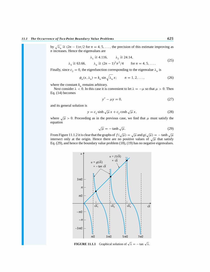
11.1 The Occurrence of Two-Point Boundary Value Problems 625
by√λn
∼= (2n − 1)π/2 for n = 4,5, . . . , the precision of this estimate improving asn increases. Hence the eigenvalues are
λ1∼= 4.116, λ2
∼= 24.14,(25)
λ3∼= 63.66, λn
∼= (2n − 1)2π2/4 for n = 4,5, . . . .
Finally, sincec2 = 0, the eigenfunction corresponding to the eigenvalueλn is
φn(x, λn) = kn sin√λn x; n = 1,2, . . . , (26)
where the constantkn remains arbitrary.Next considerλ < 0. In this case it is convenient to letλ = −µ so thatµ > 0. Then
Eq. (14) becomes
y′′ − µy = 0, (27)
and its general solution is
y = c1 sinhõ x + c2 cosh
õ x, (28)
where√µ > 0. Proceeding as in the previous case, we find thatµ must satisfy the
equation√µ = − tanh
õ. (29)
From Figure 11.1.2 it is clear that the graphs off (√µ) = √
µandg(√µ) = − tanh
õ
intersect only at the origin. Hence there are no positive values ofõ that satisfy
Eq. (29), and hence the boundary value problem (18), (19) has no negative eigenvalues.
u
3 /2π
3 /2π 5 /2π 7 /2π
π
/2π
/2π
/2–π
–π
3 /2π–
√ 1λ √ 2λ √ 3λ √λ
u = g(√ )λ= – tan √ λ
u = f (√ )λ= √ λ
FIGURE 11.1.1 Graphical solution of√λ = − tan
√λ.

626 Chapter 11. Boundary Value Problems and Sturm–Liouville Theory
u = f (√ )µ µ= √
µ√
u = g(√ )µ = –tanh√
u
1
–1
µ
1 2
FIGURE 11.1.2 Graphical solution of√µ = − tanh
õ.
Finally, it is necessary to consider the possibility thatλmay be complex. It is possibleto show by direct calculation that the problem (18), (19) has no complex eigenvalues.However, in Section 11.2 we consider in more detail a large class of problems thatincludes this example. One of the things we show there is that every problem in thisclass has only real eigenvalues. Therefore we omit the discussion of the nonexistence ofcomplex eigenvalues here. Thus we conclude that all the eigenvalues and eigenfunctionsof the problem (18), (19) are given by Eqs. (25) and (26).
PROBLEMS In each of Problems 1 through 6 state whether the given boundary value problem is homogeneousor nonhomogeneous.
1. y′′ + 4y = 0, y(−1) = 0, y(1) = 02. [(1 + x2)y′]′ + 4y = 0, y(0) = 0, y(1) = 13. y′′ + 4y = sinx, y(0) = 0, y(1) = 04. −y′′ + x2y = λy, y′(0)− y(0) = 0, y′(1)+ y(1) = 05. −[(1 + x2)y′]′ = λy + 1, y(−1) = 0, y(1) = 06. −y′′ = λ(1 + x2)y, y(0) = 0, y′(1)+ 3y(1) = 0
In each of Problems 7 through 10 determine the form of the eigenfunctions and the determinantalequation satisfied by the nonzero eigenvalues. Determine whetherλ = 0 is an eigenvalue, andfind approximate values forλ1 and λ2, the nonzero eigenvalues of smallest absolute value.Estimateλn for large values ofn. Assume that all eigenvalues are real.
7. y′′ + λy = 0,y(0) = 0, y(π)+ y′(π) = 0
8. y′′ + λy = 0,y′(0) = 0, y(1)+ y′(1) = 0
9. y′′ + λy = 0,y(0)− y′(0) = 0, y(1)+ y′(1) = 0
10. y′′ − λy = 0,y(0)+ y′(0) = 0, y(1) = 0
11. Consider the general linear homogeneous second order equation
P(x)y′′ + Q(x)y′ + R(x)y = 0. (i)
We seek an integrating factorµ(x) such that, upon multiplying Eq. (i) byµ(x), the resultingequation can be written in the form
[µ(x)P(x)y′]′ + µ(x)R(x)y = 0. (ii)
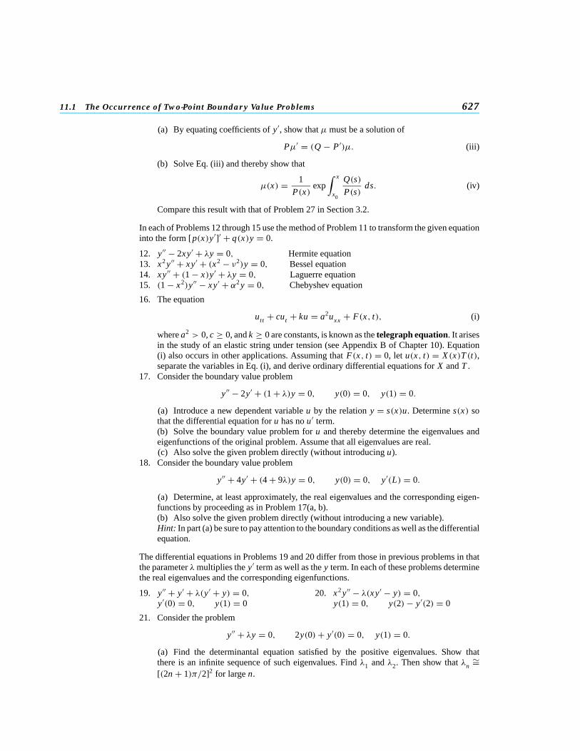
11.1 The Occurrence of Two-Point Boundary Value Problems 627
(a) By equating coefficients ofy′, show thatµ must be a solution of
Pµ′ = (Q − P ′)µ. (iii)
(b) Solve Eq. (iii) and thereby show that
µ(x) = 1
P(x)exp
∫ x
x0
Q(s)
P(s)ds. (iv)
Compare this result with that of Problem 27 in Section 3.2.
In each of Problems 12 through 15 use the method of Problem 11 to transform the given equationinto the form [p(x)y′]′ + q(x)y = 0.
12. y′′ − 2xy′ + λy = 0, Hermite equation13. x2y′′ + xy′ + (x2 − ν2)y = 0, Bessel equation14. xy′′ + (1 − x)y′ + λy = 0, Laguerre equation15. (1 − x2)y′′ − xy′ + α2y = 0, Chebyshev equation
16. The equation
utt + cut + ku = a2uxx + F(x, t), (i)
wherea2 > 0,c ≥ 0, andk ≥ 0 are constants, is known as thetelegraph equation. It arisesin the study of an elastic string under tension (see Appendix B of Chapter 10). Equation(i) also occurs in other applications. Assuming thatF(x, t) = 0, let u(x, t) = X (x)T (t),separate the variables in Eq. (i), and derive ordinary differential equations forX andT .
17. Consider the boundary value problem
y′′ − 2y′ + (1 + λ)y = 0, y(0) = 0, y(1) = 0.
(a) Introduce a new dependent variableu by the relationy = s(x)u. Determines(x) sothat the differential equation foru has nou′ term.(b) Solve the boundary value problem foru and thereby determine the eigenvalues andeigenfunctions of the original problem. Assume that all eigenvalues are real.(c) Also solve the given problem directly (without introducingu).
18. Consider the boundary value problem
y′′ + 4y′ + (4 + 9λ)y = 0, y(0) = 0, y′(L) = 0.
(a) Determine, at least approximately, the real eigenvalues and the corresponding eigen-functions by proceeding as in Problem 17(a, b).(b) Also solve the given problem directly (without introducing a new variable).Hint: In part (a) be sure to pay attention to the boundary conditions as well as the differentialequation.
The differential equations in Problems 19 and 20 differ from those in previous problems in thatthe parameterλmultiplies they′ term as well as they term. In each of these problems determinethe real eigenvalues and the corresponding eigenfunctions.
19. y′′ + y′ + λ(y′ + y) = 0,y′(0) = 0, y(1) = 0
20. x2y′′ − λ(xy′ − y) = 0,y(1) = 0, y(2)− y′(2) = 0
21. Consider the problem
y′′ + λy = 0, 2y(0)+ y′(0) = 0, y(1) = 0.
(a) Find the determinantal equation satisfied by the positive eigenvalues. Show thatthere is an infinite sequence of such eigenvalues. Findλ1 andλ2. Then show thatλn
∼=[(2n + 1)π/2]2 for largen.

628 Chapter 11. Boundary Value Problems and Sturm–Liouville Theory
(b) Find the determinantal equation satisfied by the negative eigenvalues. Show that thereis exactly one negative eigenvalue and find its value.
22. Consider the problem
y′′ + λy = 0, αy(0)+ y′(0) = 0, y(1) = 0,
whereα is a given constant.(a) Show that for all values ofα there is an infinite sequence of positive eigenvalues.(b) If α < 1, show that all (real) eigenvalues are positive. Show that the smallest eigenvalueapproaches zero asα approaches 1 from below.(c) Show thatλ = 0 is an eigenvalue only ifα = 1.(d) If α > 1, show that there is exactly one negative eigenvalue and that this eigenvaluedecreases asα increases.
23. Consider the problem
y′′ + λy = 0, y(0) = 0, y′(L) = 0.
Show that ifφm andφn are eigenfunctions, corresponding to the eigenvaluesλm andλn,respectively, withλm = λn , then
∫ L
0φm(x)φn(x) dx = 0.
Hint: Note that
φ′′m + λmφm = 0, φ′′
n + λnφn = 0.
Multiply the first of these equations byφn , the second byφm , and integrate from 0 toL,using integration by parts. Finally, subtract one equation from the other.
24. In this problem we consider a higher order eigenvalue problem. In the study of transversevibrations of a uniform elastic bar one is led to the differential equation
y iv − λy = 0,
wherey is the transverse displacement andλ = mω2/E I ; m is the mass per unit length ofthe rod,E is Young’s modulus,I is the moment of inertia of the cross section about anaxis through the centroid perpendicular to the plane of vibration, andω is the frequency ofvibration. Thus for a bar whose material and geometric properties are given, the eigenvaluesdetermine the natural frequencies of vibration. Boundary conditions at each end are usuallyone of the following types:
y = y′ = 0, clamped end,y = y′′ = 0, simply supported or hinged end,
y′′ = y′′′ = 0, free end.
For each of the following three cases find the form of the eigenfunctions and the equationsatisfied by the eigenvalues of this fourth order boundary value problem. Determineλ1 andλ2, the two eigenvalues of smallest magnitude. Assume that the eigenvalues are real andpositive.(a) y(0) = y′′(0) = 0, y(L) = y′′(L) = 0(b) y(0) = y′′(0) = 0, y(L) = y′(L) = 0(c) y(0) = y′(0) = 0, y′′(L) = y′′′(L) = 0 (cantilevered bar)
25. This problem illustrates that the eigenvalue parameter sometimes appears in the boundaryconditions as well as in the differential equation. Consider the longitudinal vibrations of auniform straight elastic bar of lengthL. It can be shown that the axial displacementu(x, t)satisfies the partial differential equation
(E/ρ)uxx = utt ; 0< x < L , t > 0, (i)

11.2 Sturm–Liouville Boundary Value Problems 629
whereE is Young’s modulus andρ is the mass per unit volume. If the endx = 0 is fixed,then the boundary condition there is
u(0, t) = 0, t > 0. (ii)
Suppose that the endx = L is rigidly attached to a massm but is otherwise unrestrained.We can obtain the boundary condition here by writing Newton’s law for the mass. Fromthe theory of elasticity it can be shown that the force exerted by the bar on the mass is givenby −E Aux (L , t). Hence the boundary condition is
E Aux (L , t)+ mutt (L , t) = 0, t > 0. (iii)
(a) Assume thatu(x, t) = X (x)T (t), and show thatX (x) andT (t) satisfy the differentialequations
X ′′ + λX = 0, (iv)
T ′′ + λ(E/ρ)T = 0. (v)
(b) Show that the boundary conditions are
X (0) = 0, X ′(L)− γλL X (L) = 0, (vi)
whereγ = m/ρAL is a dimensionless parameter that gives the ratio of the end mass to themass of the rod.Hint: Use the differential equation forT (t) in simplifying the boundary condition atx = L.(c) Determine the form of the eigenfunctions and the equation satisfied by the real eigen-values of Eqs. (iv) and (vi). Find the first two eigenvaluesλ1 andλ2 if γ = 0.5.
11.2 Sturm–Liouville Boundary Value Problems
We now consider two-point boundary value problems of the type obtained in Section11.1 by separating the variables in a heat conduction problem for a bar of variablematerial properties and with a source term proportional to the temperature. This kindof problem also occurs in many other applications.
These boundary value problems are commonly associated with the names of Sturmand Liouville.1 They consist of a differential equation of the form
[ p(x)y′]′ − q(x)y + λr(x)y = 0 (1)
on the interval 0< x < 1, together with the boundary conditions
a1y(0)+ a2y′(0) = 0, b1y(1)+ b2y′(1) = 0 (2)
1Charles-Franc¸ois Sturm (1803–1855) and Joseph Liouville (1809–1882), in a series of papers in 1836 and 1837,set forth many properties of the class of boundary value problems associated with their names, including theresults stated in Theorems 11.2.1 to 11.2.4. Sturm is also famous for a theorem on the number of real zeros of apolynomial, and in addition, did extensive work in physics and mechanics. Besides his own research in analysis,algebra, and number theory, Liouville was the founder, and for 39 years the editor, of the influentialJournal demathematiques pures et appliquees. One of his most important results was the proof (in 1844) of the existence oftranscendental numbers.

630 Chapter 11. Boundary Value Problems and Sturm–Liouville Theory
at the endpoints. It is often convenient to introduce the linear homogeneous differentialoperatorL defined by
L[y] = −[ p(x)y′]′ + q(x)y. (3)
Then the differential equation (1) can be written as
L[y] = λr(x)y. (4)
We assume that the functionsp, p′, q, andr are continuous on the interval 0≤ x ≤ 1and, further, thatp(x) > 0 andr(x) > 0 at all points in 0≤ x ≤ 1. These assumptionsare necessary to render the theory as simple as possible while retaining considerablegenerality. It turns out that these conditions are satisfied in many significant problems inmathematical physics. For example, the equationy′′ + λy = 0, which arose repeatedlyin the preceding chapter, is of the form (1) withp(x) = 1, q(x) = 0, andr(x) = 1.The boundary conditions (2) are said to beseparated; that is, each involves only oneof the boundary points. These are the most general separated boundary conditions thatare possible for a second order differential equation.
Before proceeding to establish some of the properties of the Sturm–Liouville problem(1), (2), it is necessary to derive an identity, known asLagrange’s identity, which isbasic to the study of linear boundary value problems. Letu andv be functions havingcontinuous second derivatives on the interval 0≤ x ≤ 1. Then2
∫ 1
0L[u]v dx =
∫ 1
0[−(pu′)′v + quv] dx .
Integrating the first term on the right side twice by parts, we obtain∫ 1
0L[u]v dx = −p(x)u′(x)v(x)
∣∣∣∣1
0
+ p(x)u(x)v′(x)∣∣∣∣1
0
+∫ 1
0[−u(pv′)′ + uqv] dx
= −p(x)[u′(x)v(x)− u(x)v′(x)]∣∣∣∣1
0
+∫ 1
0uL[v] dx .
Hence, on transposing the integral on the right side, we have∫ 1
0{L[u]v − uL[v]} dx = −p(x)[u′(x)v(x)− u(x)v′(x)]
∣∣∣∣1
0
, (5)
which is Lagrange’s identity.Now let us suppose that the functionsu andv in Eq. (5) also satisfy the boundary
conditions (2). Then, if we assume thata2 = 0 andb2 = 0, the right side of Eq. (5)becomes
−p(x)[u′(x)v(x)− u(x)v′(x)]∣∣∣10
= −p(1)[u′(1)v(1)− u(1)v′(1)] + p(0)[u′(0)v(0)− u(0)v′(0)]
= −p(1)
[−b1
b2
u(1)v(1)+ b1
b2
u(1)v(1)
]+ p(0)
[−a1
a2
u(0)v(0)+ a1
a2
u(0)v(0)
]
= 0.
2For brevity we sometimes use the notation∫ 1
0f dx rather than
∫ 1
0f (x) dx in this chapter.

11.2 Sturm–Liouville Boundary Value Problems 631
The same result holds if eithera2 or b2 is zero; the proof in this case is even simpler,and is left for you. Thus, if the differential operatorL is defined by Eq. (3), and if thefunctionsu andv satisfy the boundary conditions (2), Lagrange’s identity reduces to∫ 1
0{L[u]v − uL[v]} dx = 0. (6)
Let us now write Eq. (6) in a slightly different way. In Eq. (4) of Section 10.2 weintroduced the inner product(u, v) of two real-valued functionsu andv on a giveninterval; using the interval 0≤ x ≤ 1, we have
(u, v) =∫ 1
0u(x)v(x) dx . (7)
In this notation Eq. (6) becomes
(L[u], v)− (u, L[v]) = 0. (8)
In proving Theorem 11.2.1 below it is necessary to deal with complex-valued func-tions. By analogy with the definition in Section 7.2 for vectors, we define the innerproduct of two complex-valued functions on 0≤ x ≤ 1 as
(u, v) =∫ 1
0u(x)v(x) dx, (9)
wherev is the complex conjugate ofv. Clearly, Eq. (9) coincides with Eq. (7) ifu(x)andv(x) are real. It is important to know that Eq. (8) remains valid under the statedconditions ifu andv are complex-valued functions and if the inner product (9) is used.
To see this, one can start with the quantity∫ 1
0L[u]v dx and retrace the steps leading to
Eq. (6), making use of the fact thatp(x), q(x), a1, a2, b1, andb2 are all real quantities(see Problem 22).
We now consider some of the implications of Eq. (8) for the Sturm–Liouville bound-ary value problem (1), (2). We assume without proof3 that this problem actually haseigenvalues and eigenfunctions. In Theorems 11.2.1 to 11.2.4 below, we state severalof their important, but relatively elementary, properties. Each of these properties isillustrated by the basic Sturm–Liouville problem
y′′ + λy = 0, y(0) = 0, y(1) = 0, (10)
whose eigenvalues areλn = n2π2, with the corresponding eigenfunctionsφn(x) =sinnπx .
Theorem 11.2.1 All the eigenvalues of the Sturm–Liouville problem (1), (2) are real.
To prove this theorem let us suppose thatλ is a (possibly complex) eigenvalue of theproblem (1), (2) and thatφ is a corresponding eigenfunction, also possibly complex-valued. Let us writeλ = µ+ iν andφ(x) = U (x)+ iV (x), whereµ, ν, U (x), andV (x) are real. Then, if we letu = φ and alsov = φ in Eq. (8), we have
(L[φ], φ) = (φ, L[φ]). (11)
3The proof may be found, for example, in the references by Sagan (Chapter 5) or Birkhoff and Rota (Chapter 10).
632 Chapter 11. Boundary Value Problems and Sturm–Liouville Theory
However, we know thatL[φ] = λrφ, so Eq. (11) becomes
(λrφ, φ) = (φ, λrφ). (12)
Writing out Eq. (12) in full, using the definition (9) of the inner product, we obtain∫ 1
0λr(x)φ(x)φ(x) dx =
∫ 1
0φ(x)λr(x)φ(x) dx . (13)
Sincer(x) is real, Eq. (13) reduces to
(λ− λ)
∫ 1
0r(x)φ(x)φ(x) dx = 0,
or
(λ− λ)
∫ 1
0r(x)[U 2(x)+ V 2(x)] dx = 0. (14)
The integrand in Eq. (14) is nonnegative and not identically zero. Since the integrand isalso continuous, it follows that the integral is positive. Therefore, the factorλ − λ = 2iνmust be zero. Henceν = 0 andλ is real, so the theorem is proved.
An important consequence of Theorem 11.2.1 is that in finding eigenvalues andeigenfunctions of a Sturm–Liouville boundary value problem, one need look only forreal eigenvalues. Recall that this is what we did in Chapter 10. It is also possible toshow that the eigenfunctions of the boundary value problem (1), (2) are real. A proofis sketched in Problem 23.
Theorem 11.2.2 If φ1 andφ2 are two eigenfunctions of the Sturm–Liouville problem (1), (2) corre-sponding to eigenvaluesλ1 andλ2, respectively, and ifλ1 = λ2, then
∫ 1
0r(x)φ1(x)φ2(x) dx = 0. (15)
This theorem expresses the property oforthogonality of the eigenfunctions withrespect to the weight functionr . To prove the theorem we note thatφ1 andφ2 satisfythe differential equations
L[φ1] = λ1rφ1 (16)
and
L[φ2] = λ2rφ2, (17)
respectively. If we letu = φ1, v = φ2, and substitute forL[u] and L[v] in Eq. (8), weobtain
(λ1rφ1, φ2)− (φ1, λ2rφ2) = 0,
or, using Eq. (9),
λ1
∫ 1
0r(x)φ1(x)φ2(x) dx − λ2
∫ 1
0φ1(x)r(x)φ2(x) dx = 0.
11.2 Sturm–Liouville Boundary Value Problems 633
Becauseλ2, r(x), andφ2(x) are real, this equation becomes
(λ1 − λ2)
∫ 1
0r(x)φ1(x)φ2(x) dx = 0. (18)
Since by hypothesisλ1 = λ2, it follows thatφ1 andφ2 must satisfy Eq. (15), and thetheorem is proved.
Theorem 11.2.3 The eigenvalues of the Sturm–Liouville problem (1), (2) are all simple; that is, to eacheigenvalue there corresponds only one linearly independent eigenfunction. Further,the eigenvalues form an infinite sequence, and can be ordered according to increasingmagnitude so that
λ1 < λ2 < λ3 < · · · < λn < · · · .Moreover,λn → ∞ asn → ∞.
The proof of this theorem is somewhat more advanced than those of the two previoustheorems, and will be omitted. However, a proof that the eigenvalues are simple isindicated in Problem 20.
Again we note that all the properties stated in Theorems 11.2.1 to 11.2.3 are ex-emplified by the eigenvaluesλn = n2π2 and eigenfunctionsφn(x) = sinnπx of theexample problem (10). Clearly, the eigenvalues are real. The eigenfunctions satisfy theorthogonality relation
∫ 1
0φm(x)φn(x) dx =
∫ 1
0sinmπx sinnπx dx = 0, m = n, (19)
which was established in Section 10.2 by direct integration. Further, the eigenvalues canbe ordered so thatλ1 < λ2 < · · · , andλn → ∞ asn → ∞. Finally, to each eigenvaluethere corresponds a single linearly independent eigenfunction.
We will now assume that the eigenvalues of the Sturm–Liouville problem (1), (2)are ordered as indicated in Theorem 11.2.3. Associated with the eigenvalueλn is acorresponding eigenfunctionφn, determined up to a multiplicative constant. It is oftenconvenient to choose the arbitrary constant multiplying each eigenfunction so as tosatisfy the condition
∫ 1
0r(x)φ2
n(x) dx = 1, n = 1,2, . . . . (20)
Equation (20) is called a normalization condition, and eigenfunctions satisfying thiscondition are said to benormalized. Indeed, in this case, the eigenfunctions are saidto form anorthonormal set (with respect to the weight functionr ) since they alreadysatisfy the orthogonality relation (15). It is sometimes useful to combine Eqs. (15) and(20) into a single equation. To this end we introduce the symbolδmn, known as theKronecker (1823–1891) delta and defined by
δmn ={
0, if m = n,1, if m = n.
(21)
634 Chapter 11. Boundary Value Problems and Sturm–Liouville Theory
Making use of the Kronecker delta, we can write Eqs. (15) and (20) as∫ 1
0r(x)φm(x)φn(x) dx = δmn. (22)
E X A M P L E
1
Determine the normalized eigenfunctions of the problem (10):
y′′ + λy = 0, y(0) = 0, y(1) = 0.
The eigenvalues of this problem areλ1 = π2, λ2 = 4π2, . . . , λn = n2π2, . . . , andthe corresponding eigenfunctions arek1 sinπx , k2 sin 2πx, . . . , kn sinnπx, . . . , re-spectively. In this case the weight function isr(x) = 1. To satisfy Eq. (20) we mustchoosekn so that
∫ 1
0(kn sinnπx)2 dx = 1 (23)
for each value ofn. Since
k2n
∫ 1
0sin2 nπx dx = k2
n
∫ 1
0(1
2 − 12 cos 2nπx) dx = 1
2k2n,
Eq. (23) is satisfied ifkn is chosen to be√
2 for each value ofn. Hence the normalizedeigenfunctions of the given boundary value problem are
φn(x) =√
2 sinnπx, n = 1,2,3, . . . . (24)
E X A M P L E
2
Determine the normalized eigenfunctions of the problem
y′′ + λy = 0, y(0) = 0, y′(1)+ y(1) = 0. (25)
In Example 1 of Section 11.1 we found that the eigenvaluesλn satisfy the equation
sin√λn +
√λn cos
√λn = 0, (26)
and that the corresponding eigenfunctions are
φn(x) = kn sin√λn x, (27)
wherekn is arbitrary. We can determinekn from the normalization condition (20). Sincer(x) = 1 in this problem, we have∫ 1
0φ2
n(x) dx = k2n
∫ 1
0sin2
√λn x dx
= k2n
∫ 1
0
(12 − 1
2 cos 2√λn x
)dx = k2
n
(x
2− sin 2
√λn x
4√λn
) ∣∣∣∣1
0
= k2n
2√λn − sin 2
√λn
4√λn
= k2n
√λn − sin
√λn cos
√λn
2√λn
= k2n
1 + cos2√λn
2,
11.2 Sturm–Liouville Boundary Value Problems 635
where in the last step we have used Eq. (26). Hence, to normalize the eigenfunctionsφn we must choose
kn =(
2
1 + cos2√λn
)1/2
. (28)
The normalized eigenfunctions of the given problem are
φn(x) =√
2 sin√λn x
(1 + cos2√λn)
1/2 ; n = 1,2, . . . . (29)
We now turn to the question of expressing a given functionf as a series of eigen-functions of the Sturm–Liouville problem (1), (2). We have already seen examples ofsuch expansions in Sections 10.2 to 10.4. For example, it was shown there that iff iscontinuous and has a piecewise continuous derivative on 0≤ x ≤ 1, and satisfies theboundary conditionsf (0) = f (1) = 0, then f can be expanded in a Fourier sine seriesof the form
f (x) =∞∑
n=1
bn sinnπx . (30)
The functions sinnπx , n = 1,2, . . . , are precisely the eigenfunctions of the boundaryvalue problem (10). The coefficientsbn are given by
bn = 2∫ 1
0f (x) sinnπx dx (31)
and the series (30) converges for eachx in 0 ≤ x ≤ 1. In a similar way f can beexpanded in a Fourier cosine series using the eigenfunctions cosnπx , n = 0,1,2, . . . ,of the boundary value problemy′′ + λy = 0, y′(0) = 0, y′(1) = 0.
Now suppose that a given functionf , satisfying suitable conditions, can be expandedin an infinite series of eigenfunctions of the more general Sturm–Liouville problem(1), (2). If this can be done, then we have
f (x) =∞∑
n=1
cnφn(x), (32)
where the functionsφn(x) satisfy Eqs. (1), (2), and also the orthogonality condition(22). To compute the coefficients in the series (32) we multiply Eq. (32) byr(x)φm(x),wherem is a fixed positive integer, and integrate fromx = 0 to x = 1. Assuming thatthe series can be integrated term by term we obtain∫ 1
0r(x) f (x)φm(x) dx =
∞∑n=1
cn
∫ 1
0r(x)φm(x)φn(x) dx =
∞∑n=1
cnδmn. (33)
Hence, using the definition ofδmn, we have
cm =∫ 1
0r(x) f (x)φm(x) dx = ( f, rφm), m = 1,2, . . . . (34)
636 Chapter 11. Boundary Value Problems and Sturm–Liouville Theory
The coefficients in the series (32) have thus been formally determined. Equation (34)has the same structure as the Euler–Fourier formulas for the coefficients in a Fourierseries, and the eigenfunction series (32) also has convergence properties similar tothose of Fourier series. The following theorem is analogous to Theorem 10.3.1.
Theorem 11.2.4 Letφ1, φ2, . . . , φn, . . . be the normalized eigenfunctions of the Sturm–Liouville prob-lem (1), (2):
[ p(x)y′]′ − q(x)y + λr(x)y = 0,
a1y(0)+ a2y′(0) = 0, b1y(1)+ b2y′(1) = 0.
Let f and f ′ be piecewise continuous on 0≤ x ≤ 1. Then the series (32) whosecoefficientscm are given by Eq. (34) converges to [f (x+)+ f (x−)]/2 at each pointin the open interval 0< x < 1.
If f satisfies further conditions, then a stronger conclusion can be established.Suppose that, in addition to the hypotheses of Theorem 11.2.4, the functionf iscontinuous on 0≤ x ≤ 1. If a2 = 0 in the first of Eqs. (2) [so thatφn(0) = 0], thenassume thatf (0) = 0. Similarly, if b2 = 0 in the second of Eqs. (2), assume thatf (1) = 0. Otherwise no boundary conditions need be prescribed forf . Then the series(32) converges tof (x) at each point in the closed interval 0≤ x ≤ 1.
E X A M P L E
3
Expand the function
f (x) = x, 0 ≤ x ≤ 1 (35)
in terms of the normalized eigenfunctionsφn(x) of the problem (25).In Example 2 we found the normalized eigenfunctions to be
φn(x) = kn sin√λn x, (36)
wherekn is given by Eq. (28) andλn satisfies Eq. (26). To find the expansion forf interms of the eigenfunctionsφn we write
f (x) =∞∑
n=1
cnφn(x), (37)
where the coefficients are given by Eq. (34). Thus
cn =∫ 1
0f (x)φn(x) dx = kn
∫ 1
0x sin
√λn x dx .
Integrating by parts, we obtain
cn = kn
(sin√λn
λn
− cos√λn√
λn
)= kn
2 sin√λn
λn
,

11.2 Sturm–Liouville Boundary Value Problems 637
where we have used Eq. (26) in the last step. Upon substituting forkn from Eq. (28)we obtain
cn = 2√
2 sin√λn
λn(1 + cos2√λn)
1/2 . (38)
Thus
f (x) = 4∞∑
n=1
sin√λn sin
√λn x
λn(1 + cos2√λn)
. (39)
Observe that although the right side of Eq. (39) is a series of sines, it is not included inthe discussion of Fourier sine series in Section 10.4.
Self-adjoint Problems. Sturm–Liouville boundary value problems are of great im-portance in their own right, but they can also be viewed as belonging to a much moreextensive class of problems that have many of the same properties. For example, thereare many similarities between Sturm–Liouville problems and the algebraic system
Ax = λx, (40)
where then × n matrix A is real symmetric or Hermitian. Comparing the resultsmentioned in Section 7.3 with those of this section, we note that in both cases theeigenvalues are real and the eigenfunctions or eigenvectors form an orthogonal set.Further, the eigenfunctions or eigenvectors can be used as the basis for expressing anessentially arbitrary function or vector, respectively, as a sum. The most important dif-ference is that a matrix has only a finite number of eigenvalues and eigenvectors, whilea Sturm–Liouville problem has infinitely many. It is interesting and of fundamentalimportance in mathematics that these seemingly different problems—the matrix prob-lem (40) and the Sturm–Liouville problem (1), (2)—which arise in different ways, areactually part of a single underlying theory. This theory is usually referred to as linearoperator theory, and is part of the subject of functional analysis.
We now point out some ways in which Sturm–Liouville problems can be generalized,while still preserving the main results of Theorems 11.2.1 to 11.2.4—the existence of asequence of real eigenvalues tending to infinity, the orthogonality of the eigenfunctions,and the possibility of expressing an arbitrary function as a series of eigenfunctions. Inmaking these generalizations it is essential that the crucial relation (8) remain valid.
Let us consider the boundary value problem consisting of the differential equation
L[y] = λr(x)y, 0< x < 1, (41)
where
L[y] = Pn(x)dn y
dxn + · · · + P1(x)dy
dx+ P0(x)y, (42)
andn linear homogeneous boundary conditions at the endpoints. If Eq. (8) is valid forevery pair of sufficiently differentiable functions that satisfy the boundary conditions,then the given problem is said to beself-adjoint. It is important to observe that Eq. (8)involves restrictions on both the differential equation and the boundary conditions. Thedifferential operatorL must be such that the same operator appears in both terms of

638 Chapter 11. Boundary Value Problems and Sturm–Liouville Theory
Eq (8). This requires thatL be of even order. Further, a second order operator musthave the form (3), a fourth order operator must have the form
L[y] = [ p(x)y′′]′′ − [q(x)y′]′ + s(x)y, (43)
and higher order operators must have an analogous structure. In addition, the boundaryconditions must be such as to eliminate the boundary terms that arise during theintegration by parts used in deriving Eq. (8). For example, in a second order problemthis is true for the separated boundary conditions (2) and also in certain other cases,one of which is given in Example 4 below.
Let us suppose that we have a self-adjoint boundary value problem for Eq. (41),whereL[y] is given now by Eq. (43). We assume thatp, q, r , ands are continuous on0 ≤ x ≤ 1, and that the derivatives ofp andq indicated in Eq. (43) are also continuous.If in addition p(x) > 0 andr(x) > 0 for 0 ≤ x ≤ 1, then there is an infinite sequenceof real eigenvalues tending to+∞, the eigenfunctions are orthogonal with respectto the weight functionr , and an arbitrary function can be expressed as a series ofeigenfunctions. However, the eigenfunctions may not be simple in these more generalproblems.
We turn now to the relation between Sturm–Liouville problems and Fourier series.We have noted previously that Fourier sine and cosine series can be obtained byusing the eigenfunctions of certain Sturm–Liouville problems involving the differentialequationy′′ + λy = 0. This raises the question of whether we can obtain a full Fourierseries, including both sine and cosine terms, by choosing a suitable set of boundaryconditions. The answer is provided by the following example, which also serves toillustrate the occurrence of nonseparated boundary conditions.
E X A M P L E
4
Find the eigenvalues and eigenfunctions of the boundary value problem
y′′ + λy = 0, (44)
y(−L)− y(L) = 0, y′(−L)− y′(L) = 0. (45)
This is not a Sturm–Liouville problem because the boundary conditions are notseparated. The boundary conditions (45) are calledperiodic boundary conditionssince they require thaty and y′ assume the same values atx = L as atx = −L.Nevertheless, it is straightforward to show that the problem (44), (45) is self-adjoint. Asimple calculation establishes thatλ0 = 0 is an eigenvalue and that the correspondingeigenfunction isφ0(x) = 1. Further, there are additional eigenvaluesλ1 = (π/L)2,λ2 = (2π/L)2, . . . , λn = (nπ/L)2, . . . . To each of these nonzero eigenvalues therecorrespondtwo linearly independent eigenfunctions; for example, corresponding toλn are the two eigenfunctionsφn(x) = cos(nπx/L) andψn(x) = sin(nπx/L). Thisillustrates that the eigenvalues may not be simple when the boundary conditions arenot separated. Further, if we seek to expand a given functionf of period 2L in a seriesof eigenfunctions of the problem (44), (45), we obtain the series
f (x) = a0
2+
∞∑n=1
(an cos
nπx
L+ bn sin
nπx
L
),
which is just the Fourier series forf .

11.2 Sturm–Liouville Boundary Value Problems 639
We will not give further consideration to problems that have nonseparated boundaryconditions, nor will we deal with problems of higher than second order, except in afew problems. There is, however, one other kind of generalization that we do wishto discuss. That is the case in which the coefficientsp, q, andr in Eq. (1) do notquite satisfy the rather strict continuity and positivity requirements laid down at thebeginning of this section. Such problems are called singular Sturm–Liouville problems,and are the subject of Section 11.4.
PROBLEMS In each of Problems 1 through 5 determine the normalized eigenfunctions of the given problem.
1. y′′ + λy = 0, y(0) = 0, y′(1) = 02. y′′ + λy = 0, y′(0) = 0, y(1) = 03. y′′ + λy = 0, y′(0) = 0, y′(1) = 04. y′′ + λy = 0, y′(0) = 0, y′(1)+ y(1) = 0; see Section 11.1, Problem 8.5. y′′ − 2y′ + (1 + λ)y = 0, y(0) = 0, y(1) = 0; see Section 11.1, Problem 17.
In each of Problems 6 through 9 find the eigenfunction expansion∞∑
n=1anφn(x) of the given
function, using the normalized eigenfunctions of Problem 1.
6. f (x) = 1, 0 ≤ x ≤ 1 7. f (x) = x, 0 ≤ x ≤ 1
8. f (x) ={
1, 0 ≤ x < 12
0, 12 ≤ x ≤ 1
9. f (x) ={
2x, 0 ≤ x < 12
1, 12 ≤ x ≤ 1
In each of Problems 10 through 13 find the eigenfunction expansion∞∑
n=1anφn(x) of the given
function, using the normalized eigenfunctions of Problem 4.
10. f (x) = 1, 0 ≤ x ≤ 1 11. f (x) = x, 0 ≤ x ≤ 1
12. f (x) = 1 − x, 0 ≤ x ≤ 1 13. f (x) ={
1, 0 ≤ x < 12
0, 12 ≤ x ≤ 1
In each of Problems 14 through 18 determine whether the given boundary value problem isself-adjoint.
14. y′′ + y′ + 2y = 0, y(0) = 0, y(1) = 015. (1 + x2)y′′ + 2xy′ + y = 0, y′(0) = 0, y(1)+ 2y′(1) = 016. y′′ + y = λy, y(0)− y′(1) = 0, y′(0)− y(1) = 017. (1 + x2)y′′ + 2xy′ + y = λ(1 + x2)y, y(0)− y′(1) = 0, y′(0)+ 2y(1) = 018. y′′ + λy = 0, y(0) = 0, y(π)+ y′(π) = 0
19. Show that if the functionsu andv satisfy Eqs. (2), and eithera2 = 0 or b2 = 0, or both,then
p(x)[u′(x)v(x)− u(x)v′(x)]∣∣∣∣1
0
= 0.
20. In this problem we outline a proof of the first part of Theorem 11.2.3: that the eigenvaluesof the Sturm–Liouville problem (1), (2) are simple. For a givenλ suppose thatφ1 andφ2are two linearly independent eigenfunctions. Compute the WronskianW (φ1, φ2)(x) anduse the boundary conditions (2) to show thatW (φ1, φ2)(0) = 0. Then use Theorems 3.3.2and 3.3.3 to conclude thatφ1 andφ2 cannot be linearly independent as assumed.
21. Consider the Sturm–Liouville problem
− [ p(x)y′]′ + q(x)y = λr(x)y,
a1y(0)+ a2y′(0) = 0, b1y(1)+ b2y′(1) = 0,

640 Chapter 11. Boundary Value Problems and Sturm–Liouville Theory
wherep, q, andr satisfy the conditions stated in the text.(a) Show that ifλ is an eigenvalue andφ a corresponding eigenfunction, then
λ
∫ 1
0rφ2 dx =
∫ 1
0(pφ′2 + qφ2) dx + b1
b2
p(1)φ2(1)− a1
a2
p(0)φ2(0),
provided thata2 = 0 andb2 = 0. How must this result be modified ifa2 = 0 or b2 = 0?(b) Show that ifq(x) ≥ 0 and ifb1/b2 and−a1/a2 are nonnegative, then the eigenvalueλis nonnegative.(c) Under the conditions of part (b) show that the eigenvalueλ is strictly positive unlessq(x) = 0 for eachx in 0 ≤ x ≤ 1 and alsoa1 = b1 = 0.
22. Derive Eq. (8) using the inner product (9) and assuming thatu andv are complex-valuedfunctions.Hint: Consider the quantity
∫ 1
0L[u] v dx , split u andv into real and imaginary parts, and
proceed as in the text.23. In this problem we indicate a proof that the eigenfunctions of the Sturm–Liouville problem
(1), (2) are real.(a) Let λ be an eigenvalue andφ a corresponding eigenfunction. Letφ(x) = U(x)+iV (x), and show thatU andV are also eigenfunctions corresponding toλ.(b) Using Theorem 11.2.3, or the result of Problem 20, show thatU andV are linearlydependent.(c) Show thatφ must be real, apart from an arbitrary multiplicative constant that may becomplex.
24. Consider the problem
x2y′′ = λ(xy′ − y), y(1) = 0, y(2) = 0.
Note thatλ appears as a coefficient ofy′ as well as ofy itself. It is possible to extendthe definition of self-adjointness to this type of problem, and to show that this particularproblem is not self-adjoint. Show that the problem has eigenvalues, but that none of themis real. This illustrates that in general nonself-adjoint problems may have eigenvalues thatare not real.
Buckling of an Elastic Column. In an investigation of the buckling of a uniform elasticcolumn of lengthL by an axial loadP (Figure 11.2.1a) one is led to the differential equation
y iv + λy′′ = 0, 0< x < L . (i)
The parameterλ is equal toP/E I , whereE is Young’s modulus andI is the moment of inertia ofthe cross section about an axis through the centroid perpendicular to thexy-plane. The boundaryconditions atx = 0 andx = L depend on how the ends of the column are supported. Typicalboundary conditions are
y = y′ = 0, clamped end;y = y′′ = 0, simply supported (hinged) end.
The bar shown in Figure 11.2.1a is simply supported atx = 0 and clamped atx = L. It isdesired to determine the eigenvalues and eigenfunctions of Eq. (i) subject to suitable boundaryconditions. In particular, the smallest eigenvalueλ1 gives the load at which the column buckles,or can assume a curved equilibrium position, as shown in Figure 11.2.1b. The correspondingeigenfunction describes the configuration of the buckled column. Note that the differentialequation (i) does not fall within the theory discussed in this section. It is possible to show,however, that in each of the cases given here all the eigenvalues are real and positive. Problems25 and 26 deal with column buckling problems.
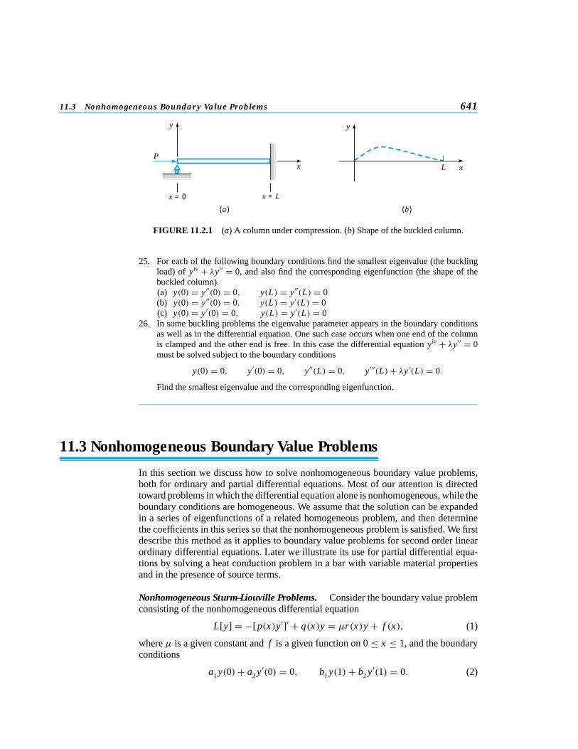
11.3 Nonhomogeneous Boundary Value Problems 641
y
x
y
P
x = 0 x = L
L
(a) (b)
x
FIGURE 11.2.1 (a) A column under compression. (b) Shape of the buckled column.
25. For each of the following boundary conditions find the smallest eigenvalue (the bucklingload) of y iv + λy′′ = 0, and also find the corresponding eigenfunction (the shape of thebuckled column).(a) y(0) = y′′(0) = 0, y(L) = y′′(L) = 0(b) y(0) = y′′(0) = 0, y(L) = y′(L) = 0(c) y(0) = y′(0) = 0, y(L) = y′(L) = 0
26. In some buckling problems the eigenvalue parameter appears in the boundary conditionsas well as in the differential equation. One such case occurs when one end of the columnis clamped and the other end is free. In this case the differential equationy iv + λy′′ = 0must be solved subject to the boundary conditions
y(0) = 0, y′(0) = 0, y′′(L) = 0, y′′′(L)+ λy′(L) = 0.
Find the smallest eigenvalue and the corresponding eigenfunction.
11.3 Nonhomogeneous Boundary Value Problems
In this section we discuss how to solve nonhomogeneous boundary value problems,both for ordinary and partial differential equations. Most of our attention is directedtoward problems in which the differential equation alone is nonhomogeneous, while theboundary conditions are homogeneous. We assume that the solution can be expandedin a series of eigenfunctions of a related homogeneous problem, and then determinethe coefficients in this series so that the nonhomogeneous problem is satisfied. We firstdescribe this method as it applies to boundary value problems for second order linearordinary differential equations. Later we illustrate its use for partial differential equa-tions by solving a heat conduction problem in a bar with variable material propertiesand in the presence of source terms.
Nonhomogeneous Sturm–Liouville Problems. Consider the boundary value problemconsisting of the nonhomogeneous differential equation
L[y] = −[ p(x)y′]′ + q(x)y = µr(x)y + f (x), (1)
whereµ is a given constant andf is a given function on 0≤ x ≤ 1, and the boundaryconditions
a1y(0)+ a2y′(0) = 0, b1y(1)+ b2y′(1) = 0. (2)
642 Chapter 11. Boundary Value Problems and Sturm–Liouville Theory
As in Section 11.2 we assume thatp, p′, q, andr are continuous on 0≤ x ≤ 1 andthat p(x) > 0 andr(x) > 0 there. We will solve the problem (1), (2) by making useof the eigenfunctions of the corresponding homogeneous problem consisting of thedifferential equation
L[y] = λr(x)y (3)
and the boundary conditions (2). Letλ1 < λ2 < · · · < λn < · · · be the eigenvaluesof this problem, and letφ1, φ2, . . . , φn, . . . be the corresponding normalized eigen-functions.
We now assume that the solutiony = φ(x) of the nonhomogeneous problem (1), (2)can be expressed as a series of the form
φ(x) =∞∑
n=1
bnφn(x). (4)
From Eq. (34) of Section 11.2 we know that
bn =∫ 1
0r(x)φ(x)φn(x) dx, n = 1,2, . . . . (5)
However, since we do not knowφ(x), we cannot use Eq. (5) to calculatebn. Instead, wewill try to determinebn so that the problem (1), (2) is satisfied, and then use Eq. (4) tofindφ(x). Note first thatφ as given by Eq. (4) always satisfies the boundary conditions(2) since eachφn does.
Now consider the differential equation thatφ must satisfy. This is just Eq. (1) withy replaced byφ:
L[φ](x) = µr(x)φ(x)+ f (x). (6)
We substitute the series (4) into the differential equation (6) and attempt to determinebn so that the differential equation is satisfied. The term on the left side of Eq. (6)becomes
L[φ](x) = L
[ ∞∑n=1
bnφn
](x) =
∞∑n=1
bn L[φn](x)
=∞∑
n=1
bnλnr(x)φn(x), (7)
where we have assumed that we can interchange the operations of summation anddifferentiation.
Note that the functionr appears in Eq. (7) and also in the termµr(x)φ(x) in Eq. (6).This suggests that we rewrite the nonhomogeneous term in Eq. (6) asr(x)[ f (x)/r(x)]so thatr(x) also appears as a multiplier in this term. If the functionf/r satisfies theconditions of Theorem 11.2.4, then
f (x)
r(x)=
∞∑n=1
cnφn(x), (8)
where, using Eq. (5) withφ replaced byf/r ,
cn =∫ 1
0r(x)
f (x)
r(x)φn(x) dx =
∫ 1
0f (x)φn(x) dx, n = 1,2, . . . . (9)
11.3 Nonhomogeneous Boundary Value Problems 643
Upon substituting forφ(x), L[φ](x), and f (x) in Eq. (6) from Eqs. (4), (7), and (8),respectively, we find that
∞∑n=1
bnλnr(x)φn(x) = µr(x)∞∑
n=1
bnφn(x)+ r(x)∞∑
n=1
cnφn(x).
After collecting terms and canceling the common nonzero factorr(x) we have
∞∑n=1
[(λn − µ)bn − cn
]φn(x) = 0. (10)
If Eq. (10) is to hold for eachx in the interval 0≤ x ≤ 1, then the coefficient ofφn(x)must be zero for eachn; see Problem 14 for a proof of this fact. Hence
(λn − µ)bn − cn = 0, n = 1,2, . . . . (11)
We must now distinguish two main cases, one of which also has two subcases.First suppose thatµ = λn for n = 1,2,3, . . . ; that is,µ is not equal to any eigenvalue
of the corresponding homogeneous problem. Then
bn = cn
λn − µ, n = 1,2,3, . . . , (12)
and
y = φ(x) =∞∑
n=1
cn
λn − µφn(x). (13)
Equation (13), withcn given by Eq. (9), is a formal solution of the nonhomogeneousboundary value problem (1), (2). Our argument does not prove that the series (13)converges. However, any solution of the boundary value problem (1), (2) clearly satisfiesthe conditions of Theorem 11.2.4; indeed, it satisfies the more stringent conditions givenin the paragraph following that theorem. Thus it is reasonable to expect that the series(13) does converge at each point, and this fact can be established provided, for example,that f is continuous.
Now suppose thatµ is equal to one of the eigenvalues of the corresponding homo-geneous problem, say,µ = λm ; then the situation is quite different. In this event, forn = m Eq. (11) has the form 0· bm − cm = 0. Again we must consider two cases.
If µ = λm and cm = 0, then it is impossible to solve Eq. (11) forbm , and thenonhomogeneous problem (1), (2) has no solution.
If µ = λm andcm = 0, then Eq. (11) is satisfied regardless of the value ofbm ; inother words,bm remains arbitrary. In this case the boundary value problem (1), (2)does have a solution, but it is not unique, since it contains an arbitrary multiple of theeigenfunctionφm .
Sincecm is given by Eq. (9), the conditioncm = 0 means that∫ 1
0f (x)φm(x) dx = 0. (14)
Thus, ifµ = λm , the nonhomogeneous boundary value problem (1), (2) can be solvedonly if f is orthogonal to the eigenfunction corresponding to the eigenvalueλm .
The results we have formally obtained are summarized in the following theorem.

644 Chapter 11. Boundary Value Problems and Sturm–Liouville Theory
Theorem 11.3.1 The nonhomogeneous boundary value problem (1), (2) has a unique solution for eachcontinuousf wheneverµ is different from all the eigenvalues of the correspondinghomogeneous problem; the solution is given by Eq. (13), and the series convergesfor eachx in 0 ≤ x ≤ 1. If µ is equal to an eigenvalueλm of the correspondinghomogeneous problem, then the nonhomogeneous boundary value problem has nosolution unlessf is orthogonal toφm ; that is, unless the condition (14) holds. In thatcase, the solution is not unique and contains an arbitrary multiple ofφm(x).
The main part of Theorem 11.3.1 is sometimes stated in the following way:
Theorem 11.3.2 For a given value ofµ, either the nonhomogeneous problem (1), (2) has a uniquesolution for each continuousf (if µ is not equal to any eigenvalueλm of the cor-responding homogeneous problem), or else the homogeneous problem (3), (2) has anontrivial solution (the eigenfunction corresponding toλm).
This latter form of the theorem is known as the Fredholm4 alternative theorem. Thisis one of the basic theorems of mathematical analysis and occurs in many differentcontexts. You may be familiar with it in connection with sets of linear algebraic equa-tions where the vanishing or nonvanishing of the determinant of coefficients replacesthe statements aboutµ andλm . See the discussion in Section 7.3.
E X A M P L E
1
Solve the boundary value problem
y′′ + 2y = −x, (15)
y(0) = 0, y(1)+ y′(1) = 0. (16)
This particular problem can be solved directly in an elementary way and has thesolution
y = sin√
2 x
sin√
2 + √2 cos
√2
− x
2. (17)
The method of solution described below illustrates the use of eigenfunction expan-sions, a method that can be employed in many problems not accessible by elementaryprocedures. To identify Eq. (15) with Eq. (1) it is helpful to write the former as
−y′′ = 2y + x . (18)
We seek the solution of the given problem as a series of normalized eigenfunctionsφn of the corresponding homogeneous problem
y′′ + λy = 0, y(0) = 0, y(1)+ y′(1) = 0. (19)
4The Swedish mathematician Erik Ivar Fredholm (1866–1927), professor at the University of Stockholm, estab-lished the modern theory of integral equations in a fundamental paper in 1903. Fredholm’s work emphasized thesimilarities between integral equations and systems of linear algebraic equations. There are also many interrelationsbetween differential and integral equations; for example, see Section 2.8 and Problem 21 of Section 6.6.
11.3 Nonhomogeneous Boundary Value Problems 645
These eigenfunctions were found in Example 2 of Section 11.2, and are
φn(x) = kn sin√λn x, (20)
where
kn =(
2
1 + cos2√λn
)1/2
(21)
andλn satisfies
sin√λn +
√λn cos
√λn = 0. (22)
Recall that in Example 1 of Section 11.1 we found that
λ1∼= 4.116, λ2
∼= 24.14,
λ3∼= 63.66, λn
∼= (2n − 1)2π2/4 for n = 4,5, . . . .
We assume thaty is given by Eq. (4),
y =∞∑
n=1
bnφn(x),
and it follows that the coefficientsbn are found from Eq. (12),
bn = cn
λn − 2,
where thecn are the expansion coefficients of the nonhomogeneous termf (x) = x inEq. (18) in terms of the eigenfunctionsφn. These coefficients were found in Example3 of Section 11.2, and are
cn = 2√
2 sin√λn
λn(1 + cos2√λn)
1/2 . (23)
Putting everything together, we finally obtain the solution
y = 4∞∑
n=1
sin√λn
λn(λn − 2)(1 + cos2√λn)
sin√λn x . (24)
While Eqs. (17) and (24) are quite different in appearance, they are actually twodifferent expressions for the same function. This follows from the uniqueness part ofTheorem 11.3.1 or 11.3.2 sinceλ = 2 is not an eigenvalue of the homogeneous problem(19). Alternatively, one can show the equivalence of Eqs. (17) and (24) by expandingthe right side of Eq. (17) in terms of the eigenfunctionsφn(x). For this problem it isfairly obvious that the formula (17) is more convenient than the series formula (24).However, we emphasize again that in other problems we may not be able to obtain thesolution except by series (or numerical) methods.
646 Chapter 11. Boundary Value Problems and Sturm–Liouville Theory
Nonhomogeneous Heat Conduction Problems. To show how eigenfunction expan-sions can be used to solve nonhomogeneous problems for partial differential equations,let us consider the generalized heat conduction equation
r(x)ut = [ p(x)ux ]x − q(x)u + F(x, t) (25)
with the boundary conditions
ux(0, t)− h1u(0, t) = 0, ux(1, t)+ h2u(1, t) = 0 (26)
and the initial condition
u(x,0) = f (x). (27)
This problem was previously discussed in Appendix A of Chapter 10 and in Section11.1. In the latter section we letu(x, t) = X (x)T (t) in the homogeneous equationobtained by settingF(x, t) = 0, and showed thatX (x) must be a solution of theboundary value problem
− [ p(x)X ′]′ + q(x)X = λr(x)X, (28)
X ′(0)− h1X (0) = 0, X ′(1)+ h2X (1) = 0. (29)
If we assume thatp, q, andr satisfy the proper continuity requirements and thatp(x)andr(x) are always positive, the problem (28), (29) is a Sturm–Liouville problem asdiscussed in Section 11.2. Thus we obtain a sequence of eigenvaluesλ1 < λ2 < · · · <λn < · · · and corresponding normalized eigenfunctionsφ1(x), φ2(x), . . . , φn(x), . . . .
We will solve the given nonhomogeneous boundary value problem (25) to (27) byassuming thatu(x, t) can be expressed as a series of eigenfunctions,
u(x, t) =∞∑
n=1
bn(t)φn(x), (30)
and then showing how to determine the coefficientsbn(t). The procedure is basicallythe same as that used in the problem (1), (2) considered earlier, although it is morecomplicated in certain respects. For instance, the coefficientsbn must now dependon t , because otherwiseu would be a function ofx only. Note that the boundaryconditions (26) are automatically satisfied by an expression of the form (30) becauseeachφn(x) satisfies the boundary conditions (29).
Next we substitute from Eq. (30) foru in Eq. (25). From the first two terms on theright side of Eq. (25) we formally obtain
[ p(x)ux ]x − q(x)u = ∂
∂x
[p(x)
∞∑n=1
bn(t)φ′n(x)
]− q(x)
∞∑n=1
bn(t)φn(x)
=∞∑
n=1
bn(t){[ p(x)φ′n(x)]
′ − q(x)φn(x)}. (31)
Since [p(x)φ′n(x)]
′ − q(x)φn(x) = −λnr(x)φn(x), we obtain finally
[ p(x)ux ]x − q(x)u = −r(x)∞∑
n=1
bn(t)λnφn(x). (32)

11.3 Nonhomogeneous Boundary Value Problems 647
Now consider the term on the left side of Eq. (25). We have
r(x)ut = r(x)∂
∂t
∞∑n=1
bn(t)φn(x)
= r(x)∞∑
n=1
b′n(t)φn(x). (33)
We must also express the nonhomogeneous term in Eq. (25) as a series of eigenfunc-tions. Once again, it is convenient to look at the ratioF(x, t)/r(x) and to write
F(x, t)
r(x)=
∞∑n=1
γn(t)φn(x), (34)
where the coefficients are given by
γn(t) =∫ 1
0r(x)
F(x, t)
r(x)φn(x) dx
=∫ 1
0F(x, t)φn(x) dx, n = 1,2, . . . . (35)
SinceF(x, t) is given, we can consider the functionsγn(t) to be known.Gathering all these results together, we substitute from Eqs. (32), (33), and (34) in
Eq. (25), and find that
r(x)∞∑
n=1
b′n(t)φn(x) = −r(x)
∞∑n=1
bn(t)λnφn(x)+ r(x)∞∑
n=1
γn(t)φn(x). (36)
To simplify Eq. (36) we cancel the common nonzero factorr(x) from all terms, andwrite everything in one summation:
∞∑n=1
[b′
n(t)+ λnbn(t)− γn(t)]φn(x) = 0. (37)
Once again, if Eq. (37) is to hold for allx in 0< x < 1, it is necessary that the quantityin square brackets be zero for eachn (again see Problem 14). Hencebn(t) is a solutionof the first order linear ordinary differential equation
b′n(t)+ λnbn(t) = γn(t), n = 1,2, . . . , (38)
whereγn(t) is given by Eq. (35). To determinebn(t) completely we must have an initialcondition
bn(0) = αn, n = 1,2, . . . (39)
for Eq. (38). This we obtain from the initial condition (27). Settingt = 0 in Eq. (30)and using Eq. (27), we have
u(x,0) =∞∑
n=1
bn(0)φn(x) =∞∑
n=1
αnφn(x) = f (x). (40)
648 Chapter 11. Boundary Value Problems and Sturm–Liouville Theory
Thus the initial valuesαn are the coefficients in the eigenfunction expansion forf (x).Therefore,
αn =∫ 1
0r(x) f (x)φn(x) dx, n = 1,2, . . . . (41)
Note that everything on the right side of Eq. (41) is known, so we can considerαn asknown.
The initial value problem (38), (39) is solved by the methods of Section 2.1. Theintegrating factor isµ(t) = exp(λnt), and it follows that
bn(t) = αne−λnt +∫ t
0e−λn(t−s)γn(s) ds, n = 1,2, . . . . (42)
The details of this calculation are left to you. Note that the first term on the right sideof Eq. (42) depends on the functionf through the coefficientsαn, while the seconddepends on the nonhomogeneous termF through the coefficientsγn(s).
Thus an explicit solution of the boundary value problem (25) to (27) is given byEq. (30),
u(x, t) =∞∑
n=1
bn(t)φn(x),
where the coefficientsbn(t) are determined from Eq. (42). The quantitiesαn andγn(s)in Eq. (42) are found in turn from Eqs. (41) and (35), respectively.
Summarizing, to use this method to solve a boundary value problem such as thatgiven by Eqs. (25) to (27) we must
1. Find the eigenvaluesλn and the normalized eigenfunctionsφn of the homogeneousproblem (28), (29).
2. Calculate the coefficientsαn andγn(t) from Eqs. (41) and (35), respectively.3. Evaluate the integral in Eq. (42) to determinebn(t).4. Sum the infinite series (30).
Since any or all of these steps may be difficult, the entire process can be quiteformidable. One redeeming feature is that often the series (30) converges rapidly, inwhich case only a very few terms may be needed to obtain an adequate approximationto the solution.
E X A M P L E
2
Find the solution of the heat conduction problem
ut = uxx + xe−t , (43)
u(0, t) = 0, ux(1, t)+ u(1, t) = 0, (44)
u(x,0) = 0. (45)
Again we use the normalized eigenfunctionsφn of the problem (19), and assume thatu is given by Eq. (30),
u(x, t) =∞∑
n=1
bn(t)φn(x).

11.3 Nonhomogeneous Boundary Value Problems 649
The coefficientsbn are determined from the differential equation
b′n + λnbn = γn(t), (46)
whereλn is the nth eigenvalue of the problem (19) andγn(t) is the nth expansioncoefficient of the nonhomogeneous termxe−t in terms of the eigenfunctionsφn. Thuswe have
γn(t) =∫ 1
0xe−tφn(x) dx = e−t
∫ 1
0xφn(x) dx
= cne−t , (47)
wherecn =∫ 1
0xφn(x) dx is given by Eq. (23). The initial condition for Eq. (46) is
bn(0) = 0 (48)
since the initial temperature distribution (45) is zero everywhere. The solution of theinitial value problem (46), (48) is
bn(t) = e−λn t∫ t
0eλnscne−s ds = cne−λnt e(λn−1)t − 1
λn − 1
= cn
λn − 1(e−t − e−λn t). (49)
Thus the solution of the heat conduction problem (43) to (45) is given by
u(x, t) = 4∞∑
n=1
sin√λn (e
−t − e−λnt ) sin√λn x
λn(λn − 1)(1 + cos2√λn)
. (50)
The solution given by Eq. (50) is exact, but complicated. To judge whether a sat-isfactory approximation to the solution can be obtained by using only a few terms inthis series, we must estimate its speed of convergence. First we split the right side ofEq. (50) into two parts:
u(x, t) = 4e−t∞∑
n=1
sin√λn sin
√λn x
λn(λn − 1)(1 + cos2√λn)
− 4∞∑
n=1
e−λn t sin√λn sin
√λn x
λn(λn − 1)(1 + cos2√λn)
.
(51)
Recall from Example 1 in Section 11.1 that the eigenvaluesλn are very nearly propor-tional to n2. In the first series on the right side of Eq. (51) the trigonometric factorsare all bounded asn → ∞; therefore, this series converges similarly to the series∞∑
n=1λ−2
n or∞∑
n=1n−4. Hence at most two or three terms are required to obtain an excellent
approximation to this part of the solution. The second series contains the additionalfactore−λnt , so its convergence is even more rapid fort > 0; all terms after the first arealmost surely negligible.
Further Discussion. Eigenfunction expansions can be used to solve a much greatervariety of problems than the preceding discussion and examples may suggest. Thefollowing brief remarks are intended to indicate to some extent the scope of thismethod:
650 Chapter 11. Boundary Value Problems and Sturm–Liouville Theory
1. Nonhomogeneous Time-Independent Boundary Conditions. Suppose thatthe boundary conditions (26) in the heat conduction problem are replaced by
u(0, t) = T1, u(1, t) = T2. (52)
Then we can proceed much as in Section 10.6 to reduce the problem to one withhomogeneous boundary conditions; that is, we subtract fromu a functionv thatis chosen to satisfy Eqs. (52). Then the differencew = u − v satisfies a problemwith homogeneous boundary conditions, but with modified forcing term and initialcondition. This problem can be solved by the procedure described in this section.
2. Nonhomogeneous Time-Dependent Boundary Conditions. Suppose that theboundary conditions (26) are replaced by
u(0, t) = T1(t), u(1, t) = T2(t). (53)
If T1 and T2 are differentiable functions, one can proceed just as in paragraph1. In the same way it is possible to deal with more general boundary conditionsinvolving both u and ux . If T1 and T2 are not differentiable, however, then themethod fails. A further refinement of the method of eigenfunction expansions canbe used to cope with this type of problem, but the procedure is more complicatedand we will not discuss it.
3. Use of Functions Other Than Eigenfunctions. One potential difficulty in usingeigenfunction expansions is that the normalized eigenfunctions of the correspond-ing homogeneous problem must be found. For a differential equation with variablecoefficients this may be difficult, if not impossible. In such a case it is sometimespossible to use other functions, such as eigenfunctions of a simpler problem, thatsatisfy the same boundary conditions. For instance, if the boundary conditions are
u(0, t) = 0, u(1, t) = 0, (54)
then it may be convenient to replace the functionsφn(x) in Eq. (30) by sinnπx .These functions at least satisfy the correct boundary conditions, although in generalthey are not solutions of the corresponding homogeneous differential equation.Next we expand the nonhomogeneous termF(x, t) in a series of the form (34),again withφn(x) replaced by sinnπx , and then substitute for bothu and F inEq. (25). Upon collecting the coefficients of sinnπx for eachn, we have aninfinite set of linear first order differential equations from which to determineb1(t), b2(t), . . . . The essential difference between this case and the one consideredearlier is that now the equations for the functionsbn(t) arecoupled. Thus theycannot be solved one by one, as before, but must be dealt with simultaneously. Inpractice, the infinite system is replaced by an approximating finite system, fromwhich approximations to a finite number of coefficients are calculated. Despiteits complexity, this procedure has proved very useful in solving certain types ofdifficult problems.
4. Higher Order Problems. Boundary value problems for equations of higher thansecond order can often be solved by eigenfunction expansions. In some cases theprocedure parallels almost exactly that for second order problems. However, avariety of complications can also arise, and we will not discuss such problems inthis book.
Finally, we emphasize that the discussion in this section has been purely formal.Separate and sometimes elaborate arguments must be used to establish convergence of