10 Resonances and small divisors

10

Resonances and small divisors

Etienne Ghys

Unite de mathematiques pures et appliquees (UMPA), CNRS and Ecole normalesuperieure de Lyon, Francehttp://www.umpa.ens-lyon.fr/∼ghys

[email protected]

Translated from the French by Kathleen Qechar

During the International Congress of Mathematicians held in Amsterdam in1954, A.N. Kolmogorov announced an important theorem which was madeprecise (and proven!) a few years later by V.I. Arnold and J. Moser [Kol54,Arn63a, Mos62]. I would like to present a very elementary introduction tothis Kolmogorov-Arnold-Moser (KAM) theorem according to which “the solarsystem is probably almost periodic”. My (modest) aim is to show the role ofresonances and small divisors in celestial mechanics by focusing on a verysimplified example, inspired by the real KAM problem: it is in some sensea “toy model” of the solar system, much easier to understand. Facing a toodifficult question, the mathematician has the right to simplify the statementto its maximum, in order to locate the difficulties. I will try to treat thisexample in detail with the help of Fourier series. The “real” KAM theoryis much more difficult: the reader may find more information, along withindications about the proof of the theorem, in J. H. Hubbard’s chapter in thisvolume (Chap. 11).

10.1 A periodic world

We live in a world full of a great number of periodic phenomena. The Sunrises about every 24 hours, the new moon comes back every 29.5 days, thesummer about every year... Of course, such examples could be multiplied adinfinitum. This observation is old and the first scientists tried very early tomeasure these cycles. Sometimes the period is not easy to determine and itis very often only an approximation. Let us think e.g. about the cycle calledsaros : every 6 585 days and 8 hours, the Moon, the Sun and the Earth findthemselves in about identical relative positions and there is such a periodicityin the appearance of eclipses. As a matter of fact, due to the 8 hours, the

188 Etienne Ghys

periodicity of eclipses in a given place of the Earth is in fact triple (one day =3 times 8 hours) so that the period is of 19 756 days (54 years and 32 or 33days depending on leap years). We can only be fascinated by the precisionof the astronomers’ observations made during Ancient times which led to theexact determination of this astronomical cycle. Maybe the existence of thesecycles in our universe is a preliminary condition for the appearance of life andcivilization? Can we imagine the difficulties of living on a planet which wouldbe the satellite of a double star: the rising and setting of the two suns wouldbecome entangled in a more or less random way.

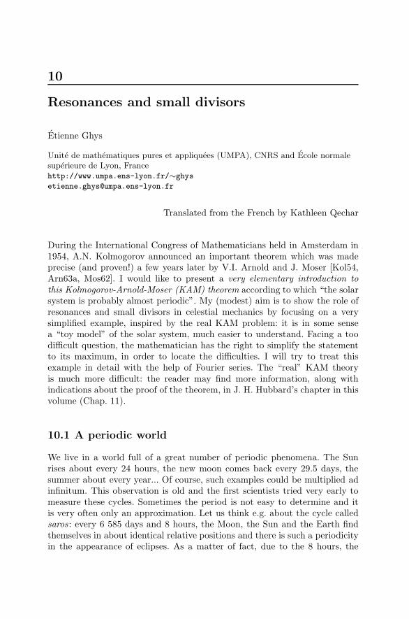
Mathematicians have always been fascinated by cycles and one did nothave to wait for Fourier to decompose a cyclic phenomenon into a sum ofelementary cyclic phenomena. What is more elementary than a point whichrotates on a circle with a constant angular velocity? It is of course the modelthe first observers of the Sun (which rotates “evidently” around the Earth)were thinking about. The situation is a little more complicated in the caseof planets, as the paths they follow in the sky seem sometimes complex (seeFig. 10.1).

Fig. 10.1. Mercury’s orbit seen from the Earth (“Terre”). (From Flammarion’sAstronomie Populaire.)

10 Resonances and small divisors 189

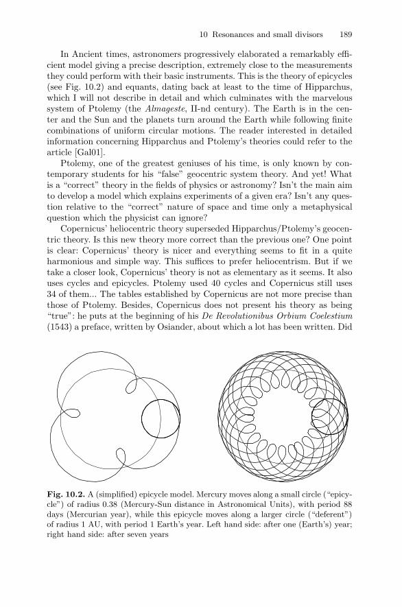
In Ancient times, astronomers progressively elaborated a remarkably effi-cient model giving a precise description, extremely close to the measurementsthey could perform with their basic instruments. This is the theory of epicycles(see Fig. 10.2) and equants, dating back at least to the time of Hipparchus,which I will not describe in detail and which culminates with the marveloussystem of Ptolemy (the Almageste, II-nd century). The Earth is in the cen-ter and the Sun and the planets turn around the Earth while following finitecombinations of uniform circular motions. The reader interested in detailedinformation concerning Hipparchus and Ptolemy’s theories could refer to thearticle [Gal01].

Ptolemy, one of the greatest geniuses of his time, is only known by con-temporary students for his “false” geocentric system theory. And yet! Whatis a “correct” theory in the fields of physics or astronomy? Isn’t the main aimto develop a model which explains experiments of a given era? Isn’t any ques-tion relative to the “correct” nature of space and time only a metaphysicalquestion which the physicist can ignore?

Copernicus’ heliocentric theory superseded Hipparchus/Ptolemy’s geocen-tric theory. Is this new theory more correct than the previous one? One pointis clear: Copernicus’ theory is nicer and everything seems to fit in a quiteharmonious and simple way. This suffices to prefer heliocentrism. But if wetake a closer look, Copernicus’ theory is not as elementary as it seems. It alsouses cycles and epicycles. Ptolemy used 40 cycles and Copernicus still uses34 of them... The tables established by Copernicus are not more precise thanthose of Ptolemy. Besides, Copernicus does not present his theory as being“true”: he puts at the beginning of his De Revolutionibus Orbium Coelestium(1543) a preface, written by Osiander, about which a lot has been written. Did

Fig. 10.2. A (simplified) epicycle model. Mercury moves along a small circle (“epicy-cle”) of radius 0.38 (Mercury-Sun distance in Astronomical Units), with period 88days (Mercurian year), while this epicycle moves along a larger circle (“deferent”)of radius 1 AU, with period 1 Earth’s year. Left hand side: after one (Earth’s) year;right hand side: after seven years

190 Etienne Ghys

Osiander want to protect Copernicus from the pope’s ire? Or on the contrarydoes this preface reflect Copernicus’ opinion? Here is an extract from thispreface (see [Cop92]):

... it is the duty of an astronomer to compose the history of the celestial

motions through careful and expert study. Then he must conceive and devise

the causes of these motions or hypotheses about them. Since he cannot in

any way attain to the true causes, he will adopt whatever suppositions

enable the motions to be computed correctly [...] these hypotheses need

not be true nor even probable. On the contrary, if they provide a calculus

consistent with the observations, that alone is enough.

Let us return to our cycles. If a phenomenon is periodic with period T , all mul-tiples of T can also be considered as a period. Consequently, if two phenomenahave respectively a period T1 and T2, the combination of these phenomenawill be periodic as soon as a multiple of T1 coincides with a multiple of T2,in other words as soon as the ratio T1/T2 is a rational number. Since we aretalking about astronomy and these periods can only be known approximately,we can consider that these ratios are always (almost) rational. The combina-tions of the cycles that we observe in our universe define therefore a globallyperiodic phenomenon. A reader could quite rightly notice that this type of ar-gument may easily lead to gigantic periods and that the physical meaning ofa period of e.g. one hundred billion years would be questionable. This readermay be reassured: this question is somehow at the heart of this article andour (pre-pythagorician) “physical hypothesis” that all numbers are rationalwill be discussed and modified all along this article. Let us therefore start byimagining that all physical functions are periodic...

The idea of combining circles to approach a periodic function may not bedue to Hipparchus and Ptolemy but in respect for these geniuses, I would liketo attribute them the joint property of the following theorem:

Theorem. [Hipparchus-Ptolemy-Fourier] Let f : R → C denote a contin-uous periodic curve of period T with values in the complex plane. Thenf may be arbitrarily closely approximated by a finite combination of uni-form circular motions. In other words, for any ε > 0, there exists a func-tion of the form fε(t) =

∑Nn=−N an exp(2iπnt/T ) (with an ∈ C) such that

|f(t)− fε(t)| < ε for all t.

Clearly, Hipparchus and Ptolemy did not prove this theorem in the modernsense of the term but neither did Fourier1. For a “modern proof”, the readercan refer to e.g. [Kor89].

1 A “theorem” attributed to V.I. Arnold asserts that on one hand no theorem isdue to the mathematician which it is named after and on the other hand thatthis theorem applies to itself.


1. An adelic fantasy.

I would like to allow myself a mathematician’s fantasy which is totally useless forthe rest of this article and which the reader may skip. The time of contemporaryscience is modeled by the set R of real numbers (even if it has been subject toseveral avatars with the relativity theories). This set does not suggest the ideaof successive cycles which we have just mentioned: it flows inexorably from thepast to the future. Let us try to formalize time the same way astronomers suchas Ptolemy used to think about it, formed by cycles “piled up one on top of theother”, in which recurrences are omnipresent.

For any integer n > 0, the quotient R/nZ formed by real numbers modulo

n represents the “cyclic time of period n”. If m and n are two integers such

that m divides n, there is an obvious projection πm,n from the cycle R/nZ to

the cycle R/mZ: if we know a real number modulo n, we know it in particular

modulo m. Let us define the cyclic time T as follows: an element t in T is a

map which associates to any integer n an element tn of R/nZ in a way which is

compatible with these natural projections, i.e. in such a way that if m divides n,

then we have πn,m(tn) = tm. In other words, an element of T is a way to place

oneself in all cycles while respecting the evident compatibilities. Obviously, the

“cyclic time” T contains the “ordinary time” R: to a given real number t, we can

associate for every n the point t modulo n in R/nZ and these various points are

compatible with each other. But T is much bigger than R (exercise). We can equip

T with a topological structure which turns it into a compact topological group

(exercise). Time as a compact set... a mathematician’s (or oriental philosopher’s?)

dream which illustrates the idea of recurrence. The usual group of real numbers

R is contained as a dense subgroup of T (exercise). Can one consider T as a

reasonable psychological model for the time we are actually living in? Is this a

futile mathematician’s exercise? Maybe not. The group T we have just introduced

is the “adelic torus”, the study of which is essential in contemporary number

theory.

10.2 Kepler, Newton. . .

I will not describe in detail the marvelous astronomical works of Kepler whichare often summarized as Kepler’s three laws. The first one states that a planetorbits as a conic with the Sun at one focus. The second (law of areas) describesthe speed at which this conic is traversed. The third law expresses the period(in the case of an elliptic motion) in terms of the major axis of the ellipse. Allof this is far too well-known and can easily be found in many books dealingwith rational mechanics. At this point, I would like to insist on two less well-known aspects of Kepler’s work.

192 Etienne Ghys

Kepler is often “blamed” to have only offered a descriptive and nonex-planatory model: what causes the motion of the planets? Newton’s law f = mγand the gravitational attraction in 1/r2 are wonders but do they explain morethan Kepler why objects attract each other? This is similar to the compari-son Ptolemy/Copernicus: Newton’s laws prevail over those of Kepler by theiraesthetic aspect and because they allowed a revolution in physics (and inmathematics). However, they do not explain the cause of the phenomenon(and of course, I could make the same kind of comments on the explanatorycharacter of general relativity).Kepler’s zeroth law : if the orbit of a planet is bounded, it is periodic, i.e. itis a closed curve.

If one thinks about this, it is incredible.Nowadays, one can show the following result (Bertrand’s theorem, al-

ready known to Newton?). Let us suppose that a material point movesin the plane while being attracted towards the origin of the plane (theSun) by a force whose modulus F (r) only depends on the distance r tothe origin. Let us suppose that all the orbits which are bounded are infact closed curves. Then, the force F (r) can only be the Newtonian attrac-tion F (r) = k/r2 or the elastic attraction F (r) = Kr (not very reason-able in astronomy!). Why did “mother Nature” “choose” THE law that en-sures the periodicity of motion? This is a mystery physics will not explainsoon!

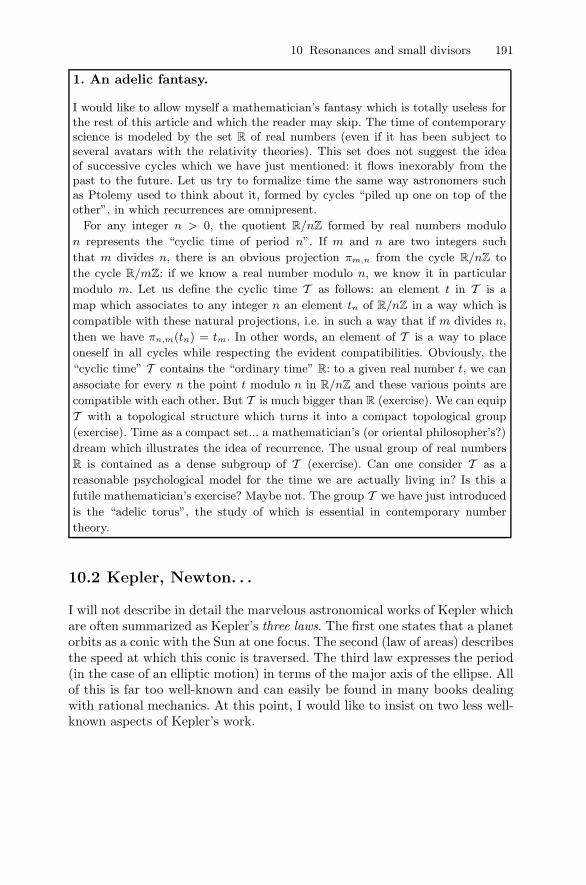
How is the motion of a planet if the force of attraction towards the centralpoint is another function F (r)? This is a classical question of mechanics andNewton himself studied a great number of cases in his Principia (1687). Abounded orbit consists of arcs which join the successive apogees and perigees(see Fig. 10.3). These arcs are obtained from one of them using a symmetryand rotations, the angle of which depends on the considered orbit. Somehow,we can consider that the motion is the result of two periodic phenomena:one relates to the periodic variation of the distance to the Sun and the other

Fig. 10.3. An almost periodic orbit (between the apoapsis and periapsis circles).LHS: an apoapsis and the subsequent periapsis; RHS: after several turns


relates to the periodic variation of the direction of the straight line joiningthe Sun to the planet. The orbit is periodic if the two periods have a rationalratio and it is almost periodic otherwise. Only the forces in r and 1/r2 aresuch that this ratio is always rational and it happens that it is then equalto 1, so that in these two cases the orbits close themselves in fact after onecomplete turn. The law 1/r2 is a resonance of nature since it corresponds tothe equality of the radial and angular frequencies.

Kepler must have been filled with wonder when he realized that the orbitof Mars is periodic. This statement is not very obvious when we observe itfrom the Earth and that does not follow in any way from the epicycle modelsof Hipparchus-Ptolemy-Copernicus.

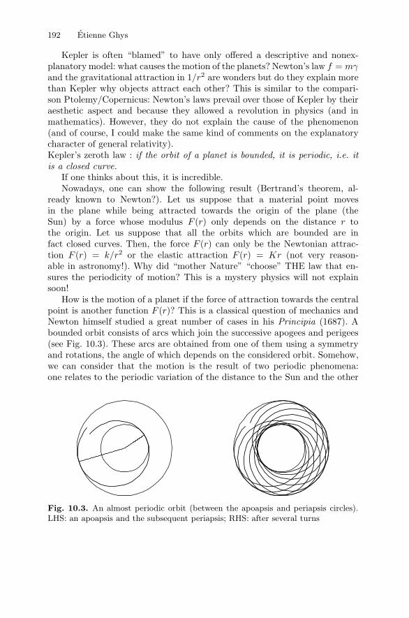
I should also mention Kepler’s “fourth” law which is rarely cited becauseit is false, but which Kepler considered as his main discovery. This law wasmeant to explain the numerical values of the major axes of the orbits of thesix planets (which were known at that time). The construction is marvellous,almost philosophical: it is a question of successively encasing the five regular(Platonic) polyhedrons in inscribed and circumscribed spheres (see the beau-tiful Fig. 10.4 extracted from Harmonices Mundi (1619)): the radiuses of thespheres give the radiuses of the orbits (up to similarity of course). Should wemake fun of this? Of course not, because it seems that the obtained result isvery close to reality and especially because it is an attempt of geometrizationof space and motion. Other attempts were very successful later in history.In [Ste69], Sternberg encourages those who make fun of Kepler to also makefun of contemporary theoretical physicists who relate the elementary parti-cles to linear representations of simple Lie groups. The search for groups ofsymmetries is at the heart of science no matter what the subject is: the icosa-hedron group, gauge groups, or approximate symmetries in an almost periodicmotion, or in a quasicrystal.

Fig. 10.4. Harmonices Mundi

194 Etienne Ghys

10.3 An almost periodic world

Thus, the world we inherited from Hipparchus, Ptolemy, Kepler and Newtonis a periodic world. More precisely, each planet is periodic but the solar systemis “almost periodic” in its totality since there is of course no reason that theratios of the periods of the different planets are rational numbers.

Irrational numbers do exist. The sum of two periodic functions whoseperiods have an irrational ratio is not periodic. But it almost is... The formal-ization of this idea is recent. Let us begin with two “reasonable” definitions:

Definition. Let f denote a continuous function from R to C and ε > 0 a(small) positive real number. A real number T is an ε-period if for every t inR, one has : |f(t+ T )− f(t)| < ε.

Definition. Let f denote a continuous function from R to C. We say that fis almost periodic if for every ε > 0, there exists a number M > 0 such thatevery interval in R with length greater than M contains at least one ε-period.

The theory of almost periodic functions is rich. The interested reader may readthe book [Ste69], in particular for its link with the history of the celestialmechanics. Here are two theorems. The first one is rather an exercise whichis left to the reader:

Theorem. Let a1, . . . , ak be complex numbers and ω1, . . . , ωk real numbers.The function f from R to C defined by f(t) =

∑kn=1 an exp(iωnt) is almost

periodic.

The second theorem is much more complicated. Formally, it is due to Bohrbut for the same subjective reasons as those exposed earlier, I also attributeit to Hipparchus and Ptolemy.

Theorem. [Hipparchus-Ptolemy-Bohr] Every almost periodic function maybe arbitrarily closely approximated by functions of the preceding type.

Now that these definitions and theorems are presented, I can start to makethe content of this article more precise. Is the universe in which we live almostperiodic?

10.4 Lagrange and Laplace: the almost periodic world

The proof of Kepler’s laws using from those of Newton supposes a “simplified”solar system in which a single planet is attracted by a fixed center. One learnsin elementary courses of mechanics that the problem is not much more diffi-cult in the case of two masses which attract each other mutually: each one ofthem describes a conic. But of course, there is not only one planet in the solarsystem. Even disregarding many “small” objects, we can consider that nine2

2 This paper was written before Pluto was “expelled” from the official list of planets!


2. A remark about the recent history of Physics.

The turbulence of fluids is a quite complex phenomenon which has been puz-

zling physicists for a long time, at least starting from Leonardo da Vinci, and

whose practical applications are more than obvious in aeronautics. How can we

understand these eddies of all sizes in turbulent fluids, and the flow of energy from

larger eddies towards smaller ones, up to the dissipative scales (Kolmogorov’s the-

ory [Kol41])? It is astonishing to note that physicists as eminent and imaginative

as Landau and Lifschitz presented for a long time turbulence as an almost periodic

phenomenon, of which the number of frequencies depends on the Reynolds num-

ber (related in particular to the viscosity of the fluid). It is only with the second

edition (1971) of their famous treatise on fluid mechanics that they became aware

that the almost periodic functions are too “well behaved” to represent this phe-

nomenon and that it is necessary to call upon much more “chaotic” functions: it

is the beginning of the theory of strange attractors, a beautiful example of collab-

oration between mathematicians and physicists. Old habits are difficult to loose:

the epicycles are still present in our scientific subconscious and it is difficult to get

rid of them. Should we forget the epicycles and almost periodic functions in the

description of our solar system? Are the conservative systems, such as the solar sys-

tem, also subject to some kind of chaos (and in which sense?), as in the case of the

dissipative systems (turbulence)? Somehow, the theorem of Kolmogorov-Arnold-

Moser is reassuring: it asserts that under good conditions (explained further on),

the almost periodic functions are sufficient to describe the motion of planets.

planets orbit the Sun and attract each other mutually. This N -body problemis mathematically far more complicated and in a sense which I cannot describeprecisely here, it has been known since the beginning of the twentieth centurythat it is impossible to “integrate” it.

For lack of finding “workable” exact solutions for the motion, we are re-duced to finding approximate solutions. Lagrange and Laplace are prominentamong those who developed best the theory of perturbations. Of course, asa first approximation, the dominant forces in the solar system are the forcesof attraction towards the Sun because the mass of the Sun is much biggerthan those of the other planets (in a ratio of approximately 103). We can thusthink that the planets will more or less follow the (periodic) elliptical Keple-rian orbits and that those ellipses will change slowly because of the perturbinginfluence of other planets. How important are these small perturbations? Arethey likely to significantly modify the harmony of the Keplerian system? Theseare difficult questions. We could fear the worst: perhaps a perturbing force ofthe order of 1/1000 times the principal force could significantly modify theradius of an orbit after a time of about a thousand times the characteristictime of the problem (the year). In other words, we could fear that within athousand years, the radius of the terrestrial orbit may be divided (or mul-tiplied) by two. This would have important consequences on the history of

196 Etienne Ghys

our civilization! Since we did not notice any catastrophe of this kind in ourpast, what is the phenomenon that explains why the perturbations perturbless than what we could fear?

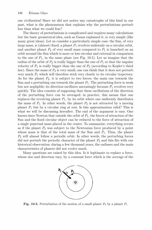
The theory of perturbations is complicated and requires many calculationsbut the basic geometrical idea, such as Gauss explained it, is very simple (likemany great ideas). Let us consider a particularly simple case: the Sun, of verylarge mass, is (almost) fixed; a planet P1 revolves uniformly on a circular orbit,and another planet P2 of very small mass compared to P1 is launched on anorbit around the Sun which is more or less circular and external in comparisonto the one of P1, in the same plane (see Fig. 10.5). Let us imagine that theradius of the orbit of P2 is really bigger than the one of P1 so that the angularvelocity of P1 is really bigger than the one of P2 (according to Kepler’s thirdlaw). Since the mass of P2 is very small, one can think that it does not perturbvery much P1 which will therefore stick very closely to its circular trajectory.As for the planet P2, it is subject to two forces: the main one towards theSun and a perturbing one towards the planet P1. The perturbing force is weakbut not negligible; its direction oscillates unceasingly because P1 revolves veryquickly. The idea consists of supposing that these oscillations of the directionof the perturbing force can be averaged: in practice, this means that onereplaces the revolving planet P1, by its orbit where one uniformly distributesthe mass of P1. In other words, the planet P2 is not attracted by a movingplanet P1 but by a circular ring at rest. Is this approximation valid? This iswhat we will be discussing hereafter. The end of the argument is easy. Oneknows since Newton that outside the orbit of P1, the forces of attraction of theSun and the fixed circular object can be reduced to the force of attraction ofa single punctual mass placed in the center. To summarize, everything occursas if the planet P2 was subject to the Newtonian force produced by a pointwhose mass is that of the total mass of the Sun and P1. Thus, the planetP2 will almost follow a periodic orbit. In other words, the perturbing forcesdid not perturb the periodic character of the planet P2 and this fits with ourhistorical observation: during a few thousand years, the radiuses and the maincharacteristics of planets did not evolve much.

Many questions are raised by this idea. Is it legitimate to replace a force,whose size and direction vary, by a constant force which is the average of the

Fig. 10.5. Perturbation of the motion of a small planet P2 by a planet P1


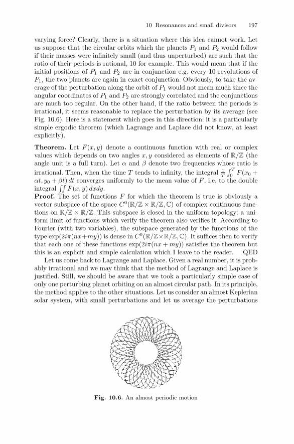
varying force? Clearly, there is a situation where this idea cannot work. Letus suppose that the circular orbits which the planets P1 and P2 would followif their masses were infinitely small (and thus unperturbed) are such that theratio of their periods is rational, 10 for example. This would mean that if theinitial positions of P1 and P2 are in conjunction e.g. every 10 revolutions ofP1, the two planets are again in exact conjunction. Obviously, to take the av-erage of the perturbation along the orbit of P1 would not mean much since theangular coordinates of P1 and P2 are strongly correlated and the conjunctionsare much too regular. On the other hand, if the ratio between the periods isirrational, it seems reasonable to replace the perturbation by its average (seeFig. 10.6). Here is a statement which goes in this direction: it is a particularlysimple ergodic theorem (which Lagrange and Laplace did not know, at leastexplicitly).

Theorem. Let F (x, y) denote a continuous function with real or complexvalues which depends on two angles x, y considered as elements of R/Z (theangle unit is a full turn). Let α and β denote two frequencies whose ratio isirrational. Then, when the time T tends to infinity, the integral 1

T

∫ T0 F (x0 +

αt, y0 + βt) dt converges uniformly to the mean value of F , i.e. to the doubleintegral

∫∫F (x, y) dxdy.

Proof. The set of functions F for which the theorem is true is obviously avector subspace of the space C0(R/Z× R/Z,C) of complex continuous func-tions on R/Z× R/Z. This subspace is closed in the uniform topology: a uni-form limit of functions which verify the theorem also verifies it. According toFourier (with two variables), the subspace generated by the functions of thetype exp(2iπ(nx+my)) is dense in C0(R/Z×R/Z,C). It suffices then to verifythat each one of these functions exp(2iπ(nx+my)) satisfies the theorem butthis is an explicit and simple calculation which I leave to the reader. QED

Let us come back to Lagrange and Laplace. Given a real number, it is prob-ably irrational and we may think that the method of Lagrange and Laplace isjustified. Still, we should be aware that we took a particularly simple case ofonly one perturbing planet orbiting on an almost circular path. In its principle,the method applies to the other situations. Let us consider an almost Kepleriansolar system, with small perturbations and let us average the perturbations

Fig. 10.6. An almost periodic motion

198 Etienne Ghys

on their configuration spaces. We hope that there are no resonances, i.e. norational linear relations between the periods which appear. This leads to thestability theorem of Laplace which asserts that in the averaged system, themajor axes of the orbits remain constant in time, ensuring a certain stabilityto the system. Finally, this “justifies” the fact that the effects of perturbationsare smaller than the ones we could fear a priori.

What kind of mathematical credit can we give to this type of “proof”? If weseek “true stability theorems” which are valid for infinitely long times, we willfind nothing in Laplace’s works which resembles a proof, and the assertionswhich we sometimes meet according to which “Laplace showed the stabilityof the solar system” are largely exaggerated. On the other hand, if we seekmathematical statements which are valid for long but finite times, we can hopeto transform these methods into theorems, at least in certain particular cases.No matter what, this kind of method lets us think that if the perturbationsare of the order of ε (10−3 in our system), these perturbations have no globaleffect at a time 1/ε as we might expect a priori but rather after a time 1/ε2

(“the next term in an asymptotic expansion”). We should have a quiet life forabout 106 years, which is more reasonable than 103. The reader who would liketo know more about these perturbation methods may consult some treatiseson celestial mechanics if he is brave enough or [Arn89, Arn83, AA68] for aconceptual presentation.

Thus, we inherit from Lagrange and Laplace an almost periodic world,at least for a million years! But they also leave us many questions: what isthe role of these resonances between the periods of the planets which putin danger the averaging arguments? Is the stability of the motion perpet-ual or does it get destroyed after a million years? How can we make this“stability theorem of Laplace” rigorous? It took almost two centuries andthe works of mathematicians as powerful as Poincare, Siegel, Kolmogorov,Arnold and Moser to get to partial answers which themselves raised otherquestions.

10.5 Poincare and chaos

At the end of the nineteenth century, Poincare invented rigorous geometricmethods in order to approach a global understanding of the N -body prob-lem. As a matter of fact, he focused on the restricted three-body problem: twopunctual bodies orbit in a Keplerian way in a plane, around their center ofmass, and a third punctual body, with infinitely small mass, is subject tothe attraction of the two other masses. Here are some questions studied byPoincare in his famous article Sur le probleme des trois corps et les equationsde la dynamique (1890) [On the three-body problem and the equations of dy-namics]. Is the trajectory of the small mass confined in a bounded domainof the plane if its total energy is sufficiently small? For an initial “generic”condition, is there a risk of collision between the bodies? Is the dynamical


behavior of the small body almost periodic? Unfortunately I will not de-scribe this historical article of Poincare. I will only point out that Poincareproves the existence of a great number of periodic orbits and that he at-tempts to understand the dynamics in the vicinity of these periodic orbits.At that point, he makes an error and sins by optimism in a proof (he is usedto doing so): his great memoir awarded by king Oscar of Sweden is false. Inhaste, he has to correct it and this correction will prove to be of consider-able scientific richness: Poincare creates on this occasion the theory of chaos.He highlights trajectories whose behaviors are very far from being almostperiodic:

“Let us try to represent the figure formed by these two curves andtheir infinite number of intersections each one of which correspondsto a doubly asymptotic solution, these intersections form a kind ofweb, of fabric, of network with infinitely tight meshes; each one ofthese curves should never intersect itself, but it must fold up it-self in a very complex way to come to cut infinitely often all themeshes of the network. One will be struck by the complexity of thisfigure, which I do not even attempt to draw. There isn’t anythingmore proper to give us an idea of the complication of the three-bodyproblem and, in general, of all the problems of dynamics where thereis no uniform integral and where the Bohlin series are divergent.”(Poincare [Poi90])

The history of this error and the way in which Poincare transforms it intosuccess is fascinating. I recommend the book [Bar97] which is entirely devotedto this question, and the article [Yoc06].

Thus, even if the initial conditions which lead to these examples of chaotictrajectories are not very close to the physical conditions of our solar system,we know thanks to Poincare that the orbits of the celestial bodies are notnecessarily almost periodic. Will we find such orbits in our solar system? Inany case, it is necessary for us to be more modest in our search of stability.Previously, we sought to know whether the orbits of planets are almost pe-riodic and we are now much less ambitious since the question becomes thefollowing one. If we launch the planets of a solar system on almost circularorbits around a Sun with very great mass, will the planets remain foreverconfined in a bounded domain of space? Might it be possible that a planet beejected from the system for example?

10.6 A “toy model” of the theory of perturbations

We are going to build up a very simple (and even naive) model. On thecylinder R/Z × R, let us consider the transformation f which associates tothe point (x, y) the point (x + α, y) where α is an irrational angle. We are

200 Etienne Ghys

going to iterate this transformation and study its dynamics. This is a firstsimplification: instead of studying dynamics in continuous time (in R), we aregoing to use a discrete time (in Z). After n iterations, the point (x, y) is sent tothe point (x+nα, y) so that the orbits of f spread on the circles y = const. Wecan thus think about f as the dynamics of an almost periodic system. Now,let us try to perturb the motion by imposing to our point of R/Z×R a “push”towards the top or the bottom which only depends on the first coordinate.In other words, we are now studying a transformation g which associates tothe point (x, y) the point (x + α, y + u(x)) where u is a certain very regularfunction defined on R/Z (i.e. a periodic function of period 1) which we canthink of as being a small perturbation. What is the new dynamics? The n-thiteration of g maps the point (x, y) to the point (x+ nα, y + u(x) + u(x+ α)+ · · ·+ u(x+ nα)).

Lagrange’s averaging principle suggests to replace the impulse u by itsaverage on the circle. Of course, if this average is different from 0, we caneasily understand that the successive iterations of g will have a tendency tomake the second coordinate tend to infinity so that the perturbed system isnot stable. Thus, let us study the situation when the average of u on thecircle is equal to 0: on average the second coordinate is not modified. Canwe deduce that g is stable, in the sense that its orbits stay bounded? This isthe simplified problem we are going to study. In symbols, the question is thefollowing:

Let u denote a periodic function of period 1, which is infinitely differen-tiable, and whose integral on a period is equal to 0. Let α denote an irra-tional number and x a real number. Are the (absolute values of the) sumsu(x) + u(x + α) + · · · + u(x + nα) bounded when the “time” n tends toinfinity?

Let us begin with a lemma which is a special case of a lemma of Gottschalkand Hedlund:

Lemma. Let us fix x0 in R/Z. The absolute values of the sums u(x0)+u(x0 +α) + · · · + u(x0 + nα) are bounded if and only if there exists a continuousfunction v on R/Z such that for all x one has u(x) = v(x+ α)− v(x).

Proof. If u(x) is of the form v(x+ α)− v(x), the above sum “telescopes” to:u(x0) + u(x0 + α) + · · · + u(x0 + nα) = v(x0 + (n + 1)α) − v(x0). Thus itsmodulus is bounded by twice the maximum of |v| (which is finite because vis periodic and continuous).

Conversely, let us assume that |u(x0) + u(x0 + α) + · · · + u(x0 + nα)| isbounded by M > 0. This means that the orbit of the point (x0, 0) in thecylinder R/Z×R stays confined in the compact cylinder R/Z× [−M,M ]. LetK denote the closure of this orbit. This is a compact set which is invariantunder the transformation g. Among all the non-empty compact sets containedin K and invariant under g, let us choose one which is minimal for inclusion


(use the property that the intersection of a family of non-empty compact sets,which is totally ordered for inclusion, is not empty) and let us denote it byM. I claim that M is the graph of a continuous function v from R/Z to R.

To justify this assertion, I first observe that the projection of M on thefirst coordinate is a non-empty compact set in the circle, which is invariantunder the rotation with irrational angle α. All the orbits of such a rotation aredense in the circle. Consequently, the projection of M on the first coordinateis necessarily the full circle R/Z.

Now, let me prove that for each x in R/Z, the “vertical” line {x} × R

only meets the minimal set M in one point. In order to prove this state-ment, I consider the vertical translations τt(x, y) = (x, y + t). Obviously,these translations commute with g so that the image by τt of an invariantset under g is also an invariant set under g. Consequently, τt(M) is in-variant under g and so are the intersections τt(M) ∩ M. We have chosenM as a minimal non-empty compact invariant set. It follows that for all t,the intersection τt(M)

⋂M is either empty or equal to M. But if τt(M)

would coincide with M for a t different from 0, then M would be equalto τkt(M) for every integer k and would not be bounded (let k tend to in-finity). Therefore τt(M) and M are disjoint when t is different from 0 andthis means that M meets each vertical {x} × R at a unique point (x, v(x)).Thus, M is the graph of a function v of R/Z to R. As this graph is com-pact, the function v is continuous (a traditional exercise). The assertion isproven.

We still have to express analytically that the graph of the function v isinvariant under the transformation g. The image of (x, v(x)) is (x+α, v(x) +u(x)) and has to be equal to (x+α, v(x+α)). We obtain as expected u(x) =v(x+ α)− v(x) and the lemma is proven. QED

Before continuing, let me restate the lemma in a geometric way. As soon asan orbit of the transformation g is bounded, it remains confined in an invariantcircle which is the graph of a continuous function. All the other orbits are thenbounded. In other words, in this case, the family of circles y = const which isinvariant under the non-perturbed transformation f is replaced by the familyof perturbed circles y − v(x) = const which is invariant under the perturbedtransformation g.

This leads to a question of harmonic analysis. Given an infinitely differ-entiable function u whose integral on the circle is equal to 0, and given alsoan irrational number α, does there exist a continuous function v on the circlesuch that u(x) = v(x+ α)− v(x) identically?

The Fourier series are particularly well adapted to study this problem.As the function u is infinitely differentiable, it can be expanded as a Fourierseries:

u(x) =+∞∑

−∞un exp(2iπnx).

202 Etienne Ghys

Let us also seek the function v through its Fourier series expansion (we willdiscuss the convergence of this series afterwards):

v(x) =+∞∑

−∞vn exp(2iπnx).

(I use the complex notation for convenience: as the function v is real, thecomplex numbers vn and v−n are conjugate). Then we have:

v(x+ α)− v(x) =+∞∑

−∞(exp(2iπnα)− 1)vn exp(2iπnx).

Identifying the Fourier coefficients of u(x) and of v(x + α) − v(x), we thusobtain:

vn =un

(exp(2iπnα)− 1)·

The assumption according to which α is irrational means that (exp(2iπnα)−1) is different from 0 for n different from 0. Therefore the vn’s are well definedfor n different from 0. For n = 0, our hypothesis on the average of u meansprecisely that u0 = 0 so that we can choose any value for v0 (which of coursecorresponds to the fact that if v is a solution to our problem, v+ const is alsoa solution).

To summarize, Lagrange’s principle seems to work. We have certainlyfound a function v which is a solution to our functional equation, or at leastits Fourier series expansion. But does this series converge and does it definea continuous function as we expect? This is our new problem.

3. How can we “see” on a Fourier series that it definesa regular function?

Let us consider a periodic function h of period 1 and let us expand it as a Fourierseries:

h(x) =

+∞∑

−∞hn exp(2iπnx).

How can we “see” on the sequence of coefficients hn that the function h is infinitelydifferentiable for example? If the function h is supposed to be continuous and notmore, is the sequence hn subject to some constraints? These are delicate questions(which Fourier did not seem to have considered) about which we nowadays knowa lot. In this interlude, I will simply give some very elementary observations whichwill suffice for my discussion. The n-th coefficient hn is given by Fourier’s formula:

hn =

∫

R/Z

h(x) exp(−2iπnx) dx.

If h is continuous, then the sequence hn must be bounded. Caution: the converse

is very far from being valid and my bound is rather crude. One can prove e.g. that

the sequence hn tends in fact to 0 and that the series (nh1 +(n−1)h2 +· · ·+hn)/n

is convergent.


If h is continuously differentiable, we can calculate the Fourier coefficients h′n

of its derivative by the well-known formula h′n = 2iπnhn. The continuity of the

derivative and the previous observation show that there is an estimate for thedecay at infinity of hn of the form |hn| < Cst/|n|. If h is infinitely differentiable,we can repeat this argument for all derivatives. Thus, the Fourier coefficients ofan infinitely differentiable function have a rapid decay. This means that for everyinteger k, there exists a constant Ck > 0 such that |hn| < Ck |n|−k.Conversely, let us consider a rapidly decreasing sequence hn and let us form itsassociated Fourier series. It is easy to prove that this series is indeed convergentand defines an infinitely differentiable function.

These simple remarks will suffice but it is a pity to have to leave such a topic

without having really gotten into it. The book [Kor89] is magnificent (but requires

more mathematical technique).

4. Numbers which are more or less irrationals?

Every irrational number may be arbitrarily approximated by rational numbers.Let us try to make this assertion quantitative. Let α denote an irrational realnumber. Let us fix a (small) real number ε > 0 and let us seek a rational numberp/q (where q > 0) such that |α − p/q| < ε. Such a p/q always exists but if ε isvery small, a rational p/q which verifies this inequality has necessarily a very largenumerator and denominator. What is the minimal value of q as a function of ε?At what speed does this function tend to infinity when ε tends to 0? All dependson the irrational number being considered. In this interlude, we present the basicsof the theory of diophantine approximation, which is important in our problem.Some numbers are exceptionally well approximated by rational numbers. The mostfamous example is the number defined by Liouville:

λ =

+∞∑

n=1

10−n! = 0.1100010000000000000000010000000000000000000000000 . . .

If we truncate the series at order n, we find a rational number whose denomina-

tor is 10n! and which approximates λ with a difference smaller than 2.10−(n+1)!,

which is extraordinarily small in comparison to the inverse of the denomina-

tor 10n!. For any physicist, this number is rational since it is different from

0.110001000000000000000001 by less than 10−120 which is a lot smaller than

any physically observable number. Nevertheless, not only does the mathemati-

cian know that λ is irrational (its decimal expansion is not periodic) but also that

Liouville has proven that λ is in fact a transcendental number. If the reader is

not impressed by the approximation speed of λ, he may replace the factorials n!

by double factorials n!! or even by any increasing function from N to N, which

may even be non-recursive. Thus, given any function ε(q) from positive integers

to positive numbers, tending to zero when q tends to infinity, we can always find

irrational numbers α which are approximated by rationals “better than ε(q)”, i.e.

for which there exists infinitely many rationals p/q such that |α − p/q| < ε(q).

Some irrational numbers resist to the approximation as much as they possibly

204 Etienne Ghys

can. A lemma of Dirichlet shows that every irrational number may be approxi-mated by rationals “up to 1/q2”:

Lemma. For any irrational number α, there exists infinitely many rationals p/q(q > 0) such that |α − p/q| < 1/q2.Proof. Let us project the first N + 1 multiples 0, α, . . . , Nα in the circle R/Z.At least two of these projections are at a distance smaller than 1/(N + 1) in thecircle. This means that we can find 0 ≤ k1 < k2 ≤ N such that (k2 − k1)α is at adistance less than 1/(N + 1) of an integer p. Writing q = k2 − k1 ≤ N , we obtain|qα − p| < 1/(N + 1) < 1/q. We observe that |qα − p| < 1/(N + 1) implies that qtends to infinity when N tends to infinity. QED

Definition. An irrational number α is diophantine if there exists a constant

C > 0 and an exponent r ≥ 2 such that for any rational p/q (q > 0) one has

|α − p/q| > C/qr.

5. A diophantine number: the golden mean

The most famous example of a number which is badly approximated by the ra-tionals is the golden mean φ = (1 +

√5)/2.

Theorem. There exists a constant C > 0 such that for every rational p/q, wehave |φ − p/q| > C/q2.

In fact, we could even prove that we may take C = 1/√

5 and that φ is theirrational number which has the worst approximation by rationals (see [Niv56] fora precise statement and for further details on these questions of approximationby rationals).

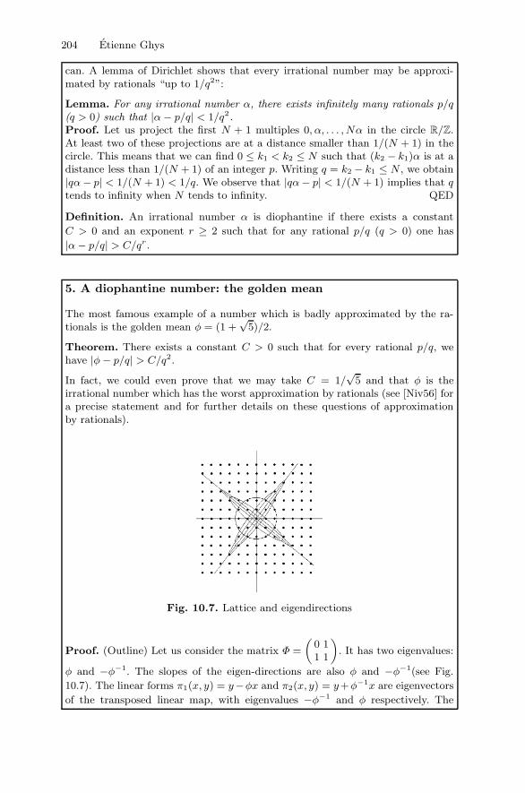
Fig. 10.7. Lattice and eigendirections

Proof. (Outline) Let us consider the matrix Φ =

(0 11 1

). It has two eigenvalues:

φ and −φ−1. The slopes of the eigen-directions are also φ and −φ−1(see Fig.

10.7). The linear forms π1(x, y) = y−φx and π2(x, y) = y +φ−1x are eigenvectors

of the transposed linear map, with eigenvalues −φ−1 and φ respectively. The


matrix Φ acts linearly in the plane R2 and preserves the two eigen-lines as well

as the lattice of integral points since its coefficients and those of its inverse areintegers. Note that Φ dilates the first eigen-line (φ > 1) and contracts the otherone. We are seeking to measure the degree of approximation of φ by rationals. Inother words, we are looking for points on the line of slope φ whose coordinatesare “as integral as possible”. Let us consider a disk D big enough in the planewhose center is the origin. In this disk, there is only a finite number of pointswith integral coordinates, so that there exists a constant C1 > 0 such that for allintegral points in D different from (0, 0), we have: |π1(q, p)π2(q, p)| > C1. Let usstudy the effect of the action of the matrix Φn. The disk D is transformed in theinterior Dn of an ellipse, laid down along the line of slope φ, and the estimate|π1(q, p)π2(q, p)| > C1 for the integral points (q, p) different from 0 and located inD implies the same inequality for allintegral points of Dn different from 0. This is clear because the product |π1π2| isinvariant under the action of Φ. Thus the inequality |π1(q, p)π2(q, p)| > C1 is validfor all integral points in all the Dn’s. When n varies in Z, these Dn’s cover a whole“hyperbolic” neighborhood of the eigen-lines, of the form |π1(x, y)π2(x, y)| < C2.

To summarize, we have proven that there exists a constant C3 = min(C1, C2)

such that for any integral point (q, p) of the plane (different from (0, 0)), we have

|π1(q, p)π2(q, p)| > C3. Now, let us distinguish two sets of rationals p/q according

to whether |φ − p/q| is greater than or less than a fixed small enough quantity

C4 > 0. On the first set, the inequality |φ − p/q| ≥ C4 implies in particular that

|φ − p/q| ≥ C4/q2. On the second set, the inequality |φ − p/q| < C4 implies an

inequality of the form |π2(q, p)| > C5|q| (in fact C5 = φ + φ−1 − C4 =√

5 − C4 is

appropriate) so that we have |π1(q, p)| > C3C−15 /|q| and so |φ−p/q| > C3C

−15 /q2.

Thus indeed we have |φ−p/q| > C6/q2 for all integral points different from 0 with

C6 = min(C4, C3C−15 ). QED

10.7 Solution to the stability problem “in the toy model”

Let us take up the problem again. Starting from a function u on the circle,whose integral is 0, and which is infinitely differentiable, we seek to knowwhether there exists a continuous function v whose Fourier coefficients aregiven for n different from 0 by

vn =un

(exp(2iπnα)− 1)·

Since u is infinitely differentiable, the sequence of Fourier coefficients un israpidly decreasing (see Box 3). The terms (exp(2iπnα)− 1) which appear inthe denominator are different from 0 but they may be arbitrarily small becauseα is irrational. This is the small divisors phenomenon. These denominatorscould be so small that the Fourier coefficients vn may become very big andthe Fourier series of v may diverge. Therefore, the difficulty is to know who iswinning: is it the numerator which rapidly tends to zero or the denominatorwhich may be very small? The answer, which the reader has already guessed,depends on the quality of the approximation of α by the rationals.

206 Etienne Ghys

First of all let us assume that α satisfies a diophantine condition |α−p/q| >C/qr (see Box 4). Let us note that |(exp(2iπnα)− 1)| is nothing else than theeuclidian distance between the points 1 and exp(2iπnα) on the unit circle inthe complex plane. Since the length of a chord is bigger than 2/π times thelength of the arc which subtends it, we may write that | exp(2iπnα) − 1| is2/π times bigger than the length of the circular arc joining 1 to exp(2iπnα),i.e 2/π × 2π× the distance between nα and the closest integer p. Thus, weobtain an estimate of the small divisor of the form:

| exp(2iπnα)− 1| > 4C/|n|r−1.

Since un is rapidly decreasing, there exists for every k a constant Ck such that|un| < Ckn

−k. Thus, we obtain an estimate for the Fourier coefficients:

|vn| < (Ck/4C)/|n|(k−r+1).

Since this is valid for every k, the sequence vn is rapidly decreasing and hencethe Fourier series converges to an infinitely differentiable function v. In otherwords, the continuous function v exists and the perturbed motion g is sta-ble. In this case, we have obtained our justification of the Lagrange-Laplacemethod, at least under the diophantine condition and in the (naive) frameworkof our “toy model”.

If the rotation angle of the non-perturbed motion is diophantine, the per-turbed motion is always stable, whatever the perturbation u (assumed to have0 integral and to be infinitely differentiable).

What happens if α is not diophantine, e.g. if it is the Liouville num-ber we previously defined? We may then construct unstable examples i.e.for which the averaging method does not work. Let α = λ denote the Li-ouville number. We know that there exists a sequence of integers pk such that|α− pk/10k!| < 2.10−(k+1)!. Thus, for every k, we have | exp(2iπ10k!α)− 1| <2π.2.10k!−(k+1)! = 4π.10−k.k! (this time, note that a chord is smaller thanthe arc which subtends it). Let us construct a sequence un as follows. Letu0 = 0 and un = 0 if n > 0 is not an integer of the form 10k! andlet u10k! = k.(exp(2iπ10k!α) − 1). Finally, let us define un for n < 0 byun = u−n for n < 0. This sequence is evidently rapidly decreasing becausek.10−k.k! = k.(10k!)−k. This defines the periodic function u (with real values)infinitely differentiable and with 0 integral. When we compute the correspond-ing coefficients vn, we find, by their very construction, that vn = 0 if n is notof the form 10k! and v10k! = k so that the vn’s are not bounded. Thus, theredoes not exist any continuous function v whose Fourier coefficients are thevn’s and our problem has no solution: there is no continuous function v suchthat u(x) = v(x + α) − v(x). We know that this means that the perturbedmotion is not stable and that the averaging method does not apply.

The theorem of Kolmogorov-Arnold-Moser is analogous: it asserts thatthe averaging principle works if the frequencies which come into play are dio-phantine and if the perturbations are weak enough. A (slightly more) precisestatement will be given in the following lines.


10.8 Are the irrational diophantine numbers rareor abundant?

We are all convinced that rational numbers are rare among real numbers,even if it took a lot of work from the mathematicians of the past to be clearlyconscious of this fact. For a contemporary mathematician, who is used tothe infinite sets a la Cantor, the explanation is easy: the rational numbersare countable whereas the real numbers are uncountable. For this reason,to assume that the ratio of the periods of two planets is irrational seemsreasonable and the converse has very little chance of happening.

We saw in the previous paragraph that the “rational/irrational” distinctionin celestial mechanics should better be replaced by a “non-diophantine/ dio-phantine” one. I have already explained that the Liouville number, althoughbeing mathematically irrational, is “physically rational” and we have justnoted that if a frequency is equal to this Liouville number, the averagingmethod may fail.

Are the diophantine numbers abundant? There are essentially two possi-ble mathematical definitions for abundance and it happens that the answerdepends on the choice of the definition:

The first possible approach is that of Lebesgue’s measure. Let us say thata subset X of R is negligible in the sense of Lebesgue or that it has 0 Lebesguemeasure if for every ε > 0, we may find a countable collection of intervalsIn ⊂ R whose sum of lengths is smaller than ε and whose union covers X . Letus say that X ⊂ R is of full Lebesgue measure if its complement is negligiblein the sense of Lebesgue. One of the most interesting aspects of this conceptis that the union of a countable collection of negligible sets is negligible. Ofcourse, what is important for this theory to work is that a set cannot be bothnegligible and of full measure. This is an exercise left to the reader.

The second approach is due to Baire. Let us say that a subset X of R ismeager in the sense of Baire if it is contained in a countable union of closedsets of empty interiors. Let us say that X is residual in the sense of Baireif its complement is meager. As with the previous definition, the countableunion of meager sets is meager (easy) and a set cannot be both meager andresidual (this is Baire’s theorem).

Which notion of abundance is best adapted to our intuition? The questionis delicate and sometimes generates violent polemics among mathematicians.For the case we are interested in, i.e. the abundance of diophantine numbers,the situation is caricatural.

Theorem. The set of irrational diophantine numbers is both meager in thesense of Baire and of full Lebesgue measure.

The proofs are not difficult but they are instructive. Let us write the definitionof the set Dioph ⊂ R of diophantine numbers by using quantifiers:

Dioph = {α ∈ R | ∃r ∈ N ∃n ∈ N ∀(p, q) ∈ Z× N� : |α− p/q| ≥ 1

nqr}.

208 Etienne Ghys

Thus Dioph is a countable union indexed by r and n of closed sets which areclearly of empty interiors: Dioph is meager in the sense of Baire.

In order to prove that Dioph is of full Lebesgue measure, let us fix a realr > 2 and let us consider the set

Diophr = {α ∈ R | ∃C ∈ R�+ ∀(p, q) ∈ Z× N

� : |α− p/q| ≥ C/qr}.It suffices to prove that Diophr is of full Lebesgue measure because Diophr ⊂Dioph. In order to prove this, we show that its complement meets the interval[0, 1] on a negligible set in the sense of Lebesgue (note that Dioph is invariantunder integral translations). Indeed [0, 1]\Diophr is the intersection with [0, 1]of the following sets defined for C > 0:

NonDiophr,C =+∞⋃

q=1

q⋃

p=0

]p

q− C

qr,p

q− C

qr

[.

This is a countable union of intervals whose sum of lengths is smaller than2C

∑qq+1qr . This sum converges because r > 2 and the sum is arbitrarily small

if C is small enough. Thus, by definition, NonDiophr,C is negligible and thisproves that Dioph is of full Lebesgue measure. QED

Of course, the previous statement is not mathematically contradictory butit leaves us in an awkward situation. Which meaning will the physicist rathergive to the concept of abundance? My personal experience seems to show thatphysicists do not either have any miraculous solution to suggest. I will comeback to this question in the last section but for now let us do “as if” the goodconcept was that of Lebesgue.

We can therefore conclude that the set of rotation angles for which theperturbed motion is stable is of full Lebesgue measure and we should thereforebe satisfied with this result since it covers most of the cases (but we shouldnot forget that if we had preferred Baire to Lebesgue, we should have had theopposite conclusion).

10.9 A statement of the theoremof Kolmogorov-Arnold-Moser

It is difficult to give a clear-cut statement of the KAM theorem. I will firststart by stating a precise theorem which is a special case and I will then tryto describe the general theorem, but I will need to be much fuzzier then.

Let us consider a transformation f of the cylinder R/Z × [−1, 1] definedthis time by f(x, y) = (x + y, y). Again in this case, the circles y = constare invariant and f induces a rotation on each one of them but contrarily tothe “toy model”, the angle of this rotation depends on the circle since it isequal to y. This map is often called a “twist” for obvious reasons. Now, let usperturb f , i.e. we consider a map g of the form

g(x, y) = (x+ y + ε1(x, y), y + ε2(x, y)).


As a matter of fact, we ask that g maps the cylinder to itself, i.e. thatε2(x,±1) = 0 identically. We also assume that g preserves the area, i.e. thatits jacobian is identically equal to 1. Let us fix an irrational number α in theinterval [−1,+1] and let us suppose that it is diophantine. The KAM theo-rem asserts that if ε1, ε2 are small enough, then there exists a curve which isinvariant by g, close to the curve y = α, and on which the dynamics of g isconjugate to a rotation of angle α.

We must first give a meaning to “ε1, ε2 small enough”. The initial theoremwas formulated in 1954 by Kolmogorov in the space of real analytic functionsand it is with respect to this (exotic) topology that we may understand thesmallness [Kol54]. Kolmogorov only gave global indications on the proof andit is Arnold who gave the rigorous proof of this theorem in 1961, still in the an-alytical case [Arn63a]. In 1962, Moser succeeded in accomplishing the feat ofproving the theorem in the space of infinitely differentiable functions [Mos62].In fact, Moser used functions which are 333 times differentiable and the topol-ogy of uniform convergence on these 333 derivatives... The mere fact that it isnecessary to use as many derivatives shows the difficulty of the proof. Nowa-days, it is known that the theorem is true with 4 derivatives and false with3 [Her86].

I have to give up the idea of giving even a sketch of a proof of the the-orem. I would simply like to explain that, contrarily to the toy model case,this is a nonlinear problem in the (infinite dimensional) space of curves. Thelinearization of this problem essentially leads to the problem we have alreadydiscussed. To switch from a nonlinear problem to a linear problem, the math-ematician uses the implicit function theorem, which is correct in a Banachspace but false in the Frechet spaces which occur here. This is why this the-orem requires quite formidable techniques of functional analysis (see aboutthis point in the second part of [Her86]).

Each diophantine number α has a corresponding neighborhood in whichthe theorem applies. The more diophantine α is, i.e. the more difficultiesit encounters to be approximated by rationals and the more the invariantcircle of angle α is robust under the effect of the perturbation. Thus, givena perturbation (ε1, ε2), we cannot apply the theorem to every diophantinenumber. Typically, given the perturbation, some invariant circles remain andthe others “break down”. Furthermore, the theorem warrants that for a smallenough perturbation, the Lebesgue measure of the set of circles which remainis arbitrarily close to the full measure. Thus, we may say that if we perturbf a little, there is every chance that an orbit remains located on a circle andbe almost periodic. The situation in the so-called instability zone, outsidethese invariant circles, is very complicated: a lot of problems remain open andresearch keeps being very active.

What is the link between this theorem and celestial mechanics? Let usconsider the restricted three-body problem: two masses revolve one around theother in a Keplerian way and a third infinitely small mass orbits in the sameplane. This third mass is attracted by the two others but does not perturb

210 Etienne Ghys

them. In order to describe the dynamics of the third mass, we introduce thephase space: two position coordinates and two velocity coordinates are needed,which gives a space of dimension 4. The conservation of total energy forces thethird object to stay in a 3-dimensional submanifold. So, we have to study thedynamics of a vector field in a certain 3-dimensional manifold. For this purposeone can use the method of Poincare’s sections which consists in studying thesuccessive returns of the orbit on a surface transverse to the vector field. Thisleads to iterate a transformation in dimension 2 of the type we previouslyconsidered. Without any detail, the KAM theorem we have cited allows toprove the stability of the system formed by these three bodies. Many morepages, formulae and pictures would be needed to justify this point.

When we consider a “real” solar system, with many planets, the phasespace and Poincare’s sections are of higher dimension, and the invariant circlesneed to be replaced by invariant tori of higher dimensions. This complicatesthe statement of the theorem but the spirit remains the same: these invarianttori resist the perturbations if the frequency ratios in the initial system arediophantine enough. The general KAM theorem deals with this case.

Thus, the “physical” consequence of KAM is the following. If we launcha system of planets of small enough masses around a Sun of big mass ininitial conditions which are close to that of a Keplerian system, the dynamicswhich will result from this will be almost periodic, at least for a set of initialconditions whose Lebesgue measure becomes fuller and fuller as the massesof the planets tend to 0. Outside this set of initial conditions, the theoremdoes not say anything, apart from the fact that they are rare (in the sense ofLebesgue measure).

This is the reason why our solar system “stands a good chance of beingalmost periodic”...

10.10 Is the KAM theorem useful in our solar system?

The KAM theorem and its proof are magnificent. From a certain view point,this may suffice to the mathematician. I have no intention of debating here ina few lines of the complex relationship between mathematics and physics butthe KAM example could undoubtedly be used as a starting point.

Originating from Physics, the problem has generated a whole branch ofmathematics which perfectly suffices to itself and which also generates someother problems which are often totally without any physical content. But itseems to me that even the “purest” mathematician has the duty to go backto the initial problem: has it been solved? Here are some elements of answer:

The KAM theorem applies in the case of “small enough” masses. If weclosely study the proof we realize that it applies to very small masses, smallerby several orders of magnitude than what is observed in our solar system. Itwould clearly be useful to obtain efficient and effective versions of KAM, letus say for masses 1/1000 times the mass of the Sun. We are still very far away


from this and, unfortunately, few colleagues find this mathematical issue tobe fascinating.

The forces which act in the solar system are mostly gravitational but otherforces are non-hamiltonian (e.g. the solar wind can “slow down” the planets).After several hundred thousands years, the effects are perhaps not negligibleand the KAM theorem cannot help us to understand the situation. Indeed, isthere an interest other than philosophical or mathematical to prove that the“theoretical” (= hamiltonian) solar system is stable or instable? The physicistwants to understand the situation for the near future (let us say that a fewbillion years would suffice him).

The union of the invariant tori given by the theorem has a large Lebesguemeasure but it has an empty interior. Which is the good abundance concept inphysics? As I have already explained earlier, mathematicians cannot answerthis question and physicists have to show them the way.

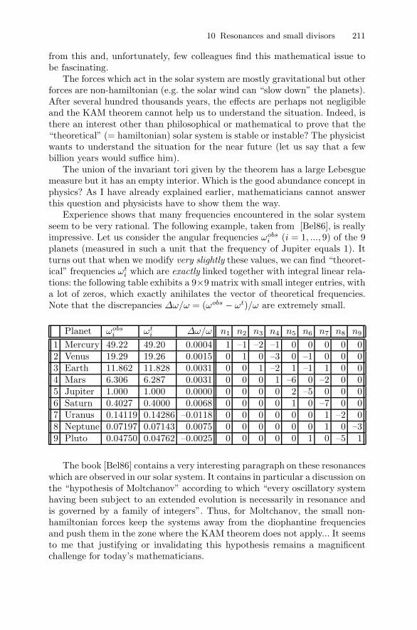
Experience shows that many frequencies encountered in the solar systemseem to be very rational. The following example, taken from [Bel86], is reallyimpressive. Let us consider the angular frequencies ωobsi (i = 1, ..., 9) of the 9planets (measured in such a unit that the frequency of Jupiter equals 1). Itturns out that when we modify very slightly these values, we can find “theoret-ical” frequencies ωti which are exactly linked together with integral linear rela-tions: the following table exhibits a 9×9 matrix with small integer entries, witha lot of zeros, which exactly anihilates the vector of theoretical frequencies.Note that the discrepancies Δω/ω = (ωobs − ωt)/ω are extremely small.

Planet ωobsi ωti Δω/ω n1 n2 n3 n4 n5 n6 n7 n8 n9

1 Mercury 49.22 49.20 0.0004 1 –1 –2 –1 0 0 0 0 02 Venus 19.29 19.26 0.0015 0 1 0 –3 0 –1 0 0 03 Earth 11.862 11.828 0.0031 0 0 1 –2 1 –1 1 0 04 Mars 6.306 6.287 0.0031 0 0 0 1 –6 0 –2 0 05 Jupiter 1.000 1.000 0.0000 0 0 0 0 2 –5 0 0 06 Saturn 0.4027 0.4000 0.0068 0 0 0 0 1 0 –7 0 07 Uranus 0.14119 0.14286 –0.0118 0 0 0 0 0 0 1 –2 08 Neptune 0.07197 0.07143 0.0075 0 0 0 0 0 0 1 0 –39 Pluto 0.04750 0.04762 –0.0025 0 0 0 0 0 1 0 –5 1

The book [Bel86] contains a very interesting paragraph on these resonanceswhich are observed in our solar system. It contains in particular a discussion onthe “hypothesis of Moltchanov” according to which “every oscillatory systemhaving been subject to an extended evolution is necessarily in resonance andis governed by a family of integers”. Thus, for Moltchanov, the small non-hamiltonian forces keep the systems away from the diophantine frequenciesand push them in the zone where the KAM theorem does not apply... It seemsto me that justifying or invalidating this hypothesis remains a magnificentchallenge for today’s mathematicians.

212 Etienne Ghys

References

[AA68] Arnold, V.I., Avez, A.: Ergodic problems of classical mechanics.W. A. Benjamin, Inc., New York-Amsterdam (1968)

[And] http://www-groups.dcs.st-andrews.ac.uk/history, a web site on the his-tory of mathematics.

[Arn63a] Arnold, V.I.: Proof of a theorem of A. N. Kolmogorov on the preserva-tion of conditionally periodic motions under a small perturbation of theHamiltonian (in Russian). Uspekhi Mat. Nauk, 18:F113, 13–40 (1963)

[Arn63b] Arnold, V.I.: Small denominators and problems of stability of motion inclassical and celestial mechanics (in Russian). Uspekhi Mat. Nauk, 18,91–192 (1963)

[Arn83] Arnold, V.I.: Geometric methods in the theory of ordinary differentialequations. Springer, New York (1983)

[Arn89] Arnold, V.I.: Mathematical Methods of Classical Mechanics, 2d ed.Springer (1989)

[Bar97] Barrow-Green, J.: Poincare and the three-body problem. History of Math-ematics, 11. American Mathematical Society, Providence, RI; LondonMathematical Society, London (1997)

[Bel86] Beletski, V.: Essais sur le mouvement des corps cosmiques. Editions Mir,French translation (1986)

[Cop92] Copernicus, N.: On the Revolutions of the Heavenly Bodies, trans.E. Rosen. The Johns Hopkins University Press, Baltimore (1992). Orig-inally published as volume 2 of Nicholas Copernicus’ Complete Works,Jerzy Dobrzycki (Editor), Polish Scientific Publishers, Warsaw (1978)

[Gal01] Gallavotti, G.: Quasi periodic motions from Hipparchus to Kolmogorov.Atti Accad. Naz. Lincei Cl. Sci. Fis. Mat. Natur. Rend. Lincei (9) Mat.Appl., 12, 125–152 (2001)

[Her86] Herman, M.: Sur les courbes invariantes par les diffeomorphismes del’anneau. Asterique, 144 (1986)

[Kol41] Kolmogorov, A.N.: The local structure of turbulence in incompressibleviscous fluid for every large Reynold’s numbers. C. R. (Dokl.) USSR Sci.Acad., 30, 301–305 (1941)

[Kol54] Kolmogorov, A.N.: General theory of dynamical systems and classical me-chanics. In: Proceedings of the International Congress of Mathematicians,Amsterdam, 1954. Erven P. Noordhoff N.V., Groningen (1957)

[Kor89] Korner, T.: Fourier analysis. Cambridge University Press, Cambridge(1989)

[Mos62] Moser, J.: On invariant curves of area-preserving mappings of an annulus.Nachr. Akad. Wiss. Gottingen Math.-Phys. Kl. II, 1–20 (1962)

[Niv56] Niven, I.: Irrational numbers. The Carus Mathematical Monographs,no 11. The Mathematical Association of America. Distributed by JohnWiley and Sons, Inc., New York (1956)

[Pet93] Peterson, I.: Newton’s Clock: Chaos in the Solar System. W. H. Freeman& Co, N.Y. (1993)

[Poi90] Poincare, H.: Sur le probleme des trois corps et les equations de la dy-namique (1890). Œuvres, volume VII, Gauthier-Villars, Paris (1951)

[Ste69] Sternberg, S.: Celestial Mechanics, parts I and II. W.A. Benjamin (1969)


[Yoc06] Yoccoz, J.C.: Une erreur feconde du mathematicien Henri Poincare[A fruitful error by the mathematician Henri Poincare]. Soc. Math. France/ Gazette Math., 107, p. 19–26 (jan. 2006)

[Zee98] Zeeman, C.: Gears from ancient Greeks (1998). The transparencies of thisconference are available at http://www.math.utsa.edu/ecz/

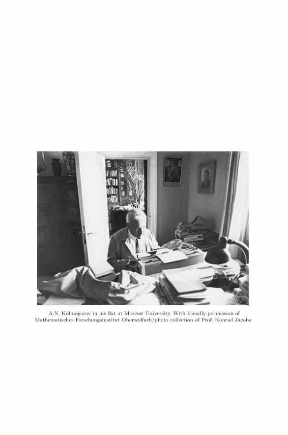
A.N. Kolmogorov in his flat at Moscow University. With friendly permission ofMathematisches Forschungsinstitut Oberwolfach/photo collection of Prof. Konrad Jacobs

Documents

10 Resonances and small divisors