Version SJG/1

EGT2ENGINEERING TRIPOS PART IIA

Friday 22 April 2016 9.30 to 11

Module 3F3

SIGNAL AND PATTERN PROCESSING - SOLUTIONS

Answer not more than three questions.

All questions carry the same number of marks.

The approximate percentage of marks allocated to each part of a question isindicated in the right margin.

Write your candidate number not your name on the cover sheet.

STATIONERY REQUIREMENTSSingle-sided script paper

SPECIAL REQUIREMENTS TO BE SUPPLIED FOR THIS EXAMCUED approved calculator allowed

10 minutes reading time is allowed for this paper.

You may not start to read the questions printed on the subsequentpages of this question paper until instructed to do so.

Page 1 of 16

Version SJG/1

1 Examiner’s comments:

This question was found reasonably straightforward by most, though hardly anyone couldsketch the phase response in part (a)(iii). Similarly in (b)(i) a surprising number ofstudents could not find the 8th roots of unity.

(a) A complex-coefficient digital filter has a transfer function of the following form:

H(z) =z−1− r exp(− jφ)1− z−1r exp( jφ)

(i) Sketch the pole-zero diagram for such a filter when r = 0.7 and φ = π/4. [10%]Solution:1 zero at r−1e jφ . 1 pole at re jφ :

(ii) Determine the frequency response of such a filter for any (r,φ) and showby geometrical arguments from the pole-zero diagram, or otherwise, that allfrequencies are passed with equal gain, i.e. the filter is all-pass. [25%]For frequency response substitute z = e jθ :

H(e jθ ) =e− jθ − r exp(− jφ)1− e− jθ r exp( jφ)

Gain of filter is:

H(e jθ ) =|e− jθ − r exp(− jφ)||1− e− jθ r exp( jφ)|

=|e− jθ − r exp(− jφ)||e jθ − r exp( jφ)|

= L/M = 1,

see diagram:

Page 2 of 16 (cont.

Version SJG/1

(iii) Sketch the phase response of the above filter when r = 0.95 and φ = π/4,for a range of normalised frequencies from 0 to 2π . Your justification shouldbe geometric and based on the pole-zero diagram; you may utilise the fact thatpole/zero pairs are close to each other (and the unit circle) when r = 0.95. [20%]Solution:Use the standard result that phase response is the angle of e jθ − c minus the angleof e jθ −d, where c is the zero of the filter and d is the pole. But note that there isan extra π−φ term since:

H(z) =−r exp(− jφ)(z−1/r exp( jφ))

z− r exp( jφ)=

r exp( j(π−φ))(z−1/r exp( jφ))z− r exp( jφ)

The first observation is that the pole and zero are close together, so that the phasefrom the pole/zero term is nearly zero when we are far from the pole/zero on the unitcircle. Moreover, as we approach θ = φ , the phase sharply decreases by decreasesby 2π:

Page 3 of 16 BAD PAGEBREAK

Version SJG/1

(iv) Explain how a real-coefficient filter can be generated from a combinationof two such structures, retaining the all-pass property but with modified phaseresponse. [10%]Solution:We cascade it with a second all-pass complex filter having pole at r,−θ , henceproviding pole-zero conjugate pairs for the first filter. Thus the coefficients are realbut it is still all-pass.

(b) (i) A second digital filter has the following transfer function:

H(z) =1− z−P

1− rz−P

where 0 < r < 1 and P > 1 is an integer.

A. Sketch the pole-zero diagram for this filter when P = 8 and r = 0.8. [10%]Solution:Poles are at:

rz−P = 1,

i.e.

z = r1/Pei2π p/P, p = 0,1,2, ...

Zeros similarly are at

z = ei2π p/P, p = 0,1,2, ...

Pole-zero diagram:

Page 4 of 16 (cont.

Version SJG/1

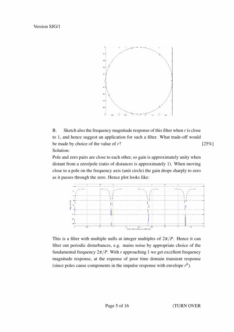
B. Sketch also the frequency magnitude response of this filter when r is closeto 1, and hence suggest an application for such a filter. What trade-off wouldbe made by choice of the value of r? [25%]Solution:Pole and zero pairs are close to each other, so gain is approximately unity whendistant from a zero/pole (ratio of distances is approximately 1). When movingclose to a pole on the frequency axis (unit circle) the gain drops sharply to zeroas it passes through the zero. Hence plot looks like:

This is a filter with multiple nulls at integer multiples of 2π/P. Hence it canfilter out periodic disturbances, e.g. mains noise by appropriate choice of thefundamental frequency 2π/P. With r approaching 1 we get excellent frequencymagnitude response, at the expense of poor time domain transient response(since poles cause components in the impulse response with envelope rk).

Page 5 of 16 (TURN OVER

Version SJG/1

2 Examiner’s comment:

Attempted by nearly all candidates with very good results in general.

The discrete Fourier transform (DFT) of a sequence xn, n = 0,1, ...,N−1 is given by:

Xp =N−1

∑n=0

xne−jnp2π

N

(a) Show that the DFT spectrum values Xp are related to the true DTFT spectrumX(e jθ ) of xn, n =−∞, ...,−1,0,1,2..., ∞, by the following convolution formula:

Xp =1

2π

∫ 2π

0W (e jθ )X(e j(p(2π/N)−θ))dθ

where W (e jθ ) is the DTFT of the appropriate rectangular window function. Whatfrequency, in rads/s would correspond to θ = 0.2, if the digital sampling frequencyis 44.1kHz? [30%]

(b) Explain with the aid of diagrams how the DFT modifies the DTFT spectrum ofa complex exponential signal exp( jω0t) where ω0 is a fixed frequency. Describe theeffects of spectral smearing and spectral leakage, how the use of window functionsmight aid the analysis, and why this is important for analysis of multiple frequencycomponents. [20%]

(c) Show that when N is even, the DFT of a data sequence xn may be expressedin the form:

Xp = Ap +W pBp and Xp+N/2 = Ap−W pBp

where Ap and Bp are DFTs of length N/2 sub-sequences of xn, and W is a suitablecomplex exponential (you should derive the formulae for Ap, Bp and W ). [30%]

(d) Explain briefly how the representation in (c) above allows a very efficientimplementation of the DFT when N is a power of 2. Show that the computationalload, neglecting additions, is approximately (N/2) log2(N) complex multiplicationsand additions. How does this compare with direct evaluation of the DFT? [20%]

SOLUTION:

(a) Consider applying a recangular window wn = 1, n = 0,1, ...,N − 1 to thesignal and xn and take the DTFT:

Xw(e jωT ) =∞

∑n=−∞

{xn wn}e− jnωT

=N−1

∑n=0{xn }e− jnωT

Page 6 of 16 (cont.

Version SJG/1

and clearly this is equal to the DFT when we evaluate at ωp = 2π p/N.Now, proceeding from the first line:

Xw(e jωT ) =∞

∑n=−∞

xp

{1

2π

∫ 2π

0W (e jθ )e jnθ dθ

}e− jnωT

=1

2π

∫ 2π

0W (e jθ )

∞

∑n=−∞

xn e− jn(ωT−θ) dθ

Xw(e jωT ) =1

2π

∫ 2π

0W (e jθ )X(e j(ωT−θ))dθ

and evaluating this at discrete frequencies ωp = p2π/N gives the required result.[Knowledgable students could quote this result directly using the discrete timeconvolution theorem].Now, the frequency at θ = 0.2 is 0.2×44100/2π = 1404Hz.

(b) This is part is standard bookwork. Based on result of part (a) we see thatthe delta-funtions of the pure complex exponentials are convolved with the windowspectrum, leading to spectral smearing and spectral leakage. Window functionsfrom e.g. generalised Hamming families will increase specral smearing but candramatically improve spectral leakage through much lower sidelobe levels. Suitablediagrams from lecture notes are:

Page 7 of 16 BAD PAGEBREAK

Version SJG/1

Page 8 of 16 (cont.

Version SJG/1

(c) First rewrite the DFT equation in terms of the even-indexed and odd-indexeddata xn:

Xp =

N2−1

∑n=0

x2n e− j 2πN (2n)p +

N2−1

∑n=0

x2n+1e− j 2πN (2n+1)p

=

N2−1

∑n=0

x2ne− j 2π

(N/2)np+ e− j 2π

N pN2−1

∑n=0

x2n+1e− j 2π

(N/2)np

= Ap +W pBp (1)

where

Ap =

N2−1

∑n=0

x2ne− j 2π

(N/2)np

Bp =

N2−1

∑n=0

x2n+1e− j 2π

(N/2)np

W = e− j 2πN

Look at the DFT values Xp+N/2:

X p+N/2

=

N2−1

∑n=0

x2n e− j 2π

(N/2)n(p+N/2)

+ e− j 2πN (p+N/2)

N2−1

∑n=0

x2n+1 e− j 2π

(N/2)n(p+N2 )

=

N2−1

∑n=0

x2n e− j 2π

(N/2)np

− e− j 2πN p

N2−1

∑n=0

x2n+1 e− j 2π

(N/2)np

= Ap−W pBp (2)

[Here we have used the results: exp(i(θ + 2π)) = exp(iθ) and exp(i(θ + π)) =

−exp(iθ).]

(d) Repeated application of the above procedure to each of the subsequence DFTssuccessively reduces the computation of the N-DFT to N single point DFTs, withno computational burden. The remaining computations are calculated as follows:

Page 9 of 16 BAD PAGEBREAK

Version SJG/1

•Each stage of the FFT reduces computation by half but introduces an extra N2

multiplications W pBp.

•For N = 2M , the process can be repeated M times to reduce the computation tothat of evaluating N single point DFTs which requires no computation.

•However, at each of the M stages of reduction an extra N2 multiplications are

introduced so that the total number of complex multiplies required to evaluatean N-point DFT is:

N2× (Number of levels) =

N2

log2(N)

Compare with the DFT,which has roughly N2 complex multiplications. We seethat for large N there are very significant savings from use of the FFT.

Page 10 of 16

Version SJG/1

3 Examiner’s comment:

Popular question, with high marks in general. Lots of people did not know how to findaverage energy within a frequency band in part (a). Part (b)(ii) âAS lots of candidatesstated the result for the case when y is stationary, which lost some credit and made part (iii)awkward to demonstrate convincingly. In (b)(iii) many people were careless in checkingthe condition for finite variance and many forgot to check constant mean.

(a) For a discrete-time random process, explain the concept of stationarity andergodicity, and define the terms autocorrelation function, wide-sense stationarityand power spectrum. Show how to obtain the average power of a real-valued processbetween two normalised frequencies ω1 and ω2, with 0≤ ω1 < ω2 < π . [30%]SOLUTION:Stationarity: a process is stationary if the the statistical characteristics centred atone time cannot be distinguished from those at any other time.Ergodicity: an ergodic process ‘forgets’ its initial conditions with time and alwaysconverges on a stationary distribution of values.Autocorrelation function (ACF):

RXX [n,m] = E[XnXm]

Wide-sense stationary (WSS) : ACF depends only on time difference m− n, meanis constant over time, and variance is finite.Power spectrum SX is the DTFT of the ACF for a WSS process.Calculate power as:

2∫

ω2

ω1SX (e

jωT )dω

(b) A random process {yn} is passed through a causal linear system havingimpulse response hm = αm:

zn =+∞

∑m=0

hmyn−m.

(i) Show how the linear system may be implemented as a first-order infiniteimpulse response (IIR) digital filter. [10%]The z-transform of the impulse response is:

11−αz−1

so this can be implemented as

zn = αzn−1 + yn

Page 11 of 16 BAD PAGEBREAK

Version SJG/1

(ii) If {yn} has autocorrelation function E[ykyl ] = RYY [k, l], find anexpression for the cross-correlation function between {yn} and {zn}, and alsothe autocorrelation function of the output process {zn}. [20%]SOLUTION:Note that we haven’t yet stated that {yn} is stationary, so:

RY Z[k, l] = E[ykzl ]

= E[yk

∞

∑m=0

hmyl−m]

= E[∞

∑m=0

hmykyl−m]

=∞

∑m=0

hmRYY [k, l−m] =∞

∑m=0

αmRYY [k, l−m]

RZZ[k, l] = E[zkzl ]

= E[∞

∑n=0

hnyk−n

∞

∑m=0

hmyl−m]

=∞

∑n=0

∞

∑m=0

hnhmRYY [k−n, l−m]

=∞

∑n=0

∞

∑m=0

αn+mRYY [k−n, l−m]

(iii) If {yn} is wide-sense stationary, show that {zn} is also wide-sensestationary, provided the condition |α| < 1 applies. [Hint: the largest value ofthe autocorrelation function is always at lag zero.] [20%]Check mean of {zn}:

E[zn] = E[∞

∑m=0

hmyk−m] =∞

∑m=0

hmµY

which is constant since it does not depend on n.Autocorrelation function:

RZZ [k, l] =∞

∑n=0

∞

∑m=0

αn+mRYY [k−n, l−m] =

∞

∑n=0

∞

∑m=0

αn+mRYY [l−m+n−k]

which depends only on the lag difference l− k, since the n and m variables aresummed out.Check variance of z:

RZZ [k,k] =∞

∑n=0

∞

∑m=0

αn+mRYY [n−m]

Page 12 of 16 (cont.

Version SJG/1

Now, |RYY [n−m]| ≤ RYY [0], since the maximum autocorrelation value is at lag0. Hence:

RZZ[k,k]≤∞

∑n=0

∞

∑m=0|αn+m|RYY [0] =RYY [0]

∞

∑n=0

∞

∑m=0|αn+m|=RYY [0]

∞

∑n=0|αn|

∞

∑m=0|αm|

and both sums are finite only for |α|< 1 - can check by summing GPs.Hence σ2 = RZZ [k,k]− µ2

Z is also finite under the same condition and theprocess is WSS.

(iv) If {yn} is zero-mean white noise with variance 1, and |α|< 1, determinethe power spectrum of {yn}, the autocorrelation function for {zn} and the powerspectrum of {zn}. Sketch the power spectrum SZ(exp( jθ)) for α = 0.8 over therange of normalised frequencies θ = 0 to 2π . [20%]SOLUTION:Power spectrum of {yn} is just flat:

SY (ejθ ) = 1

Easiest way to the power spectrum for {z} is through the frequency domain,and using the filtering result from part (b):

SZ = |H(e jθ )|2SY (ejθ ) =

1|1−αe− jθ |2

though it could also be got as the DTFT of the autocorrelation function.The sketch will look like this, with a resonance at zero and 2π correspondingto the single pole at z = α , i.e. at zero frequency:

The autocorrelation function is:

RZZ [δ ] =∞

∑n=0

∞

∑m=0

αn+mRYY [δ −m+n] = α

δ∞

∑m=0

α2n = α

δ/(1−α2)

Page 13 of 16 (TURN OVER

Version SJG/1

4 Examiner’s comment:

The least popular question, but well handled by most.

Consider the k-means clustering algorithm which seeks to minimise the cost function

C =N

∑n=1

K

∑k=1

snk‖xn−mk‖2

where mk is the mean (centre) of cluster k, xn is data point n, snk = 1 signifies that datapoint n is assigned to cluster k, and there are N data points and K clusters.

(a) Given all the cluster assignments snk (with the constraint that each data pointmust be assigned to one cluster, that is, ∑k snk = 1 for all n, and snk ∈ {0,1} for alln and k), derive the value of the means {mk} which minimise the cost C and give aninterpretation in terms of the k-means algorithm. [30%]

(b) Give an interpretation of the k-means algorithm in terms of a probabilisticmodel. Describe up to three generalisations based on this probabilistic model. [40%]

(c) You are applying the k-means algorithm to a large collection of images, wheremost of the images are not labelled, but you have labels for a few of the images (e.g.“cat”, “dog”, “person”, “car”). You would like to modify your k-means algorithmso that images with the same label are always in the same cluster, and images withdifferent labels are never in the same cluster. Describe a modified version of thealgorithm that would do this. [30%]

SOLUTION

(a) Given the cluster assignments, the problem decomposes into separateminimisations over each mean k, that is, C = ∑k Ck. Since the cluster assignmentsare binary, for each mean we have a cost function

Ck =N

∑n=1

snk‖xn−mk‖2 = ∑n:snk=1

‖xn−mk‖2

Minimising over mk results in

mk =∑n:snk=1 xn

∑n snk

which is simply the Euclidean mean of the data points assigned to cluster k.

(b) The k-means algorithm is closely related to the Gaussian mixture model, aprobabilistic model for density esimation. In fact, the k-means cost is equal up toa constant to the (negative) log likelihood of a Gaussian mixture model under the

Page 14 of 16 (cont.

Version SJG/1

following assumptions: (1) the Gaussians have means mk and covariances that are amultiple of the identity matrix, (2) the Gaussians all have equal mixing proportions,(3) the assignment variables which are actually hidden are treated as parametersand optimised rather than summed out. Upto these three constraints, k-means isalmost identical to the EM algorithm. Once this relationship is established severalgeneralisations become possible: (1) using different covariance matrices for eachcluster to allow for elongated clusters at different orientations, (2) allowing differentmixing proportions so that some clusters can be bigger than others, (3) handlingpartial membership of data points in clusters by accounting for the uncertainty in theassignment variables snk, (4) use of models other than the Gaussian to capture eachcluster (e.g. mixtures of any other distribution), and (5) Bayesian generalisationswhereby the number of clusters can be learned from data, and the uncertaintly inclustering is represented in the inference.

(c) Assume that the number of clusters K is equal or greater than the number oflabels (otherwise the constraints can’t be satisfied). Initalise assignments so that thelabelled images belong to separate clusters (e.g. all “cats” in cluster 1, all “dogs”in cluster 2, etc). Run the k-means algorithm as before on all the unlabelled data,but ensure that the assignments for the labelled data remain unchanged. Since theconstraints are imposed at initialisation and kept at each iteration, this will convergeto a solution which is a (local) minimum of the cost C subject to the imposedconstraints.

END OF PAPER

Page 15 of 16

Version SJG/1

THIS PAGE IS BLANK

Page 16 of 16