10 Inflation

Note: This Chapter is written partly just as an outline, since I am following prettyclosely Chapter 3 of the book by Liddle&Lyth[1]. If you missed my lecture, see theirbook for the discussion.

10.1 Motivation

• Modern view: The most important property of inflation is that it generatesthe initial density fluctuations.

• Historical motivation:

– Whether initial conditions for Big Bang seem natural:

∗ flatness problem

∗ horizon problem

– Unwanted relics:

∗ gravitinos (m ∼ 100 GeV)

∗ magnetic monopoles

– (These are problems in standard Hot Big Bang theory, which are solvedby inflation.)

10.1.1 Flatness problem

Ω − 1 =K

a2H2(1)

If Ω = 1, it stays that way. If Ω 6= 1, it evolves: Ω(t).

mat.dom a ∝ t2/3, H ∝ t−1 ⇒ 1

aH∝ t1/3 ⇒ |1 − Ω| ∝ t2/3 (2)

rad.dom a ∝ t1/2, H ∝ t−1 ⇒ 1

aH∝ t1/2 ⇒ |1 − Ω| ∝ t (3)

(assuming |Ω − 1| is small, i.e., universe not curvature-dominated)

Today: Ω0 = O(1) ⇒ e.g. |Ω(tBBN) − 1| . 10−16

∴ Initial condition: Ω extremely close to 1 — seems unlikely!

Otherwise:

• Ωi > 1 ⇒ recollapse almost immediately

• Ωi < 1 ⇒ blows up fast and cools to T < 3K in less than 1 s

(thus the flatness problem can also be called the oldness problem)

10.1.2 Horizon problem

The horizon problem can also be called the homogeneity problem.Regions on the CMB sky separated by more than about 1 had not had time to

interact, yet their temperature is the same with an accuracy of . 10−4.

∴ The homogeneity must have been an initial condition.

109

10 INFLATION 110

Figure 1: The horizon problem.

10.1.3 Unwanted relics

If the Hot Big Bang begins at very high T it may produce objects surviving to thepresent, that are ruled out by observations.

• Gravitino. The supersymmetric partner of the graviton. m ∼ 100 GeV.They interact very weakly (gravitational strength) ⇒ they decay late, afterBBN, and ruin the success of BBN.

• Magnetic monopoles. If the symmetry of a Grand Unified theory (GUT)is broken in a spontaneous symmetry breaking phase transition, magneticmonopoles are produced. These are point-like topological defects that are stableand very massive, m ∼ TGUT ∼ 1014 GeV. Their expected number density issuch that their contribution to the energy density today ≫ the critical density.

• Other topological defects (cosmic strings, domain walls). These may alsobe produced in a GUT phase transition, and may also be a problem, but thisis model-dependent. On the other hand, cosmic strings have been suggestedas a possible explanation for the initial density perturbations—so they wouldbe beneficial—but this scenario has fallen in trouble with the observationaldata (especially the anisotropy of the CMB).

These relics are produced very early, at extremely high temperatures, typicallyT & 1014 GeV. From BBN, we only know that we should have standard Hot BigBang for T . 1 MeV.

10.1.4 What is needed

∴ We are perfectly happy if we can produce as an “initial condition” for Big Bang auniverse with temperature 1 MeV < T < 1014 GeV, which is almost homogeneous

10 INFLATION 111

and has Ω = 1 with extremely high precision.

10.2 Inflation Introduced

Inflation is not a replacement for the Hot Big Bang, but an add-on to it, occurringat very early times (e.g., t ∼ 10−35 s) without disturbing any of its successes.

Consider how the flatness and horizon problems arise:The origin of the flatness problem is that |Ω − 1| = |K|/(aH)2 grows with time.

Nowd

dt|Ω − 1| = |K| d

dt

(1

a2H2

)

= |K| d

dt

(1

a2

)

=−2|K|

a3a . (4)

For an expanding universe, aH = a(

aa

)= a > 0. Thus a3 > 0, and

d

dt|Ω − 1| > 0 ⇔ a < 0 . (5)

Thus the reason for the flatness problem is that the expansion of the universe isdecelerating, i.e., slowing down. If we had an early period in the history of the uni-verse, where the expansion was accelerating, that could make an initially arbitraryvalue of |Ω − 1| = |K|/(aH)2 very small.

Definition: Inflation = any epoch when the expansion is accelerating.

Inflation ⇔ a > 0 (6)

Consider then the horizon problem. The problem was that in the standard BigBang the horizon at the time of photon decoupling was small compared to the partof the universe we can see today.

In standard Big Bang the universe is radiation-dominated at first and thenturns matter-dominated somewhat before photon decoupling. Thus the horizon atdecoupling, dhor(tdec) is somewhere between the radiation-dominated and matter-dominated values, H−1 and 2H−1. For comparing sizes of regions at different times,we should use there comoving sizes, dc ≡ a0

a d. We have

dchor(tdec) ∼

a0

adecH−1

dec (7)

whereas the size of the observable universe today is of the order of the present Hubblelength

dchor(t0) ∼ H−1

0 . (8)

The horizon problem arises because the first is much smaller than the second,

dchor(tdec)

dchor(t0)

∼ a0H0

adecHdec≪ 1 . (9)

Thus the problem is that aH decreases with time,

d

dt(aH) =

d

dt(a) = a < 0 . (10)

Thus we see, that having a period with a > 0 might solve the problem.

10 INFLATION 112

In the preceding we referred to the (comoving) horizon distance at some time t,defined as the comoving distance light has traveled from the beginning of the universeuntil time t. If there are no surprises at early times, we can calculate or estimate it;like in the preceding where we assumed radiation-dominated or matter-dominatedbehavior (standard Big Bang). If we now start adding other kind of periods, likeaccelerating expansion at early times, the calculation of dhor will depend on them.Now, in principle, we have always dc

hor(t0) > dchor(tdec) since t0 > tdec, and the

interval (0, tdec) is included in the interval (0, t0). But note that in the discussion ofthe horizon problem, the relevant present horizon is how far we can see, and thusthe size of the present observable universe is given just by the integrated comovingdistance the photon has traveled in the interval (tdec, t0), and this is not affected bywhat happens before tdec. Thus the relevant present horizon is still ∼ H−1

0 .What is the relation between dc

hor(t) and (a0/a)H−1 for arbitrary expansionlaws?

To help this discussion we introduce the comoving, or conformal, Hubble param-eter,

H ≡ a

a0H =

1

a

da

dη≡ a

a0, (11)

where η is the conformal time. We will have much use for H in this and laterchapters.

The Hubble length is

lH ≡ H−1 , where H ≡ a

a, (12)

and the comoving Hubble length is

lcH ≡ a0

alH =

a0

aH=

a0

a=

1

H = H−1 (13)

Roughly speaking, the comoving Hubble length gives the comoving distance lighttravels in a “cosmological timescale”, i.e., the Hubble time. This statement cannotbe exact, since both the comoving Hubble length and the Hubble time change withtime. However, if the comoving Hubble length H−1 is increasing with time then itmeans that the comoving distances traveled at earlier “epochs” are shorter, and thusthe comoving Hubble distance at time t, is a good estimate for the total comovingdistance light has traveled since the beginning of time (the horizon). On the otherhand, if H−1 is shrinking, then at earlier epochs light was traveling longer comovingdistances, and we expect the horizon at time t to be larger than H−1.

Thus we have in any case that

dchor(t) & H(t)−1 (14)

Since the Hubble length is more easily “accessible” (less information needed tofigure it out) than the horizon distance it has become customary in cosmology to usethe word “horizon” also for the Hubble distance. We shall also adopt this practice.The Hubble length gives the distance over which we have causal interaction in cos-mological timescales. The comoving Hubble length gives this distance in comovingunits.

If aH is decreasing (Eq. 10) then H−1 increases, and vice versa.

10 INFLATION 113

∴ Inflation = any epoch when the comoving Hubble length is shrinking.

Inflation ⇔ d

dt

(1

H

)

< 0 (15)

Thus the comoving distance over which we have causal connection is decreasingduring inflation. That is, causal contact to other parts of the Universe is being lost.

The preceding can be discussed either 1) in terms of physical distances or 2) interms of comoving distances.

1) In terms of physical distance, the distance between any two points in theUniverse is increasing, with an accelerating rate. The distance over which causalconnection can be maintained is increasing more slowly (typically much more slowly).Therefore causal connection to other parts is lost.

2) In terms of comoving distance, i.e., viewed in comoving coordinates, the dis-tance between to points stays fixed; regions of the universe corresponding to presentstructures maintain fixed size. In this view, the region causally connected to a givenlocation in the Universe is shrinking.

The second Friedmann equation is

a

a= −4πG

3(ρ + 3p) (16)

∴ Inflation ⇔ ρ + 3p < 0 (17)

Thus inflation requires negative pressure, p < −13ρ (we always assume ρ ≥ 0).

Inflation is not so much a theory, than a general idea of a certain kind of behaviorfor the universe. There is a huge class of models which realize this idea. These modelsrely on so-far-unknown physics of very high energies. Some models are just “toymodels”, with a hoped-for resemblance to the actual physics of the early universe.Others are connected to proposed extensions (like supersymmetry) to the standardmodel of particle physics.

The important point is that inflation makes many “generic” predictions, i.e.,predictions that are independent of the particular model of inflation. Present obser-vational data agrees with these predictions. Thus it is widely believed—or consideredprobable—by cosmologists that inflation indeed took place in the very early universe.There are also numerical predictions of cosmological observables that differ from onemodel of inflation to another, allowing future observations to rule out classes of suchmodels. (Some inflation models are already ruled out.)

10.3 Solving the Problems

Inflation can solve1 all the problems discussed in Sec. 10.1. The idea is that duringinflation the universe expands by a large factor (at least by a linear factor of ∼ e70

1This is not to be taken too rigorously. The problems are related to the question of initialconditions of the universe at some very early time, whose physics we do not understand. Thustheorists are free to have different views on what kind of initial conditions are “natural”. Inflationmakes the flatness and horizon problems “exponentially smaller” in some sense, but inflation stillplaces requirements—on the level of homogeneity—for the initial conditions before inflation, so thatinflation can begin.

10 INFLATION 114

Figure 2: Solving the flatness problem. This figure is for a universe with no dark energy,where the expansion keeps decelerating after inflation ended in the early universe. Presentobservational evidence indicates that actually the expansion began accelerating again (sup-posedly due to the mysterious dark energy) a few billion years ago. Thus the universe is,technically speaking, inflating again, and Ω is again being driven towards 1. However, thiscurrent epoch of inflation is not enough to solve the flatness problem, or the other problems,since the universe has only expanded by about a factor of 2 during it.

to solve the problems). This expansion cools the universe to T ∼ 0 (if the concept oftemperature is applicable). When inflation ends, the universe is reheated to a hightemperature, and the usual Hot Big Bang history follows.

10.3.1 Solving the flatness problem

The flatness problem is solved, since during inflation

|1 − Ω| =|K|H2

is shrinking. (18)

Thus inflation drives Ω → 1.

Starting with an arbitrary Ω, inflation drives |1 − Ω| so small, that although ithas grown ever since the end of inflation, it is still very small today. See Fig. 2.

In fact, inflation predicts that Ω0 = 1 to extremely high accuracy.2

10.3.2 Solving the horizon problem

The horizon problem is solved, since during inflation the causally connected region isshrinking.3 It was very large before inflation; much larger than the present horizon.Thus the present observable universe has evolved from a small patch of a much largercausally connected region; and it is natural that the conditions were (or became)homogeneous in that patch then. See Fig. 3

2Thus, if it were discovered by observations, that actually Ω0 6= 1, this would be a blow tothe credibility of inflation. However, there is a version of inflation, called open inflation, for whichit is natural that Ω0 < 1. The existence of such models of inflation have led critics of inflationto complain that inflation is “unfalsifiable”—no matter what the observation, there is a modelof inflation that agrees with it. Nevertheless, most models of inflation give the same “generic”

10 INFLATION 115

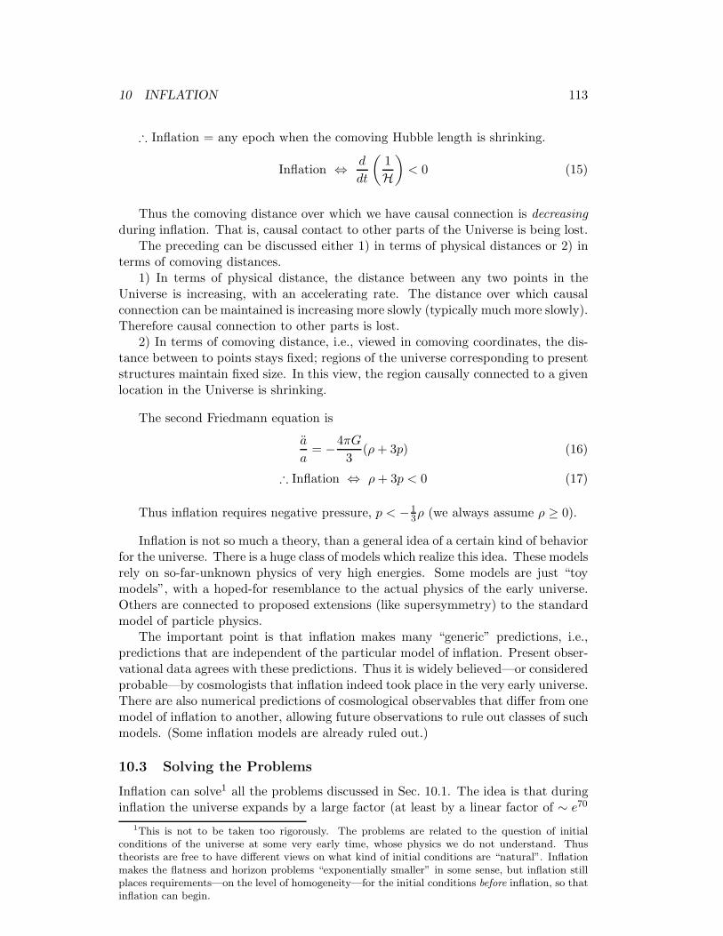
Figure 3: Evolution of the comoving Hubble radius (length, distance) during and afterinflation (schematic).

10.3.3 Getting rid of relics

If unwanted relics are produced before inflation, they are diluted to practically zerodensity by the huge expansion during inflation. We just have to take care they arenot produced after inflation, i.e., the reheating temperature has to be low enough.This is an important constraint on models of inflation.

10.3.4 Forget these now

Actually the question of solving the flatness and horizon problems is more compli-cated. We have only discussed them in terms of a FRW universe, which by assump-tion is already homogeneous. In fact, for inflation to get started, a sufficiently largeregion which is not too inhomogeneous and not too curved, is needed. We shallnot discuss this in any more detail, since the solution of these problems is not themost important aspect of inflation. (The most important aspect is how inflationgenerates the “seeds” for structure formation, which we shall discuss in the Chapteron Structure Formation.)

Thus we assume, that sufficient inflation has already taken place to make theuniverse (within a horizon volume) flat and homogeneous, and follow the inflationin detail after that. Thus we shall work in the flat FRW universe.

predictions, including Ω0 = 1.3We are adopting here the second viewpoint of Sec. 10.2. You should get used to this comoving

viewpoint, since cosmologists tend to use it without warning.

10 INFLATION 116

10.4 Inflaton Field

As we saw in Sec. 10.2, inflation requires negative pressure. In Chapter 5 we con-sidered systems of particles where interaction energies can be neglected (ideal gasapproximation). For such systems the pressure is always nonnegative. However,negative pressure is possible in systems with attractive interactions. In the field pic-ture, negative pressure comes from the potential term. In many models of inflation,the inflation is caused by a scalar field. This scalar field (and the correspondingspin-0 particle) is called the inflaton. We already discussed the pressure and energydensity of a scalar field in the chapter on Quantum Field Theory.

A historical note. The idea of scalar fields playing an important role in thevery early universe was very natural at the time inflation was proposed by AlanGuth[2]. We already mentioned how a scalar field, the Higgs field, is responsiblefor the electroweak phase transition at T ∼ 100 GeV. It is thought that at a muchhigher temperature, T ∼ 1014 GeV, another spontaneous symmetry breaking phasetransition occurred, the GUT (Grand Unified Theory) phase transition, so thatabove this temperature the strong and electroweak forces were unified. This GUTphase transition gives rise to the monopole problem. Guth realized that the Higgsfield associated with the GUT transition might lead the universe to “inflate” (theterm was coined by Guth), solving this monopole problem. It was soon found out,however, that inflation based on the GUT Higgs field is not a viable inflation model,since in this model too strong inhomogeneities were created. So the inflaton fieldmust be some other scalar field. The supersymmetric extensions of the standardmodel contain many inflaton field candidates.

During inflation the inflaton field is almost homogeneous.4 The energy densityand pressure of the inflaton are thus those of a homogeneous scalar field,

ρ =1

2ϕ2 + V (ϕ)

p =1

2ϕ2 − V (ϕ) .

(19)

We can see that negative pressures are quite possible. Usually it is assumed thatV (ϕ) is nonnegative, so that we don’t get negative energy densities. For the equation-of-state parameter w ≡ p/ρ we have

w =ϕ2 − 2V (ϕ)

ϕ2 + 2V (ϕ)=

1 − (2V/ϕ2)

1 + (2V/ϕ2), (20)

so that−1 ≤ w ≤ 1 . (21)

If the kinetic term ϕ2 dominates, w ≈ 1; if the potential term V (ϕ) dominates,w ≈ −1.

For the present discussion, the potential V (ϕ) is some arbitrary function. Differ-ent inflaton models correspond to different V (ϕ). From Eq. (19), we get the usefulcombinations

ρ + p = ϕ2

ρ + 3p = 2[ϕ2 − V (ϕ)

].

(22)

4Inflation makes the inflaton field homogenous. Again, a sufficient level of initial homogeneityof the field is required to get inflation started. We start our discussion when a sufficient level ofinflation has already taken place to make the gradients negligible.

10 INFLATION 117

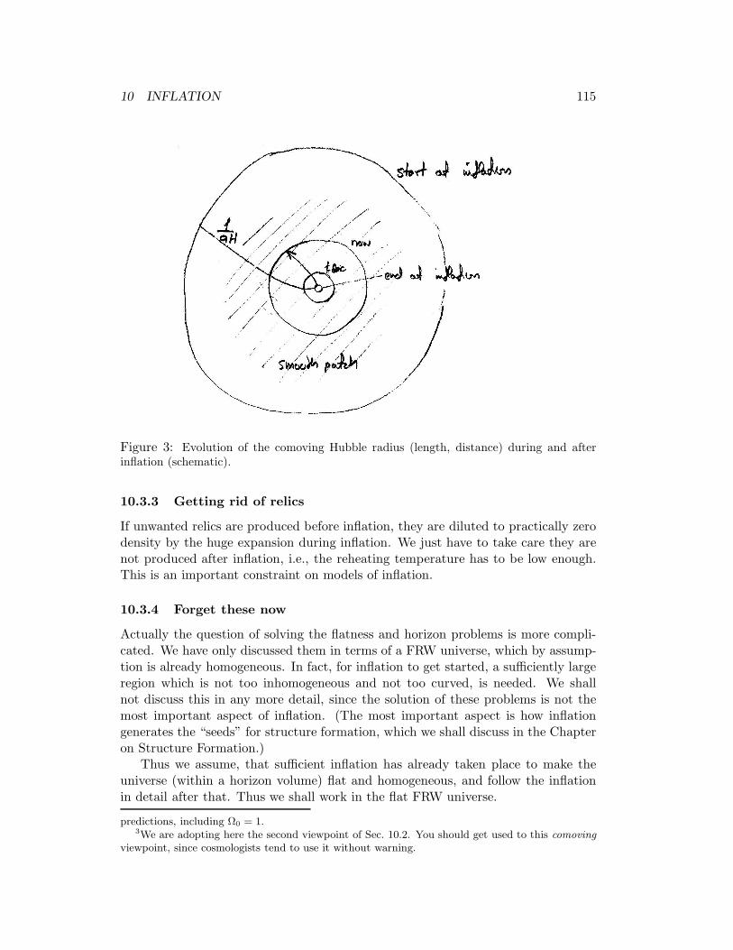
Figure 4: The inflaton and its potential.

We already had the field equation for a scalar field in Minkowski space,

ϕ −∇2ϕ = −V ′(ϕ) . (23)

For the homogenous case it is just

ϕ = −V ′(ϕ) . (24)

We need to modify this for the expanding universe. We do not need to go to theGR formulation of field theory, since the modification for the present case can besimply obtained by sticking the ρ and p of the inflaton field from Eq. (19) into theenergy continuity equation

ρ = −3H(ρ + p) . (25)

This gives

ϕϕ + V ′(ϕ)ϕ = −3Hϕ2 ⇒ ϕ + 3Hϕ = −V ′(ϕ) , (26)

the field equation for a homogeneous ϕ in an expanding (FRW) universe. We seethat the effect of expansion is to add the term 3Hϕ, which acts like a friction term,slowing down the evolution of ϕ.

The condition for inflation, ρ + 3p = 2ϕ2 − 2V (ϕ) < 0, is satisfied, if

ϕ2 < V (ϕ) . (27)

The idea of inflation is that ϕ is initially far from the minimum of V (ϕ). Thepotential then pulls ϕ towards the minimum. See Fig. 4. If the potential has asuitable (sufficiently flat) shape, the friction term soon makes ϕ small enough tosatisfy Eq. (27), even if it was not satisfied initially.

We shall also need the Friedmann equation for the flat universe,

H2 =8πG

3ρ =

1

3M2Pl

ρ . (28)

where we have introduced the reduced Planck mass

MPl ≡1√8π

mPl ≡1√8πG

= 2.436 × 1018 GeV . (29)

Inserting Eq. (19), this becomes

H2 =1

3M2Pl

[1

2ϕ2 + V (ϕ)

]

. (30)

10 INFLATION 118

We have ignored other components to energy density and pressure besides theinflaton. During inflation, the inflaton ϕ moves slowly, so that the inflaton energydensity, which is dominated by V (ϕ) also changes slowly. If there are matter andradiation components to the energy density, they decrease fast, ρ ∝ a−3 or ∝ a−4

and soon become negligible. Again, this puts some initial conditions for inflation toget started, for the inflaton to become dominant. But once inflation gets started,we can soon forget the other components to the universe besides the inflaton.

10.5 Slow-Roll Inflation

The friction (expansion) term tends to slow the evolution of ϕ down, so that we mayeasily reach a situation where:

ϕ2 ≪ V (ϕ) (31)

|ϕ| ≪ |3Hϕ| (32)

These are the slow-roll conditions.If the slow-roll conditions are valid, we may approximate (the slow-roll approxi-

mation) Eqs. (30) and (26) by the slow-roll equations:

H2 =V (ϕ)

3M2Pl

(33)

3Hϕ = −V ′(ϕ) (34)

The shape of the potential V (ϕ) determines the slow-roll parameters:

ε(ϕ) ≡ 1

2M2

Pl

(V ′

V

)2

(35)

η(ϕ) ≡ M2Pl

V ′′

V(36)

Exercise: Show that

ε ≪ 1 and |η| ≪ 1 ⇐ Eqs. (31) and (32) (37)

Note that the implication goes only in this direction. The conditions ε ≪ 1 and|η| ≪ 1 are necessary, but not sufficient for the slow-roll approximation (i.e., theslow-roll conditions) to be valid.

The conditions ε ≪ 1 and |η| ≪ 1 are just conditions on the shape of thepotential, and identify from the potential a slow-roll section, where the slow-rollapproximation may be valid. Since the initial field equation, Eq. (26) was secondorder, it accepts arbitrary ϕ and ϕ as initial conditions. Thus Eqs. (31) and (32)may not hold initially, even if ϕ is in the slow-roll section. However, it turns outthat the slow-roll solution, the solution of the slow-roll equations (33) and (34), isan attractor of the full equations, (30) and (26). This means that the solution of thefull equations rapidly approaches it, starting from arbitrary initial conditions. Well,not fully arbitrary, the initial conditions need to lie in the basin of attraction, fromwhich they are then attracted into the attractor. To be in the basin of attraction,means that ϕ must be in the slow-roll section, and that if ϕ is very large, ϕ needsto be a little deeper in the slow-roll section.

10 INFLATION 119

Figure 5: The potential V (ϕ) = 1

2m2ϕ2 and its two slow-roll sections.

Note that once we have reached the attractor, where Eqs. (33) and (34) hold, ϕis determined by ϕ. In fact everything is determined by ϕ (assuming a known formof the potential V (ϕ)). The value of ϕ is the single parameter describing the stateof the universe, and ϕ evolves down the potential V (ϕ) as specified by the slow-rollequations.

This language of “attractor” and “basin of attraction” can be taken further. Ifthe universe (or a region of it) finds itself initially (or enters) the basin of attractionof slow-roll inflation, meaning that: there is a sufficiently large region, where thecurvature is sufficiently small, the inflaton makes a sufficient contribution to thetotal energy density, the inflaton is sufficiently homogeneous, and lies sufficientlydeep in the slow-roll section, then this region begins inflating, it becomes rapidlyvery homogeneous and flat, all other contributions to the energy density besides theinflaton become negligible, and the inflaton begins to follow the slow-roll solution.

Thus inflation erases all memory of the initial conditions, and we can predictthe later history of the universe just from the shape of V (ϕ) and the assumptionthat ϕ started out far enough in the slow-roll part of it.

Example: (See Fig. 5.)

V (ϕ) =1

2m2ϕ2 ⇒ V ′(ϕ) = m2ϕ , V ′′(ϕ) = m2 (38)

ε(ϕ) =1

2M2

Pl

(2

ϕ

)2

η(ϕ) = M2Pl

2

ϕ2

⇒ ε = η = 2

(MPl

ϕ

)2

(39)

and

ε, η ≪ 1 ⇒ ϕ2 ≫ 2M2Pl (40)

10 INFLATION 120

10.5.1 Relation between Inflation and Slow Roll

H =a

a⇒ H =

a

a− a2

a2⇒ a

a= H + H2 (41)

Thus the condition for inflation is H + H2 > 0.

This would be satisfied, if H > 0, but this is not possible here, since it wouldrequire p < −ρ, i.e., w ≡ p/ρ < −1, which is not allowed by Eq. (19).5

Thus H ≤ 0.

∴ The condition for inflation is−H

H2< 1 (42)

If the slow-roll apx is valid,

H2 =V

3M2Pl

⇒ 2HH =V ′ϕ

3M2Pl

⇒ H2H =V ′Hϕ

6M2Pl

3Hϕ=−V ′

= − V ′2

18M2Pl

⇒ − H

H2=

V ′2

18M2Pl

9M4Pl

V 2=

1

2M2

Pl

(V ′

V

)2

= ε ≪ 1

∴ If the slow-roll apx is valid, inflation is guaranteed.(sufficient, but not necessary condition)

In practice, very little inflation takes place when the slow-roll apx is not valid.

The above result for slow-roll inflation, −H/H2 ≪ 1 can also be written as

∣∣∣∣∣

H

H

∣∣∣∣∣≪ a

a.

Thus, during slow-roll inflation, the Hubble parameter H changes much more slowlythan the scale factor a.

5From the Friedmann eqs.,

„

a

a

«2

=8πG

3ρ −

K

a2

a

a= −

4πG

3(ρ + 3p)

9

>

>

=

>

>

;

⇒ H =a

a−

a2

a2= −4πG

„

ρ + p −K

3a2

«

Thus H > 0 requires ρ + p − K3a2 < 0. In the above, we are assuming space is already flat, i.e., we

can take K = 0

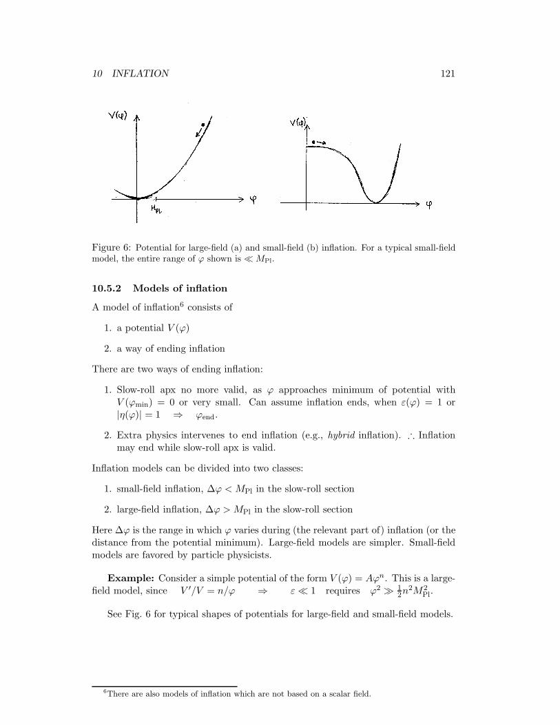
10 INFLATION 121

Figure 6: Potential for large-field (a) and small-field (b) inflation. For a typical small-fieldmodel, the entire range of ϕ shown is ≪ MPl.

10.5.2 Models of inflation

A model of inflation6 consists of

1. a potential V (ϕ)

2. a way of ending inflation

There are two ways of ending inflation:

1. Slow-roll apx no more valid, as ϕ approaches minimum of potential withV (ϕmin) = 0 or very small. Can assume inflation ends, when ε(ϕ) = 1 or|η(ϕ)| = 1 ⇒ ϕend.

2. Extra physics intervenes to end inflation (e.g., hybrid inflation). ∴ Inflationmay end while slow-roll apx is valid.

Inflation models can be divided into two classes:

1. small-field inflation, ∆ϕ < MPl in the slow-roll section

2. large-field inflation, ∆ϕ > MPl in the slow-roll section

Here ∆ϕ is the range in which ϕ varies during (the relevant part of) inflation (or thedistance from the potential minimum). Large-field models are simpler. Small-fieldmodels are favored by particle physicists.

Example: Consider a simple potential of the form V (ϕ) = Aϕn. This is a large-field model, since V ′/V = n/ϕ ⇒ ε ≪ 1 requires ϕ2 ≫ 1

2n2M2Pl.

See Fig. 6 for typical shapes of potentials for large-field and small-field models.

6There are also models of inflation which are not based on a scalar field.

10 INFLATION 122

Figure 7: Remaining number of e-foldings N(t) as a function of time.

10.5.3 Amount of Inflation

During inflation, the scale factor a(t) grows by a huge factor.

Define the number of e-foldings from time t to end of inflation (tend)

N(t) ≡ lna(tend)

a(t)(43)

See Fig. 7.

To solve the horizon and flatness problems, requires N & 70.

As we saw in Sec. 10.5.1, a(t) changes much faster than H(t) (when the slow-rollapproximation is valid), so that the comoving Hubble length H−1 = a0/aH shrinksby almost as many e-foldings. (a(t) grows fast, H(t) decreases slowly.)

We can calculate N(t) ≡ N(ϕ(t)) ≡ N(ϕ) from the shape of the potential V (ϕ)and the value of ϕ at time t:

a = Ha ⇒ da

a= d ln a = Hdt , where dt =

dϕ

ϕ

⇒ N(ϕ) ≡ lna(tend)

a(t)=

∫ tend

tH(t)dt =

∫ ϕend

ϕ

H

ϕdϕ

slow roll≈ 1

M2Pl

∫ ϕ

ϕend

V

V ′dϕ .

(44)

10 INFLATION 123

10.5.4 Evolution of Scales

When discussing (next chapter) evolution of density perturbations and formation ofstructure in the universe, we will be interested in the history of each comoving dis-tance scale, or each comoving wave number k (from a Fourier expansion in comovingcoordinates).

k =2π

λ, k−1 =

λ

2π

An important question is, whether a distance scale is larger or smaller than theHubble length at a given time.

We define a scale to be

• superhorizon, when k < H(k−1 > H−1

)

• at horizon (exiting or entering horizon), when k = H

• subhorizon, when k > H(k−1 < H−1

)

Note that large scales (large k−1) correspond to small k, and vice versa, although weoften talk about “scale k”. This can easily cause confusion, so watch for this, andbe careful in your wording! Notice also, that we are here using the word “horizon”to refer to the Hubble length.7

Inflation ⇒ H−1 shrinking

All other times ⇒ H−1 growing

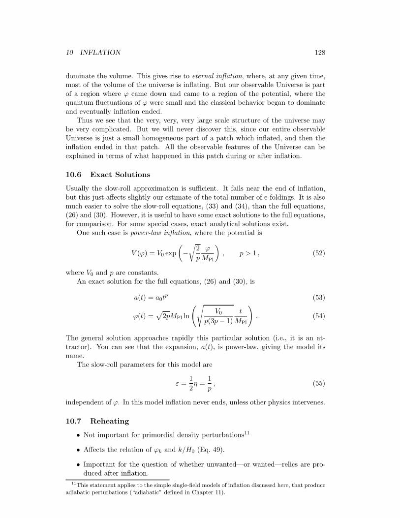
See Figs. 8 and 9.We shall later find that primordial density perturbations are generated for a given

comoving scale as this scale exits the horizon during inflation. The largest observablescales are “at horizon” today. (Since the universe has recently began acceleratingagain, these scales have just barely entered, and are actually now exiting again.)

To identify the distance scales during inflation with the corresponding distancescales in the present universe, we need a complete history from inflation to thepresent.

Divide it into the following periods:

1. From the time the scale k of interest exits the horizon during inflation to theend of inflation (tk to tend).

2. From the end of inflation to the time when thermal equilibrium at high tem-perature (Hot Big Bang conditions) is achieved. This is called reheating.8

Assume (we justify this later, in Sec. 10.7.1) the universe behaves as if matter-dominated, ρ ∝ a−3, during this period (tend to treh).

7There are three different usages for the word “horizon”:

1. particle horizon

2. event horizon

3. Hubble length

8Although it is not clear whether the universe has been “hot”, i.e., in thermal equilibrium, before.

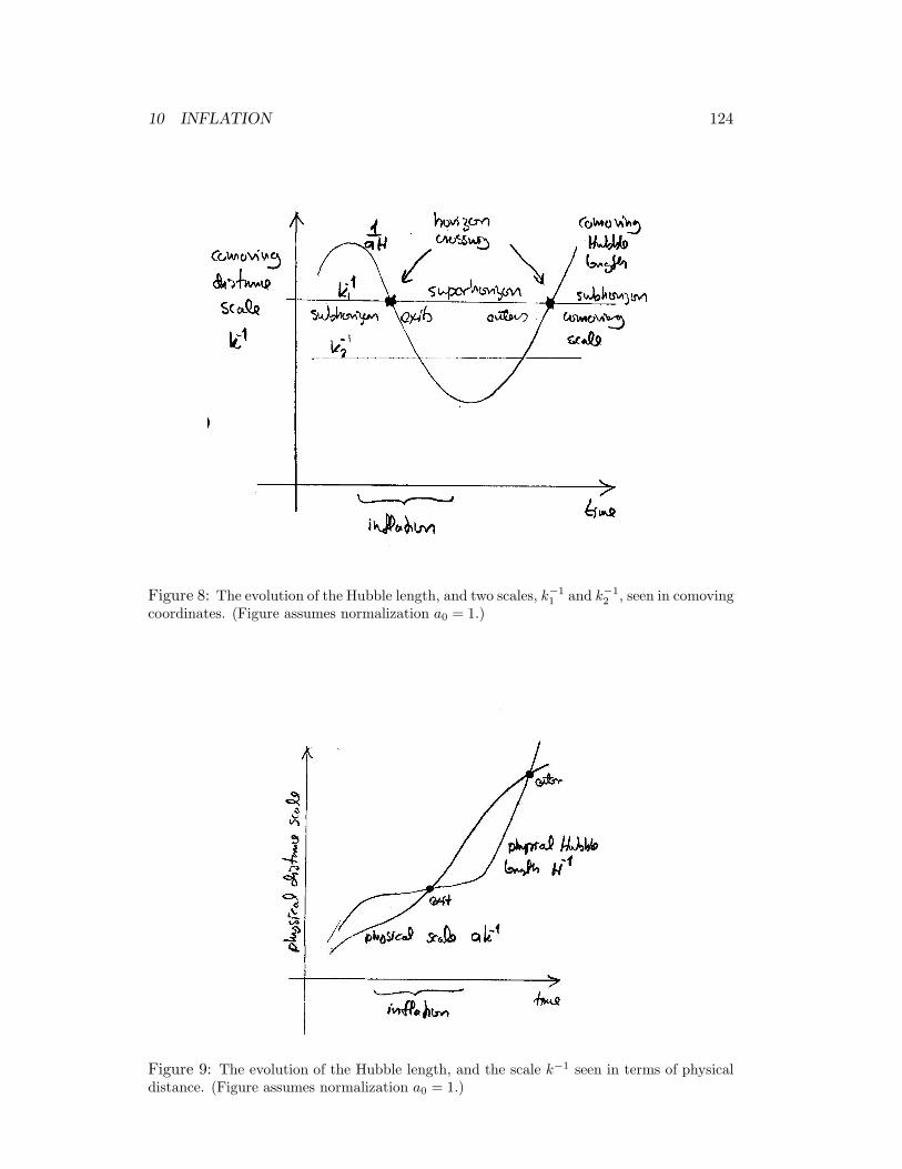
10 INFLATION 124

Figure 8: The evolution of the Hubble length, and two scales, k−1

1and k−1

2, seen in comoving

coordinates. (Figure assumes normalization a0 = 1.)

Figure 9: The evolution of the Hubble length, and the scale k−1 seen in terms of physicaldistance. (Figure assumes normalization a0 = 1.)

10 INFLATION 125

3. From reheating to matter-radiation equality (the radiation era, ρ ∝ a−4, trehto teq).

4. The matter era, ρ ∝ a−3 from teq to t0.

Consider now some scale k, which exits at t = tk, when a = ak and H = Hk

⇒ k = Hk =ak

a0Hk .

To find out how large this scale is today, we relate it to the present “horizon”, i.e.,the Hubble scale:

k

H0=

akHk

a0H0=

ak

aend

aend

areh

areh

aeq

aeq

a0

Hk

H0. (45)

Hereak

aend= e−N(k) ,

where N(k) ≡ number of e-foldings after the scale k exits. We denote the value ofϕ at this moment by ϕk ≡ ϕ(tk), and Vk ≡ V (ϕk). We already found (Eq. 44) that

N(k) ≡ N(ϕk) ≈ 1

M2Pl

∫ ϕk

ϕend

V

V ′dϕ ,

which allows us to relate ϕk to N(k).The factor (areh/aeq)(aeq/a0) is related to the change in energy density from

treh → teq → t0:

treh → teq : ρ ∝ a−4 ⇒ areh

aeq=

(ρeq

ρreh

) 1

4

teq → t0 : ρ ∝ a−3 ⇒ aeq

a0=

(ρ0

ρeq

) 1

3

(where ρ and ρ0 do not include dark energy). We can do this in one step by consid-ering just the present radiation density ρr0:

treh → t0 : ρr ∝ a−4 ⇒ areh

a0=

(ρr0

ρreh

) 1

4

. (46)

This is slightly inaccurate, since ρr ∝ a−4 does not take into account the change ing∗. However, the approximation (46) is good enough9 for us—we are making othercomparable approximations also.

9Accurately this would go as:

g∗sa3T 3 = const. ⇒

areh

a0

=

»

g∗s(T0)

g∗s(Treh)

– 1

3 T0

Treh

(47)

Eq. (46) approximates this with

„

ρr0

ρreh

« 1

4

=

»

g∗(T0)

g∗(Treh)

– 1

4 T0

Treh

Taking g∗s(Treh) = g∗(Treh) ∼ 100, the ratio of these two becomes

(47)

(46)=

g∗s(T0)1

3

g∗(T0)1

4 g∗(Treh)1

12

≈3.909

1

3

3.3631

4 1001

12

= 0.79 ∼ 1

10 INFLATION 126

From end of inflation to reheating

ρ ∝ a−3 ⇒ aend

areh=

(ρreh

ρend

) 1

3

The ratio Hk/H0 we get from

Hk =

√

8πG

3ρk , H0 =

√

8πG

3ρc ⇒ Hk

H0=

(ρk

ρc

) 1

2

,

where ρk is the energy density when scale k exits.Thus we get that

k

H0= e−N(k)

(ρreh

ρend

) 1

3

(ρr0

ρreh

)1

4

(ρk

ρc

)1

2

= e−N(k)

(ρreh

ρend

)1/12( ρk

ρend

)1/4 ρ1/4k ρ

1/4r0

ρ1/2c

.

During inflation ρ = 12 ϕ2 + V (ϕ), where 1

2 ϕ2 ≪ V (ϕ) during slow roll. Thus we cantake ρk ≈ Vk.

We can now relate N(k) to k/H0 as

N(k) = − lnk

H0− 1

3ln

ρ1/4end

ρ1/4reh

+ lnV

1/4k

ρ1/4end

+ lnV

1/4k

1016 GeV+ ln

1016 GeV · ρ1/4r0

ρ1/2c

, (48)

where 1016 GeV serves as a reference scale for Vk. Sticking in the known values

of ρ1/4r0 = 2.375 × 10−13 GeV (includes relativistic neutrinos) and ρ

1/4c = 3.000 ×

10−12 GeV · h1/2, the last term becomes 60.85 − lnh.Thus we get as our final result

N(ϕk) = − lnk

H0+ (60.85 − ln h) − 1

3ln

ρ1/4end

ρ1/4reh

+ lnV

1/4k

ρ1/4end

+ lnV

1/4k

1016 GeV. (49)

For any given present scale, given as a fraction of the present Hubble distance,10

this equation identifies the value ϕk the inflaton had, when this scale exited thehorizon during inflation. The last three terms give the dependence on the energyscales connected with inflation and reheating. In typical inflation models, they arerelatively small. Usually, the precise value of N is not that important; we are more

interested in the derivative dN/dk, or rather dϕk/dk. The V1/4k depends on the

scale k, but since during inflation, V (ϕ) changes slowly, this dependence is weakcompared to the ln k/H0 term.

Anyway, we can see that typically about 60 e-foldings of inflation occur after thelargest observable scales exit the horizon.

Note that a ∝ ρ−1/4

r is a better approximation than a ∝ T−1, since these two differ by

»

g∗(Treh)

g∗(T0)

– 1

4

∼

„

100

3.363

« 1

4

∼ 2.33 .

10For example, k/H0 = 10 means that we are talking about a a scale corresponding to a wave-length λ, where λ/2π is one tenth of the Hubble distance.

10 INFLATION 127

Figure 10: Spacetime foam and some regions emerging from it.

10.5.5 Initial Conditions for Inflation

As we discussed earlier, inflation erases all memory of the initial conditions beforeinflation. However, a complete picture of the history of the universe should alsoinclude some idea about the conditions before inflation. To weigh how plausibleinflation is as an explanation we should be able to contemplate how easy it is forthe universe to begin inflating.

Although inflation differs radically from the other periods of the history of theuniverse we have discussed, two qualitative features still hold true also during infla-tion: 1) the universe is expanding (fast during inflation) and 2) the energy densityis decreasing (slowly during inflation).

Thus the energy density should be higher before inflation than during it or afterit. Often it is assumed that inflation begins right at the Planck scale, ρ ∼ M4

Pl,which is the limit to how high energy densities we can extend our discussion, whichis based on classical GR. When ρ > M4

Pl, quantum gravitational effects should beimportant. We can imagine that the universe at that time, the Planck era, is somekind of “spacetime foam”, where the fabric of spacetime itself is subject to largequantum fluctuations. When the energy density of some region, larger than H−1,falls below M4

Pl, spacetime in that region begins to behave in a classical manner.See Fig. 10.

The initial conditions, i.e, conditions at the time when our Universe emergesfrom the spacetime foam, are usually assumed chaotic (term due to Linde, does notrefer to chaos theory) , i.e., ϕ takes different, random, values at different regions.Since ρ ≥ ρϕ, and

ρϕ =1

2ϕ2 +

1

2∇ϕ2 + V (ϕ) , (50)

we must haveϕ2 . M4

Pl , ∇ϕ2 . M4Pl , V (ϕ) . M4

Pl (51)

in a region for it to emerge from the spacetime foam.Inflation may begin at many different parts of the spacetime foam. Our observ-

able universe is just one small part of one such region which has inflated to a hugesize.

It is also possible that during inflation, for some part of the potential, quantumfluctuations of the inflaton (not of the spacetime) dominate over the classical evolu-tion, pushing ϕ higher in some regions. These regions will then expand faster, and

10 INFLATION 128

dominate the volume. This gives rise to eternal inflation, where, at any given time,most of the volume of the universe is inflating. But our observable Universe is partof a region where ϕ came down and came to a region of the potential, where thequantum fluctuations of ϕ were small and the classical behavior began to dominateand eventually inflation ended.

Thus we see that the very, very, very large scale structure of the universe maybe very complicated. But we will never discover this, since our entire observableUniverse is just a small homogeneous part of a patch which inflated, and then theinflation ended in that patch. All the observable features of the Universe can beexplained in terms of what happened in this patch during or after inflation.

10.6 Exact Solutions

Usually the slow-roll approximation is sufficient. It fails near the end of inflation,but this just affects slightly our estimate of the total number of e-foldings. It is alsomuch easier to solve the slow-roll equations, (33) and (34), than the full equations,(26) and (30). However, it is useful to have some exact solutions to the full equations,for comparison. For some special cases, exact analytical solutions exist.

One such case is power-law inflation, where the potential is

V (ϕ) = V0 exp

(

−√

2

p

ϕ

MPl

)

, p > 1 , (52)

where V0 and p are constants.An exact solution for the full equations, (26) and (30), is

a(t) = a0tp (53)

ϕ(t) =√

2pMPl ln

(√

V0

p(3p − 1)

t

MPl

)

. (54)

The general solution approaches rapidly this particular solution (i.e., it is an at-tractor). You can see that the expansion, a(t), is power-law, giving the model itsname.

The slow-roll parameters for this model are

ε =1

2η =

1

p, (55)

independent of ϕ. In this model inflation never ends, unless other physics intervenes.

10.7 Reheating

• Not important for primordial density perturbations11

• Affects the relation of ϕk and k/H0 (Eq. 49).

• Important for the question of whether unwanted—or wanted—relics are pro-duced after inflation.

11This statement applies to the simple single-field models of inflation discussed here, that produceadiabatic perturbations (“adiabatic” defined in Chapter 11).

10 INFLATION 129

Figure 11: After inflation, the inflaton field is left oscillating at the bottom.

During inflation, practically all the energy in the universe is in the inflatonpotential V (ϕ), since the slow-roll apx says 1

2 ϕ2 ≪ V (ϕ). As inflation ends, thisenergy is transferred in the reheating process to a thermal bath of particles producedin the reheating. Thus reheating creates, from V (ϕ), all the stuff there is in the lateruniverse!

10.7.1 Scalar Field Oscillations

After inflation, the inflaton field ϕ begins to oscillate at the bottom of the potentialV (ϕ), see Fig. 11. The inflaton field is still homogeneous, ϕ(t, ~x) = ϕ(t), so itoscillates in the same phase everywhere (we say the oscillation is coherent). Theexpansion time scale H−1 soon becomes much longer than the oscillation period.

Assume the potential can be approximated as ∝ ϕ2 near the minimum of V (ϕ),so that we have a harmonic oscillator. Write V (ϕ) = 1

2m2ϕ2:

ϕ + 3Hϕ = −V ′(ϕ)

ρ =1

2ϕ2 + V (ϕ)

become

ϕ + 3Hϕ = −m2ϕ

ρ =1

2

(ϕ2 + m2ϕ2

)

What is ρ(t)?

ρ + 3Hρ = ϕ

−3Hϕ︷ ︸︸ ︷(ϕ + m2ϕ

)+3H · 1

2

(ϕ2 + m2ϕ2

)=

3

2H

oscillates︷ ︸︸ ︷(m2ϕ2 − ϕ2

)

The oscillating factor on the right hand side averages to zero over one oscillationperiod (in the limit where the period is ≪ H−1).

∴ Averaging over the oscillations, we get that the long-time behavior of theenergy density is

ρ + 3Hρ = 0 ⇒ ρ ∝ a−3 , (56)

just like in a matter-dominated universe (we used this result in Sec. 10.5.4). The fallin the energy density shows as a decrease of the oscillation amplitude, see Fig. 12.

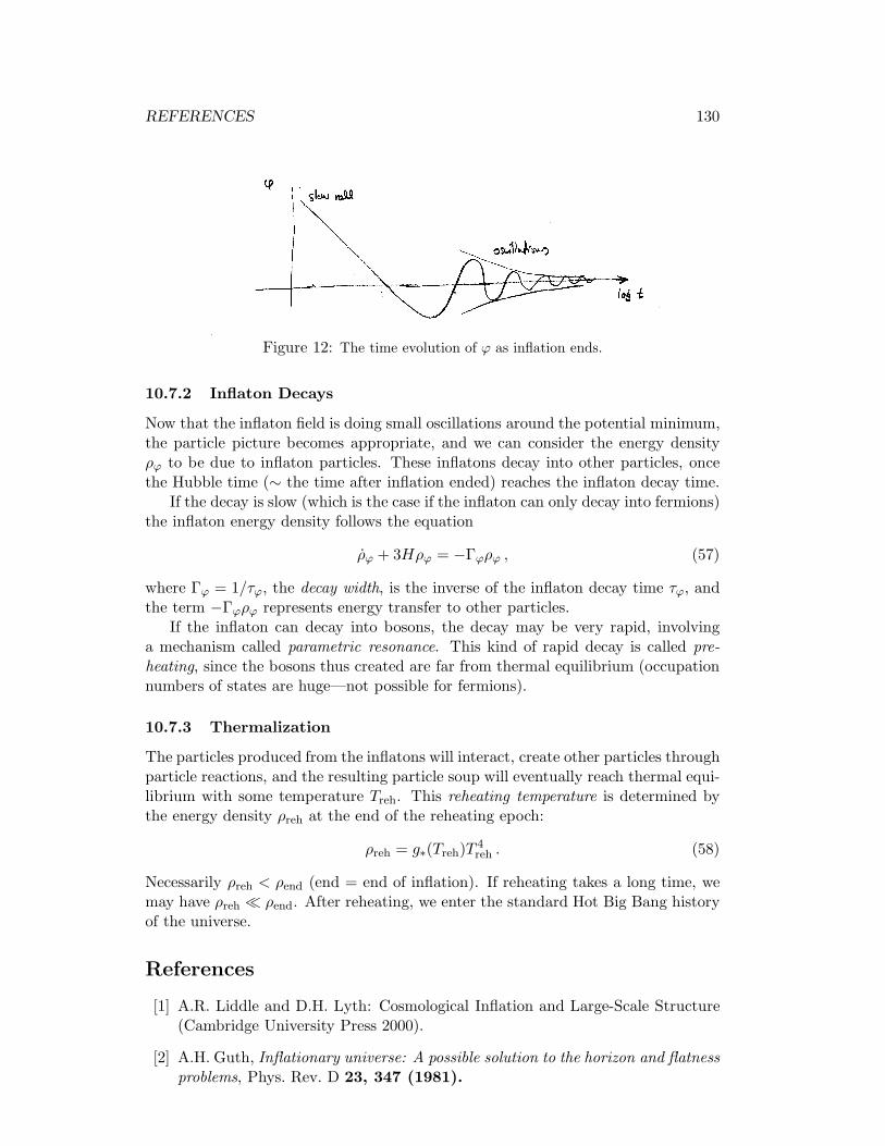
REFERENCES 130

Figure 12: The time evolution of ϕ as inflation ends.

10.7.2 Inflaton Decays

Now that the inflaton field is doing small oscillations around the potential minimum,the particle picture becomes appropriate, and we can consider the energy densityρϕ to be due to inflaton particles. These inflatons decay into other particles, oncethe Hubble time (∼ the time after inflation ended) reaches the inflaton decay time.

If the decay is slow (which is the case if the inflaton can only decay into fermions)the inflaton energy density follows the equation

ρϕ + 3Hρϕ = −Γϕρϕ , (57)

where Γϕ = 1/τϕ, the decay width, is the inverse of the inflaton decay time τϕ, andthe term −Γϕρϕ represents energy transfer to other particles.

If the inflaton can decay into bosons, the decay may be very rapid, involvinga mechanism called parametric resonance. This kind of rapid decay is called pre-heating, since the bosons thus created are far from thermal equilibrium (occupationnumbers of states are huge—not possible for fermions).

10.7.3 Thermalization

The particles produced from the inflatons will interact, create other particles throughparticle reactions, and the resulting particle soup will eventually reach thermal equi-librium with some temperature Treh. This reheating temperature is determined bythe energy density ρreh at the end of the reheating epoch:

ρreh = g∗(Treh)T 4reh . (58)

Necessarily ρreh < ρend (end = end of inflation). If reheating takes a long time, wemay have ρreh ≪ ρend. After reheating, we enter the standard Hot Big Bang historyof the universe.

References

[1] A.R. Liddle and D.H. Lyth: Cosmological Inflation and Large-Scale Structure(Cambridge University Press 2000).

[2] A.H. Guth, Inflationary universe: A possible solution to the horizon and flatnessproblems, Phys. Rev. D 23, 347 (1981).