10-1 Purchasing and Supply Scheduling Decisions Chapter 10 CR (2004) Prentice Hall, Inc. Press On Nothing in the world can take the place of persistence

10-1

Purchasing and Supply Scheduling Decisions

Chapter 10CR (2004) Prentice Hall, Inc.

Press On Nothing in the world can take the place of persistence. Talent will not. Nothing is more common than unsuccessful men with talent. Genius will not. Unrewarded genius is almost a proverb. Education will not. The world is full of educated derelicts. Persistence and determination alone are omnipotent.

10-2CR (2004) Prentice Hall, Inc.

Purchasing in Inventory Strategy

PL

AN

NIN

G

OR

GA

NIZ

ING

CO

NT

RO

LL

ING

Transport Strategy• Transport fundamentals• Transport decisions

Customer service goals

• The product• Logistics service• Ord. proc. & info. sys.

Inventory Strategy• Forecasting• Inventory decisions• Purchasing and supply

scheduling decisions• Storage fundamentals• Storage decisions

Location Strategy• Location decisions• The network planning process

PL

AN

NIN

G

OR

GA

NIZ

ING

CO

NT

RO

LL

ING

Transport Strategy• Transport fundamentals• Transport decisions

Customer service goals

• The product• Logistics service• Ord. proc. & info. sys.

Inventory Strategy• Forecasting• Inventory decisions• Purchasing and supply

scheduling decisions• Storage fundamentals• Storage decisions

Location Strategy• Location decisions• The network planning process

CR (2004) Prentice Hall, Inc.

A Typical Scheduling Diagram

ForecastForecast OrdersOrdersBuild schedule

Build schedule

InventoryInventory ShortagesShortages

Purchase order

releases

Purchase order

releases

To vendorsTo vendorsProduction release

Bill of materials

Bill of materials

The point: Supply is to inventory or to requirements

10-3


Supply to RequirementsMethods of scheduling

•Just-in-time concept

•Requirements planning

•KANBAN

Just-in-time

A philosophy of scheduling where the entire supply channel is synchronized to respond, in as short a time as possible, to the requirements of operations.

A philosophy of scheduling where the entire supply channel is synchronized to respond, in as short a time as possible, to the requirements of operations.


Supply to RequirementsThe characteristics are:

•Close relationship with a few suppliers and transport carriers

•Information is shared between buyers and suppliers

•Frequent production/purchase and transport of goods in small quantities

•Minimum inventory levels

•Uncertainties are to be eliminated wherever possible throughout the supply channel

•Why requirements become lumpy for the materials manager

•Setting the master schedule

-through derived demand patterns and bill of materials explosion

-forecasting

-orders on hand

Supply to Requirements (Cont’d)Requirements planning

Definition A formal, mechanical method of scheduling whereby the timing of purchases or supplies is determined by offsetting the requirements in the master production schedule.

Definition A formal, mechanical method of scheduling whereby the timing of purchases or supplies is determined by offsetting the requirements in the master production schedule.

CR (2004) Prentice Hall, Inc. 10-6

Supply to Requirements (Cont’d)

Time

Time

Order point

Order point

Leve

lLe

vel

0

0

Production order release

Order placement

(a) Field inventory (Finished product in warehouse)

(b) Factory inventory (Finished product at plant)

Why

dem

and

beco

mes

lum

py




Time

Order point

Leve

l

0

Purchase order release

(c) Component inventory (Supply stocks at plant)



•The mechanics of lot-for-lot scheduling given certain requirements and lead times

•Determining lot sizes

-Trading purchase price for inventory carrying cost

•Handling uncertainties in the master schedule

-Minimum inventory levels

-Part-period cost balancing

•Handling lead time uncertainties

10-10

MRP SchedulingExample

The master schedule for a particular part over the next 8 weeks shows requirements of:

1 2 3 4 5 6 7 8150 500 350 300 1000 800 700 500

The average lead-time to receive these parts from a vendor is 2 weeks. A previous order for 800 units has been placed with the vendor and will arrive by week 2. An inventory of 200 units is currently on hand.

Lot-for-lot scheduling

Purchase orders are matched on a one-for-one basis with requirements.


MRP Example (Cont’d)

Week 1 2 3 4 5 6 7 8

Require-ments 150 500 350 300 1000 800 700 500

Scheduledreceipts 800 300 1000 800 700 500

Quantityon hand 200 50 350 0 0 0 0 0 0

Purchasereleases 300 1000 800 700 500

Lot-for-lot scheduling (Cont’d)



MRP Example (Cont’d)Purchase order minimums

Vendors can set order minimum quantities to avoid the high cost of handling small orders. This will usually force some inventory into the system.

Part period cost balancing

The economically best order quantities can be set by balancing the cost of processing an order with the cost of carrying the inventory associated with ordering more than what is immediately needed.

Suppose it costs $120 to process and deliver each order. Inventory carrying costs are 25% per year, or $0.07 per unit per week on parts valued at $15.

10-12

Order min. qty.


Week 1 2 3 4 5 6 7 8

Require-ments 150 500 350 300 1000 800 700 500


Quantityon hand 200 50 350 0 200 0 0 0 0


Order minimumsSuppose the vendor has an order minimum of 500 units.



Part-Period Example (Cont’d)

An order is to be released for a quantity to just meet requirements or for a quantity that will meet several weeks’ requirements. Find the average inventory costs for ordering 1 week’s requirements, 2 weeks’ requirements, etc. The order quantity is the one that best matches the order processing cost.

Method Find the average inventory in each week. Average inventory is beginning inventory ending inventory/2, where beginning inventory is scheduled receipts quantity on hand. Ending inventory is beginning inventory – requirements. Therefore,


Part-Period Example (Cont’d)

Since the carrying cost of Q = 1,300 best matches the process/order cost of $120, then it is best to order 2 weeks ahead. After 2 weeks, compute for a new quantity.

50.255$2

08002

80018002

1800210007.0

6 & 4,5, Weeks )8001000300(

20.115$2

010002

1000130007.0

5 & 4 Weeks )1000300(

50.10$2

03000.07

4 Week )300(

CC

Q

CC

Q

CC

Q

Closestto $120process

cost

10-15

MRP Example (Cont’d)Safety stockUncertainties in the master schedule and in the lead times are sometimes handled by requiring a minimum quantity on hand to be maintained. Suppose a safety stock of 100 units is to be maintained with a 500-unit order-size minimum.

Week 1 2 3 4 5 6 7 8

Require-ments 150 500 350 300 1000 800 700 500


Quantityon hand 200 50 350 500 200 100 100 100 100


10-16


MRP Example (Cont’d)Setting the lead-time

Suppose there is a cost of delaying production when the parts do not arrive on time. A carrying cost of $5 per unit per day is incurred (cost is different from previous illustration for contrast). Lead-time averages 14 days (2 weeks) with a standard deviation of 3 days and is normally distributed. What is the proper lead-time to release orders?

We are looking for T* on the lead time distribution. First, we find the probability of delaying production from

cc

c

PC

PP

1



where

Pc = cost of having materials after they are needed ($/unit/day)

Cc = cost of having materials before they are needed ($/unit/day)

01.05005

5001

P

From a normal distribution table, this is a point of 2.33 standard deviations from the average lead time, or z = 2.33. Then,



)(*LT

szLTT

where

T* = order release time

LT = average lead-time

sLT = standard deviation of lead-time (days)

z = number of standard deviations between LT and T*

Hence, T* = 14 + 2.33(3) = 21 days

Lead-time should be considered 3 weeks instead of 2 weeks. This will force some inventory into the system.



P

LT=14

sLT=3

T*

Lead time distribution with order release point

10-21

Supply to Requirements (Cont’d)KANBAN

Definition A method of scheduling using the order point inventory control procedure, but with very low setup costs and very short lead-times.

Definition A method of scheduling using the order point inventory control procedure, but with very low setup costs and very short lead-times.

Characteristics of the scheduling method are:

•Models are repeated frequently in the master schedule. A typical master schedule for economies of scale might look like.

AAAAAABBBBBBAAAAAABBBBBB

but a KANBAN schedule would approach

ABABABABABABABABABABABABCR (2004) Prentice Hall, Inc.


Kanban (Cont’d)

•Lead-times are predictable because they are short and because suppliers are located near the site of operations

•Order quantities are small because setup or procurement costs are kept low

•Few vendors are used with high expectations of vendors and high level of cooperation with them

•Classic reorder point inventory control is used to determine reorder quantities and timing of purchases


KANBAN vs. Supply to Inventory

Factors KANBAN/JIT Scheduling Supply to InventoryInventory A liability. Every effort must

be expended to do away withit.

An asset. It protects against forecasterrors, machine problems, late vendordeliveries. More inventory is "safer."

Lot Sizes Size for immediate needs only.A minimum replenishmentquantity is desired for bothmanufactured and purchasedgoods.

Formulas are used. Optimum lotsizes frequently revised based on thetradeoff between the cost ofinventories and the cost of set up.

10-23


KANBAN vs. Supply to InventoryFactors KANBAN/JIT scheduling Supply to InventorySet Ups Make them insignificant. This

requires either extremely rapidchangeover to minimize theimpact on operations, or theavailability of extra machinesalready set up. Fast changeoverpermits small lot sizes to bepractical, and allows a widevariety of parts to be madefrequently.

Low priority. Maximum output is the usualgoal. Rarely does similar thought and effortgo into achieving quick changeover.

Queues Eliminate them. Whenproblems occur, identify thecauses and correct them. Thecorrection process is aidedwhen queues are small. If thequeues are small, it surfaces theneed to identify and fix thecause.

Necessary investment. Queues permitsucceeding operations to continue in theevent of a problem with the feedingoperation. Also, by providing a selection ofjobs, the factory management has a greateropportunity to match up varying operatorskills and machine capabilities, combine set-ups and thus contribute to the efficiency ofthe operation. 10-24



Factors KANBAN/JIT Scheduling Supply to InventoryVendors Co-workers. They're part of the team.

Multiple deliveries for all active itemsare expected daily. The vendor takescare of the needs of the customer, andthe customer treats the vendor as anextension of his factory.

Adversaries. Multiple sourcesare the rule, and it's typical toplay them against each other.

Quality Zero defects. If quality is not 100%,production is in jeopardy.

Tolerate some scrap. Scrap istracked and formulas aredeveloped for predicting it.

Equipmentmainten-ance

Constant and effective. Machinebreakdowns must be minimal.

As required. But not criticalbecause of queues available.

Lead times Keep them short. This simplifies thejob of marketing, purchasing, andmanufacturing as it reduces the needfor expediting.

The longer the better. Mostforemen and purchasing agentswant more lead time, not less.

10-25



Factors KANBAN/JIT Scheduling Supply to InventoryWorkers Management by consensus. Changes

are not made until consensus isreached, whether or not a bit of armtwisting is involved. The vitalingredient of "ownership" is achieved.

Management by edict. Newsystems are installed in spite ofthe workers. The concentrationis on measurements to determinewhether or not they're doing it.

10-26

Supply Chain Dynamics “Bullwhip Effect”

Time

Supply channel

Customer Customer

Firm A

Firm B

Firm C

Firm C

Firm AD

eman

d

Demand on upstream firms varies greatly with small changes in downstream demand



Bullwhip Effect (Cont’d)Reasons for the effectInternal•Demand shifts•Product/service

changes•Late deliveries•Incomplete shipments

External•Supply shortages•Engineering changes•New product/service

introductions•Product/service promotions•Information errors

Remedies•Centralize demand forecasting•Improve forecasting accuracy•Reduce lead-time uncertainties throughout the channel•Smooth response to change

10-28


Vendor Managed Inventory

•The supplier usually owns the inventory at the customer’s location

•The supplier manages the inventory by any means appropriate and plans shipment sizes and delivery frequency

•The buyer provides point of sale information to the supplier

•The buyer pays for the merchandise at the time of sale

•The buyer dictates the level of stock availability required

10-30

PurchasingWhat is purchasing?

•Primarily a buying activity

•A decision area to be integrated with overall materials management and logistics

•At times, an area to be used to the firm’s strategic advantage

Mission Securing the products, raw materials, and services needed by production, distribution, and service organizations at the right time, the right price, the right place, the right quality, and in the right quantity.

Mission Securing the products, raw materials, and services needed by production, distribution, and service organizations at the right time, the right price, the right place, the right quality, and in the right quantity.


10-31

Purchasing (Cont’d)

What is purchased?

•Price-Cost of goods-Terms of sale-Discounts

•Quality-Meeting specifications-Conformance to quality standards

•Service-On-time and damage-free delivery, order-filling accuracy, product availability

-Product supportCR (2004) Prentice Hall, Inc.

Purchasing (Cont’d)Importance of purchasing management

•Decisions impact on 40 to 60% of sales dollar•Decisions are highly leveraged

Activities of purchasing

•Selects and qualifies suppliers

•Rates supplier performance•Negotiates contracts•Compares price, quality, and service

•Sources goods•Times purchases

•Sets terms of sale•Evaluates the value received

•Measures inbound quality if not a responsibility of quality control

•Predicts price, service, and sometimes demand changes

•Specifies form in which goods are to be received


Importance of PurchasingLeverage principlecosts

CurrentSales+17%

Price+5%

Labor and

Salaries-50%

Overhead-20%

Purchases+8%

Sales $100 $117 $105 $100 $100 $100

Purchased goods and services

60 70 60 60 60 55

Labor and salaries

10 12 10 5 10 10

Overhead 25 25 25 25 25 25

Profit $5 $10 $10 $10 $10 $10

A company with $100 million in sales wishes to double profits. How to do it?

Conclusion Reducing purchase prices requires the least changeConclusion Reducing purchase prices requires the least change


Importance of PurchasingLeverage principlereturn on assets

Sales$10 million

Total costa

$9.5 million

Profit$500,000

Sales$10 million

Dividedby

Profitmargin

5%

Less

Sales$10 million

Returnon

assets10%

Investmentturnover2 timesTotal

assets$5 million

Dividedby

Inventoryc

$2 million

Multipliedby

(9.25 million)b

($750,000)

(7.5%)

(15.3%)

(2.04)

($4.9 million)($1.9 million)

aPurchases are 50% of total sales.bFigures in parentheses assume a 5% reduction in purchase prices.cInventory is 40% of total assets.

A 5% reduction in purchase price can lead to a 15% increase in return on assetsCR (2004) Prentice Hall, Inc.

10-34

10-35

Supplier SelectionCriteria for selecting suppliers

•Past or anticipated relations

-Honesty

-Financial viability

-Reciprocity

•Measured performance

-Price

-Responsiveness to change or requests

-On-time delivery

-Product or service backup

-Meeting quality goals


10-36

Supplier Selection (Cont’d)Single vendors

•Allows for economies of scale

•Consistent with the just-in-time philosophy

•Builds loyalty and trust

•May be only source for unique product or service

Multiple vendors

•Encourages price competition

•Diffuses risk

•May disturb supplier relations, reduce loyalty, reduce responsiveness, and cause variations in product

quality and serviceCR (2004) Prentice Hall, Inc.

10-37

Supplier Selection (Cont’d)Finding suppliers

•Personal contacts

•Trade publications

•Web sites, catalogs, and directories

•Advertisements and solicitations

Qualifying suppliers

•Previous experiences and formal rating schemes

•Word of mouth

•Samples of product

•Reputation

•Site visits and demonstrationsCR (2004) Prentice Hall, Inc.

10-38

Supplier Selection (Cont’d)

Criteria for selecting suppliers (Cont’d)

•Operational compatibility

-Informational compatibility

-Physical compatibility

•Ethical and moral issues

-Minority vendors

-Lowest price bidding

-Patriotic purchasing

-Open bidding but a pre-selected vendor



Supplier RatingExample of weighted checklist method for supplier evaluation

Scoring actual performance

Compare to best score of 100 and to scores for other suppliers.

Weight Factor Formula50% Quality 100% - % rejects25% Service 100% - 7% for each failure25% Price Lowest price offered

Price actually paid

Factor Weight Performance EvaluationQuality 50 5% rejects 50x(1-.05) = 47.50Service 25 3 failures 25x[1-(.07x3)] = 19.75Price 25 $100 25x($90/$100) = 22.50

Overall 89.75

10-39

Allocation to SuppliersAllocation methods

•Company policy considering risk, fairness, ethics, etc.

•Definitive methods

Example of a definitive methodThe Acme Company has received quotes for a component (X-16) that is part of a larger assembly (industrial motors). The prices are as follows:

SupplierShippinglocation FOB price

Philadelphia Tool Philadelphia $100 eaHouston Tool & Die Houston 101Chicago-Argo St Louis 99LA Tool Works Los Angeles 96

CR (2004) Prentice Hall, Inc.10-40


Allocation (Cont’d)The company has 3 plants to be supplied at Cleveland, Atlanta, Kansas City. The transportation rates, plant requirements (cwt.), and available supply limits (cwt.) are:

Shipping Kansas Avail-point Cleveland Atlanta City abilityPhiladelphia 2 3 5 5,000Houston 6 4 3 15,000St Louis 3 3 1 4,000Los Angeles 8 9 7 15,000Requirements 4,000 2,000 7,000

Each part weighs 100 lb. (1 cwt.) and rates are in $/cwt.

10-41


Allocation (Cont’d)

Purchase costs 13,000 x 96 = $1,248,000Transport to CLE 4,000 x 8 = 32,000Transport to ATL 2,000 x 9 = 18,000Transport to KC 7,000 x 7 = 49,000 Total $1,347,000

Current purchase: Buy from supplier with lowest price. Thus, all purchases from LA Tool for a total cost of:

Is buying based on lowest price a good strategy?

10-42

Allocation (Cont’d)Allocate using linear programming Purchase price

plus transport

Shipping Avail-point CLE ATL KC Dummy abilityPhila- 102 103 105 0delphia 4,000 1,000 5,000Houston 107 105 104 0

15,000 15,000Saint 102 102 100 0Louis 4,000 4,000 Los 104 105 103 0Angeles 1,000 3,000 11,000 15,000Require-ments 4,000 2,000 7,000 26,000


Allocation (Cont’d)Revised plan

PHI to CLE 102 x 4000 = $408,000PHI to ATL 103 x 1000 = 103,000STL to KC 100 x 4000 = 400,000LAX to ATL 103 x 1000 = 103,000LAX to KC 103 x 3000 = 309,000 Total $1,325,000

This allocation saves $22,000 per purchase

Now, asking “what if” questions can provide insight into good allocation plans.




What if CLE and KC markets are increased by 20% and ATL market is increased by 50%.

CLE ATL KCPHI 4800 200HOUSTL 2800 1200LAX 7200

Total cost = $1,657,400

Solution

Problem

10-45



What if Philadelphia price is increased by 10%?

Solution

CLE ATL KCPHIHOUSTL 2000 2000LAX 4000 5000

Total cost = $1,335,000

Problem

10-46



What if STL is no longer a supplier?

Solution

HOUSTLLAX 1000 7000

CLE ATL KCPHI 4000 1000

Total cost = $1,337,000

Problem

10-47



What if STL’s capacity is doubled?

Solution

CLE ATL KCPHI 4000 1000HOUSTL 1000 7000LAX

Total cost = $1,313,000

Problem

Observations Houston is a weak supplier. Perhaps some price concessions can be negotiated? Philadelphia is price sensitive and cannot withstand much of a price increase. St Louis is a valuable supplier and more capacity should be sought.

Observations Houston is a weak supplier. Perhaps some price concessions can be negotiated? Philadelphia is price sensitive and cannot withstand much of a price increase. St Louis is a valuable supplier and more capacity should be sought.

10-48

•Through just-in-time planning

-Material requirements planning for continuous work

-Gantt charts and CPM/PERT for project work

•Through inventory management

-Push methods

-Pull methods

•According to market conditions

-Speculative buying

-Forward buying

-Hand-to-mouth buying, or buying to current requirements

Timing of PurchasesMethods

10-49

Timing of Purchases (Cont’d)Speculative buying

Buying more than the foreseeable requirements at current prices in the hope of reselling later at higher prices. Some of the purchased quantities may be used in production and some simply resold. Generally a financial activity, not a materials management one.

Forward buyingBuying in quantities exceeding current requirements, but not beyond foreseeable needs. - Takes advantage of favorable prices in an unstable

market, or takes advantage of volume transportation rates

- Reduces risk of inadequate deliveryCR (2004) Prentice Hall, Inc. 10-50

Timing of Purchases (Cont’d)

Hand-to-mouth buying

Buying to satisfy immediate needs such as those generated through MRP. - Advantageous when prices are dropping - May improve cash flow by temporarily reducing

expenses of carrying inventory


Note: The reasonto look at

forecasting methods

Timing of Purchases (Cont’d)Forward buying example--volume buying

A firm is able to forecast the following price curve over the next two years with usage averaging 20,000 units per month

Objective To buy in larger volume when prices are rising and to buy only to immediate needs when prices are falling.

Objective To buy in larger volume when prices are rising and to buy only to immediate needs when prices are falling.


Timing of Purchases (Cont’d)Strategy Try purchasing every four months while prices are rising and hand-to-mouth purchasing when they are falling.

Strategy Try purchasing every four months while prices are rising and hand-to-mouth purchasing when they are falling.

Price upswing purchase cost

No of Cost TotalDate units per unit costJan 80,000 $2.00 $160,000May 80,000 2.35 188,000Sep 80,000 2.75 220,000_______ ________ 240,000 $568,000

Average cost per unit = 568,000/240,000 = $2.37 per unit


20,000 240,000 $593,800

Timing of Purchases (Cont’d)Price downswing purchase cost

Average cost per unit = 593,000/240,000 = $2.47 per unit

No of Cost TotalDate units per unit costJan 20,000 $2.86 $ 57,200Feb 20,000 2.83 56,600Mar 20,000 2.80 56,000Apr 20,000 2.75 55,000May 20,000 2.65 53,000Jun 20,000 2.55 51,000Jul 20,000 2.45 49,000Aug 20,000 2.35 47,000Sep 20,000 2.25 45,000Oct 20,000 2.15 43,000Nov 20,000 2.05 41,000

2.00 40,000Dec

Note: This is thesame average priceas hand-to-mouthbuying on price

upswing.



Timing of Purchases (Cont’d)Savings

Savings for one year out of two are:

%410047.2

37.247.2 reduction Price x

or $593,800 – 568,000 = $25,000

But trades with increased inventory

Buying in 80,000 lot quantities instead of 20,000 will add to inventory.

units 000,302

000,20000,80 This is the incremental

inventory neededfor forward buying

compared with H-to-M 10-55



Suppose inventory carrying costs are 25% per year on an approximate value of $2.37 per unit. Incremental inventory costs would be:

CC = 0.25(2.37)(30,000) = $17,775

Net savings = 25,000 – 17,775 = $7,225 in favor of forward buying. Now, try other lengths of forward buying, such as once a year, to see if further improvement can be made.


Timing of Purchases (Cont’d)Forward buying exampledollar averaging

Spend the same amount on each purchase with the idea of buying more when prices are low and less when they are high. This is a good strategy when prices are expected to rise over the long term and there is substantial uncertainty as to the actual price level. Because under-supply may occur, some level of inventory will need to be maintained.

Dollar averaging procedure

•Estimate the average price over the planning period•Estimate the average usage for each purchase period•Compute the dollars to be spent each time a

purchase is made

10-57



Assumption Adequate inventory is available to handle the needs of production.

Example Consider the first year of the data. The average price is about $2.50 per unit. Suppose purchases are to be made every 3 months at an average usage rate of 20,000 units per month. Hence, the dollar purchase should be 20,000 x 3 x 2.50 = $150,000.


Timing of Purchases (Cont’d)Results

No of Cost TotalDate units per unit costJan 75,000 2.00 $150,000Apr 66,667 2.25 150,000Jul 58,824 2.55 150,000Oct 53,571 2.80 150,000_______ _______ 254,062 600,000

Average price = 600,000/254,062 = $2.36

A purchase cost saving over hand-to-mouth buying of

[(2.47 – 2.36)/2.47] x 100 = 4.5%



And don’t forget the inventory effects!

The average purchase quantity is 254,062/4 = 63,516 so that the average inventory has increased from hand-to-mouth buying by:

units 575,212

000,20515,63

CC = 0.25(2.36)(21,575) = $12,729

So, the net savings are (2.47 – 2.36)x254,062 – 12,729 = $15,218 per year for this single item


Quantity Discounts

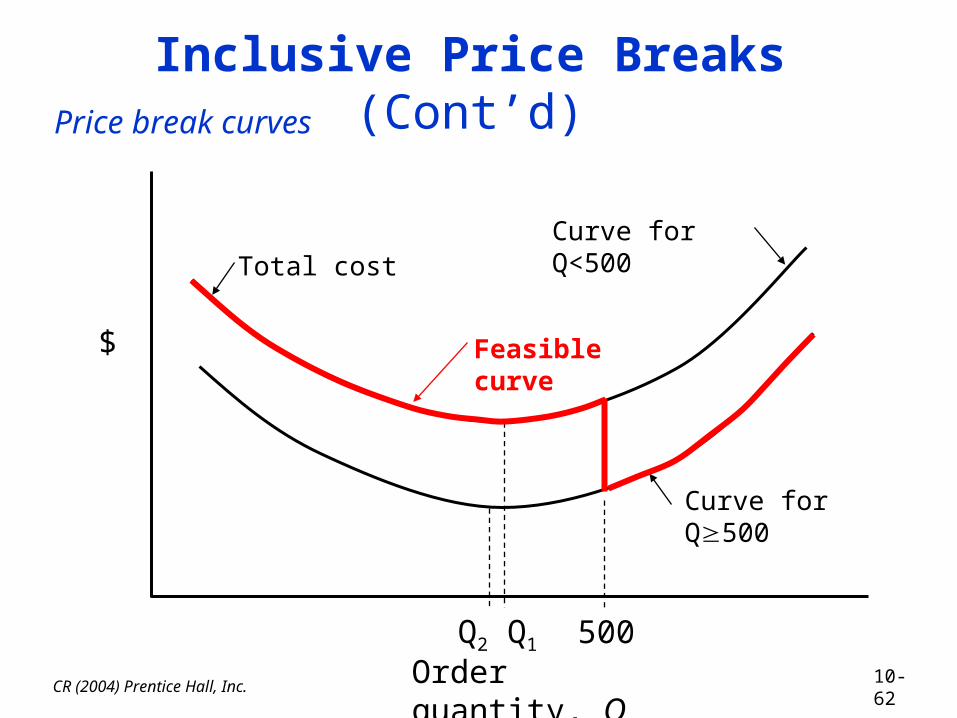
Inclusive price breaks

A simple, one price break can be expressed as

Quantity, Qi Price, Pi

0 < Qi < Q1 P1

Qi Q1 P2

Finding the price for minimum cost requires•Computing EOQ for each price, P that is feasible. Compute total cost for feasible Qs•Setting Q at minimum quantity in each price range and compute total cost•Selecting Q with minimum cost


Inclusive Price Breaks (Cont’d)Price break curves

$

500Order quantity, Q

Q2 Q1

Curve for Q<500Total cost

Curve for Q500

Feasible curve

10-62

Quantity Discounts

Example Suppose a 5% discount is given for all items when purchase quantities are greater than or equal to 500 units. Otherwise, we have:

d = 50 units/week I = 10%/year S = $10/order LT = 3 weeks C = $5/unit (< 500 units)

Because of discontinuities in the total cost curve, the correct order quantity is found by checking the points of discontinuity in the total cost curve as well as the Q values determined from the EOQ formula.



Inclusive Price Breaks (Cont’d)The relevant total cost equation is written to include the purchase price.

2i

ii

ii

QIC

QDSDpTC

The total cost for Q* determined for Q < 500 units. Q* = 322 from EOQ formula.

$13,1612

2)0.10(5)(32322

2,600(10)5(2,600) 1

TC

At the price break point (500 units).

$12,5212

5)5000.10(5)(.9500

2,600(10)00)5(.95)(2,6 2

TC

10-64


Inclusive Price Breaks (Cont’d)

Finally, check to see if Q* for the discounted price is feasible.

units 33195)(.10)(5)(.

0)2(2,600)(1 *Q

This value is infeasible since 331 units are based on an item value with the price discount and an order quantity of at least 500 units is required. Thus, the best order quantity for minimum cost is 500 units.


Example Suppose the previous 5% discount applies only to purchases > 500 units. That is, the first 500 units are priced at $5 per unit, but all units over 500 are priced at 0.95 x $5 = $4.75. Because of the declining average cost, the optimum Q* is found by trial and error. We can develop a table for the total cost equation. Q* is about 1,000 units.

Quantity Discounts (Cont’d)Noninclusive price breaks

Price discount only applies to the items beyond the price break quantity. Average price continues to drop with increasing purchase quantities.


Quantity Discounts (Cont’d)

Cost for

Cost for

Q1

0

To

tal c

ost

Purchase quantity, Qi

0 1 Q Qi

Q Qi 1

Price break curve-noninclusive discounts


Noninclusive Price Breaks (Cont’d)Q Average Unit Price PD DS/Q ICQ/2 Total cost, $

300 $5 $13,000 $86.67 $75.00 $13,162

400 5 13,000 65.00 100.00 13,165

500 5 13,000 52.00 125.00 13,177

600 5x500+100x4.75600

12,896 43.33 148.80 13,088

800 5x500+300x4.75800

12,756 32.50 196.25 12,985

900 5x500+400x4.75900

12,711 28.89 220.00 12,960

1,000 5x500+500x4.751000

12,675 26.00 243.75 12,945

1,500 5x500+1000x4.751500

12,567 17.33 362.50 12,947

2,000 5x500+1500x4.752000

12,513 13.00 481.25 13,007


Quantity Discounts (Cont’d)Deal buyingA one-time buying opportunity. Determining the quantity to purchase requires balancing the benefits of a price discount against extra inventory holding costs. The optimal purchase quantity is found from:

dppQ

IdpdD

Q

*

)(ˆ

where

units size, order special units discount, the before quantity order optimal

units demand, annual %/year cost, carrying annual

$/order cost, order $/unit discount, the before unit per price

$/unit decrease, price unit

QQDI

Spd

*


Quantity Discounts (Cont’d)Example An item has a delivered price of $72/unit. Annual purchases are for 4,000 units. Ordering costs are $50/order and carrying costs are 25%/year. A one-time $5/unit discount is offered. What should the order size be?

SolutionFind nondiscounted order quantity

units 149)72(25.0

)50)(000,4(22* ICDS

Q

And special order quantity

units 354,1)572()149(72

25.0)572()4000(5

)(ˆ

*

dp

pQIdp

dDQ

Documents

10-1 Purchasing and Supply Scheduling Decisions Chapter 10 CR (2004) Prentice Hall, Inc. Press On Nothing in the world can take the place of persistence