1

Topic 7

Part I Partial DifferentiationPart II Marginal Functions Part II Partial ElasticityPart III Total DifferentiationPart IV Returns to scale

Jacques (4th Edition): 5.1-5.3

2

Functions of Several Variables

More realistic in economics to assume an economic variable is a function of a number of different factors:

Y =f(X, Z)

Demand may depend on the price of the good and the income level of the consumer

Qd =f(P,Y)

Output of a firm depends on inputs into the production process like capital and labour

Q =f(K,L)

3

Graphically

Sketching functions of two variables Y= f (X, Z)

Sketch this function in 3-dimensional space

or plot relationship between 2 variables for

constant values of the third

4

For example I

Consider a linear function form:

y =a+bx+cz

For different values of z we can represent the relationship between x and y

Y

X

Y=a+bX+cZ

a +cZ0 ++a

Y

X

a+cz0

a+cz1

z1

z0

x0 x1

5

For example II

Consider a non-linear function form: Y=XZ

0<< 1 & 0<< 1 For different values of

z we can represent the relationship between x and y

X

Y

z =1

z >1

x0 x1

6

Part I: Partial Differentiation (Differentiating functions of several variables)

Recall, function of one variable y = f(x):

One first order derivative: )x('fdx

dy

One Second order derivative: )x(''fdx

yd

2

2

7

Consider our function of two variables:

Y= f (x, z) = a + bx + cz

TWO First Order Partial Derivatives

bffx

yx

1 Differentiate with respect to x, holding z constant

cffz

yz

2 Differentiate with respect to z, holding x constant

8

FOUR Second Order Partial DerivativesSecond Own and Cross Partial Derivatives

0112

2

ff

x

yxx

0222

2

ff

z

yzz

012

2

ffzx

yxz

021

2

ffxz

yzx

9

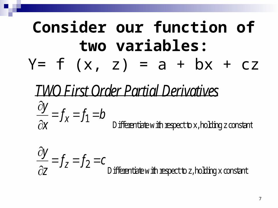
Consider our function of two variables: Y= f (X, Z) = XZ

First Partial Derivatives

Y/X = fX = X-1Z > 0

Y/Z = fZ = XZ-1 > 0

10

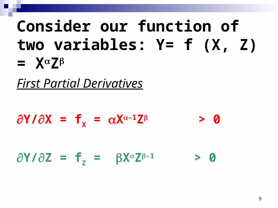
Since Y/X = fX = X-1Z

Y/Z = fZ = XZ-1

Second own partial

2Y/X2 = fXX = (-1)X-2Z < 0

2Y/Z2 = fZZ = (-1) XZ-2 < 0

Second cross partial

2Y/XZ = fXZ = X-1Z-1 > 0

2Y/ZX = fZX = X-1Z-1 > 0

11

Example Jacques Y= f (X, Z) = X2 +Z3

fX = 2X > 0 Positive relation between x and y

fXX = 2 > 0 but at an increasing rate with x

fXZ = 0, (= fzx) and a constant rate with z

impact of change in x on y is bigger at bigger values of x but the same for all values of z

fZ = 3Z2 > 0 Positive relation between z and y

fZZ = 6Z > 0 but at an increasing rate with z

fZX = 0 (= fxz) and a constant rate with x

impact of change in z on y is bigger at bigger values of z, but the same for all values of x

12

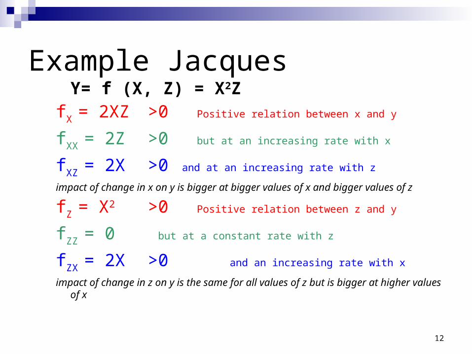
Example Jacques Y= f (X, Z) = X2Z

fX = 2XZ >0 Positive relation between x and y

fXX = 2Z >0 but at an increasing rate with x

fXZ = 2X >0 and at an increasing rate with z

impact of change in x on y is bigger at bigger values of x and bigger values of z

fZ = X2 >0 Positive relation between z and y

fZZ = 0 but at a constant rate with z

fZX = 2X >0 and an increasing rate with x

impact of change in z on y is the same for all values of z but is bigger at higher values of x

13

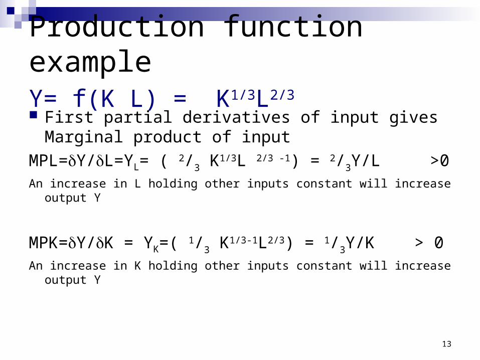
Production function exampleY= f(K L) = K1/3L2/3 First partial derivatives of input gives Marginal

product of input

MPL=Y/L=YL= ( 2/3 K1/3L 2/3 -1) = 2/3Y/L >0

An increase in L holding other inputs constant will increase output Y

MPK=Y/K = YK=( 1/3 K1/3-1L2/3) = 1/3Y/K > 0

An increase in K holding other inputs constant will increase output Y

14

MPL = Y/L = ( 2/3 K1/3L -1/3) = 2/3Y/L .

MPK = Y/K = ( 1/3 K-2/3L2/3) = 1/3Y/K .

Second Own derivatives of input gives Marginal Returns of input (or the change in the marginal product of an input with the level of that input)

Y/L2 = -2/9 K1/3L -4/3 < 0 Diminishing marginal returns to L (the change in MPL

with L shows that the MPL decreases at higher values of L)

Y/L2 = -2/9 K-5/3L2/3 < 0 Diminishing marginal returns to K (the change in the MPK

with K shows that the MPK decreases at higher values of K)

15

Part II: Partial Elasticity e . g c o b b - d o u g l a s p r o d u c t i o n f u n c t i o n Y = f ( K L ) = A K

L

E l a s t i c i t y o f O u t p u t w i t h r e s p e c t t o L

Y L = Y

L

L

Y

LL

YY

/

/

= ( A K

L - 1 ) . L / Y

= Y / L . L / Y = E l a s t i c i t y o f O u t p u t w i t h r e s p e c t t o K

Y K = Y

K

K

Y

KK

YY

/

/

= ( A K - 1 L

) . K / Y

= Y / K . K / Y =

16

Elasticity of Output with respect to L

YL = Y

L

L

Y

= ( 2/3 K1/3L 2/3 -1). L/Y = 2/3Y/L . L/Y = 2/3

Elasticity of Output with respect to K

YK = Y

K

K

Y

= ( 1/3 K 1/3 -1L 2/3). K/Y = 1/3Y/K . K/Y = 1/3

e.g. Y= f(K L) = K1/3L2/3

17

Q = f(P,PS,Y) = 100-2P+PS+0.1Y

P = 10, PS = 12, Y= 1000 Q=192 

Partial Own-Price Elasticity of Demand

QP = Q/P. P/Q =

-2 * (10/192) = - 0.10

Partial Cross-Price Elasticity of Demand

QPS = Q/PS. PS/Q =

+1 * (12/192) = 0.06

Partial Income Elasticity of Demand

QI = Q/Y. Y/Q =

+0.1 * (1000/192) = 0.52

e.g. demand function Q = f( P, PS, Y)

18

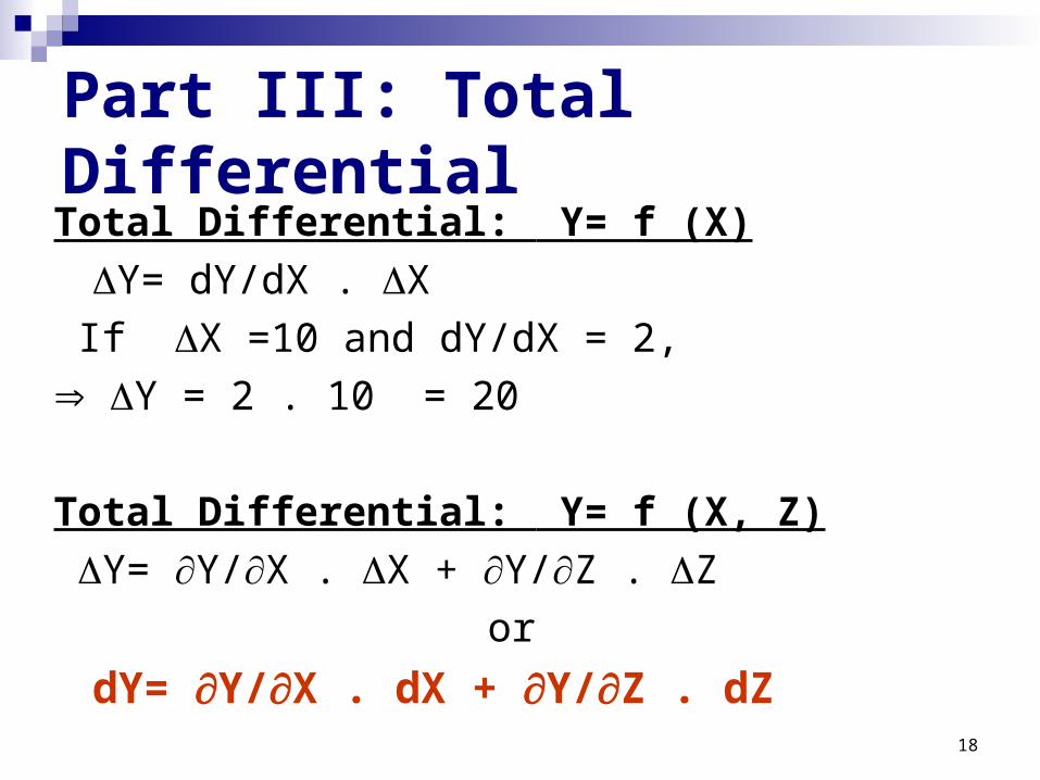
Part III: Total Differential Total Differential: Y= f (X)

  Y= dY/dX . X

 If X =10 and dY/dX = 2,

Y = 2 . 10 = 20

 

Total Differential: Y= f (X, Z)

 Y= Y/X . X + Y/Z . Z

or

dY= Y/X . dX + Y/Z . dZ

19

Example: Y= f (K, L) = Y = K1/3L2/3

 dY= Y/K . dK + Y/L . dL

or

dY= (1/3 K-2/3L2/3).dK + (2/3 K

1/3L-1/3).dL

Rewriting:

dY= (1/3 K1/3K-1L2/3).dK + (2/3 K

1/3L2/3L-1).dL

or

dY= 1/3.Y/K . dK + 2/3.

Y/L. dL

To find proportionate change in YdY/Y= 1/3.

dK/K + 2/3. dL/L

20

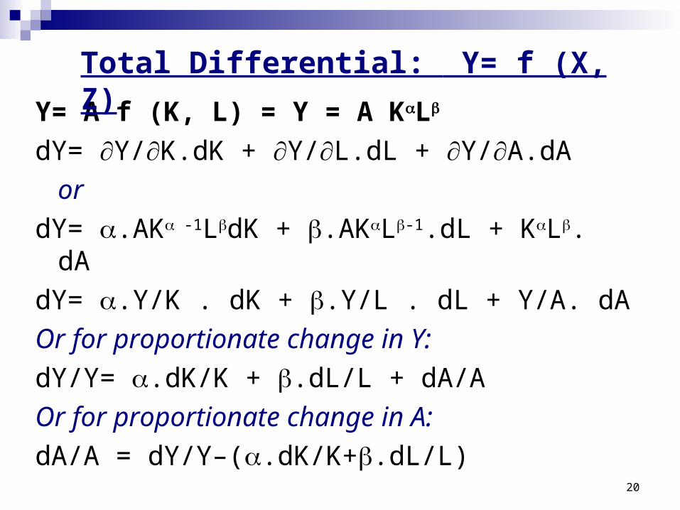
Y= A f (K, L) = Y = A KL

dY= Y/K.dK + Y/L.dL + Y/A.dA

or

dY= .AK -1LdK + .AKL-1.dL + KL. dA

dY= .Y/K . dK + .Y/L . dL + Y/A. dA

Or for proportionate change in Y:

dY/Y= .dK/K + .dL/L + dA/A

Or for proportionate change in A:

dA/A = dY/Y–(.dK/K+.dL/L)

Total Differential: Y= f (X, Z)

21

Part IV: Returns to Scale Returns to scale shows the change in Y due to a proportionate

change in ALL factors of production . So if Y= f(K, L)

Constant Returns to Scale

f(K, L ) = f(K, L) = Y

Increasing Returns to Scale

f(K, L ) > f(K, L) > Y

Decreasing Returns to Scale

f( K, L ) < f(K, L) < Y 

22

Cobb-Douglas Production Function: Y = AKL

 

Quick way to check returns to scale in Cobb-Douglas production function

Y = AKL then if + = 1 : CRS

if + > 1 : IRS

if + < 1 : DRS

23

 

Y*= f(K, L) = A (K)( L)

Y*= A K L = + AKL = + Y

+ = 1 Constant Returns to Scale  

+ > 1 Increasing Returns to Scale  

+ < 1 Decreasing Returns to Scale

Example: Y= f(K, L) = A KL

24

Homogeneous of Degree r if: f(X, Z ) = r f(X, Z) = r Y

Homogenous function if by scaling all variables by , can write Y in terms of r

Note superscripts!

Note then, for cobb-douglas Y = KL, the function is homogenous of

degree +

25

X fX + Z fZ = r f(X, Z) = rY 

E.g. r =1, Constant Returns to Scale  

If Y= f(K, L) = A KL(1-)

Does K fK + L fL = rY = Y ?

 

K (Y/K) + L((1-)Y/L) = ?

Y + (1-)Y = Y + Y -Y = Y

Thus, Eulers theorem shows

(MPk * K ) + (MPL * L) = Y in the case of homogenous production functions of degree 1

Eulers Theorem

26

then Y(K, L) = (K)½ (L)½

= ½K½ ½L½

= 1 K½ L½

= Y

homogenous degree 1..... constant returns to scale 

Eulers Theorem: show that

K.Y/K + L.Y/L = r.Y = Y (r=1 as homog. degree 1)

 = K. (½.K½ -1.L½) + L.(½.K½.L½ -1)

= K(½. Y/K) + L(½.Y/L)

= ½.Y + ½.Y = Y

Example .. If Y = K½ L½

27

Summary: Function of Two Variables Partial Differentiation -

Production Functions– first derivatives (marginal product of K or L) and second derivatives (returns to K or L)

Partial Elasticity – Demand with respect to own price, price of another good, or income

Total Differentials Returns to ScalePlenty of Self-Assessment Problems and

Tutorial Questions on these things….