Embed Size (px)
Citation preview

1 The Ising model
This model was suggested to Ising by his thesis adviser, Lenz. Isingsolved the one-dimensional model, ..., and on the basis of the factthat the one-dimensional model had no phase transition, he assertedthat there was no phase transition in any dimension. As we shallsee, this is false. It is ironic that on the basis of an elementarycalculation and erroneous conclusion, Ising’s name has become amongthe most commonly mentioned in the theoretical physics literature.But history has had its revenge. Ising’s name, which is correctlypronounced “E-zing,” is almost universally mispronounced “I-zing.”
Barry Simon
1.1 Definitions
The Ising model is easy to define, but its behavior is wonderfully rich. Tobegin with we need a lattice. For example we could take Zd, the set of pointsin Rd all of whose coordinates are integers. In two dimensions this is usuallycalled the square lattice, in three the cubic lattice and in one dimension itis often refered to as a chain. (There are lots of other interesting lattices.For example, in two dimensions one can consider the triangular lattice or thehexagonal lattice.) I will use letters like i to denote a site in the lattice. Foreach site i we have a variable σi which only takes on the values +1 and −1.Ultimately we want to work with the full infinite lattice. One approach todoing this is to first work with finite lattices and then try to take an “infinitevolume limit” in which the finite lattice approaches the full infinite lattice insome sense. (A different approach will be described latter.) In the case ofthe lattice Zd we could start with the subset
ΛL = {(i1, i2, · · · , id) : |ij | ≤ L, j = 1, 2, · · · , d}
and then let L → ∞.The subset ΛL is finite, so the number of possible spin configurations
{σi}i∈ΛLis finite. We will use σ as shorthand for one of these spins configu-
rations, i.e., an assignment of +1 or −1 to each site. We are going to definea probability measure µL on this set of configurations. It will depend on an
1
“energy function” or “Hamiltonian” H . The simplest choice for H is
H(σ) = −∑
i,j∈ΛL:|i−j|=1
σiσj
The sum is over all pairs of sites in our finite volume which are nearestneighbors in the sense that the Euclidean distance between them is 1. Theprobability measure is given by
µL(σ) = exp(−βH(σ))/Z
where Z is a constant chosen to make this a probability measure. Explicitly,
Z =∑
σ
exp(−βH(σ))
where the sum is over all the spin configurations on our finite volume. In ourdefinition of H we have only included the nearest neighbor pairs such thatboth sites are in the finite volume. This is usually called “free” boundaryconditions.
The possibility of imposing other boundary conditions will be importantin the discussion of phase transitions. We could add to the Hamiltoniannearest neighbor pairs of sites with one site in ΛL and the other site outsideof Λ. We then specify some fixed choice for each spin just outside of Λ. Forexample we might take all these outside spins to be +1. We will refer tothis as + boundary conditions. − boundary conditions are defined in theobvious way. Boundary conditions that use a mixture of + and − for thefixed boundary spins are of interest, e.g., in the study of domain walls orinterfaces. We will encounter them later.
Having defined a probability measure we can compute expectations withrespect to it. Of course, since the probability space is finite these expectationsare nothing more than finite sums. Physicists denote this expectation or sumby < >. For example,
< σ0 >=1
Z
∑
σ
σ0 exp(−βH(σ))
gives the average value of the spin at the origin. When we need to makeexplicit which boundary conditions we are using we will write < >+, <>− or < >free. If we use free boundary conditions then the model has
2

what is called a “global spin flip” symmetry. This simply means that ifwe replace every spins σi by −σi, then H(σ) does not change. Since σ0
changes sign under this transformation, we see that < σ0 >free= 0. Thisargument does not apply in the case of + or − boundary conditions. Avery important question is how much < σ0 > depends on the choice of theboundary conditions. We will address this question in the next section.
There is nothing special about the spin at the origin. We can computethe expectation of any function that only depends on the spins in the volumeΛ. Two that are of particular interest in physics are the magnetization
M =<∑
i∈Λ
σi >
and the energyE =< H >
Both of these quantities will grow like |Λ| as the volume goes to infinity. Toobtain something which has a chance of having an infinite volume limit weneed to divide them by the number of sites in the volume. The result ofdoing this for the energy is usually called the energy per site. For the totalmagnetization the result is often called simply the magnetization.
As we said at the start we eventually want to look at the infinite lattice.So we would like to take the limit as L → ∞ of quantities like the magneti-zation, expectations like < σ0 >L or more generally expectations < f(σ) >L
where f(σ) is any function that only depends on finitely many spins. Thisinfinite volume limit is often called the “thermodynamic” limit. The questionof its existence is a monumental one, but we will not have anything to sayabout it. However, we do want to introduce a slightly more mathematicalpoint of view of the infinite volume limit which we will pursue further insection 1.4. The reason for the restriction to finite volumes was to have onlya finite number of terms in the Hamiltonian. The infinite volume Hamilto-nian is only a formal creature, although it is often written down with theunderstanding that some sort of limiting process is needed. However, it doesmake sense to talk about probability measures on the infinite lattice. Thespace of configurations on the lattice Zd is {−1, +1}Zd
and this space has anatural topology - the product topology that comes from using the discretetopology on {−1, +1}. Hence the Borel sets provide a σ-algebra and we cantalk about Borel probability measures on the space of spin configurations.What one would like to show is that µ+
L converges to such a measure µ+ in
3
the sense that
limL→∞
< f(σ) >+
L=
∫
f(σ)dµ+
for functions f(σ) which only depend on finitely many spins. Integrals withrespect to such an infinite volume limit are often denoted < >, and wewill follow this convention. In this case it is natural to denote it by < >+
to indicate the possible dependence on the + boundary conditions used todefine the finite volume measure.
corr
elat
ion
leng
th
beta
Figure 1: Qualitative behavior of the correlation length as a function ofinverse temperature
Another quantity of physical interest which will play a major role in therenormalization group is the correlation length. A natural question is howmuch the spins σi and σj at two sites are correlated, especially if the spinsare far apart. The simplest measurement of this is
< σiσj > − < σi >< σj >
If the spins are independent then this quantity would be zero. This quantityis called a “truncated” correlation function and denoted by < σi; σj >. Whattypically happens is that this quantity decays exponentially as |i − j| → ∞for all values of β but one. So
< σi; σj >∼ exp(−|i − j|/ξ)
4
as |i − j| → ∞ where ξ is a length scale which is called the “correlationlength”. The behavior of this correlation length as a function of β is typicallythat shown in figure ??. The correlation length is to some extent a measure ofhow interesting the system is. A short correlation length means that distantspins are very weakly correlated.
We end this section by defining a few other quantities of physical interest.Before we do this we first introduce a slightly more general Hamiltonian. Ifthere is an external magnetic field on the system then the energy is given by
H = −∑
<i,j>
σiσj − h∑
i
σi
where h, the magnetic field is an external parameter. Of course for this tomake sense we must restrict to a finite volume and specify how we treat theboundary. The “free energy” F is defined by
exp(−βF ) = Z =∑
σ
exp(−βH)
F will be a function of the two parameters β and h and the choice of thefinite volume. It will usually grow with the number of sites in the volume.The free energy per site, f , is simply F divided by the number of sites. Itought to have an infinite volume limit. If we differentiate the free energy persite with respect to the magnetic field we get minus the magnetization,
m = −∂f
∂h
When we defined the magnetization before there was no magnetic field termin H . To obtain this magnetization we should set h = 0 after taking thederivative. However, we can talk about the magnetization of the systemwith an external field present, h 6= 0. The magnetization is then a functionof β and h. The derivative of the magnetization with respect to h is calledthe magnetic susceptibility and denoted by χ,
χ =∂m
∂h= −∂2f
∂h2
By taking the derivative of βf with respect to β one obtains the energy persite. The second derivative of f with respect to β is known as the specificheat and denoted
C =∂2f
∂β2
5
In the above definitions we would like to work with the infinite volumelimit of the free energy per site f . This limit is known to exist under verygeneral conditions. However, there is no reason that all the derivatives wehave been happily writing down need exist. At some values of the parametersthey will not, and this lack of analyticity is another way of detecting phasetrasitions.
Exercises:
1.1.1 (easy) By explicity computing ∂2f∂h2 , show that the susceptibility can be
written as a sum of truncated correlation functions:
χ = β∑
i,j∈Λ
< σi; σj >
1.1.2 (long, but important) The partition function for the Ising chain −L,−L+1, · · · , L − 1, L with various boundary conditions is
Zfree =∑
σ−L,···,σL
exp(βL−1∑
i=−L
σiσi+1)
Z+ =∑
σ−L,···,σL
exp(β
L−1∑
i=−L
σiσi+1 + βσ−L + βσL)
Z− =∑
σ−L,···,σL
exp(β
L−1∑
i=−L
σiσi+1 − βσ−L − βσL)
Zfree is easy to compute. Note that
∑
σL
exp(βσL−1σL) = 2 cosh(β)
regardless of what the value of σL−1 is. Use this to show that Zfree =[2 cosh(β)]2L+1.
To compute correlation functions it is useful to introduce something calledthe transfer matrix. Let T be the two by two matrix
T =
(
eβ e−β
e−β eβ
)
6
Normally one would write the entries of such a matrix as Tij with i, j runningfrom 1 to 2. Here we will denote the entries by T (σ, σ′) where σ and σ′
take on the values +1 and −1 in that order. So T (+1, +1) is the upperleft entry of the matrix. The important thing to note is that we now haveT (σi, σi+1) = exp(βσiσi+1). Define a vector
φ+ =
(
eβ
e−β
)
Show thatZ± = (φ±, T 2Lφ±)
Compute the eigenvalues and eigenvectors of T . Use this to show
Z+ = Z− = [2 cosh(β)]2L+2 + [2 sinh(β)]2L+2
Show that the free energy per site has an infinite volume limit and it is thesame for all three choices of boundary conditions.
Let D be the matrix
D =
(
1 00 −1
)
Show that
< σ0 >+=(φ+, TLDTLφ+)
(φ+, T 2Lφ+)
Use this and your diagonalization of T to show that < σ0 >+→ 0 as L → ∞.Show that
< σ0σl >+=(φ+, TLDT lDTL−lφ+)
(φ+, T 2Lφ+)
Use this to show that the infinite length limit of this correlation functionexists and is given by
limL→∞
< σ0σl >+= (tanh(β))l
and so the correlation length is given by
ξ =−1
log(tanh(β))
Sketch a graph of this correlation length as a function of β.
7

1.2 Phase transitions - the role of the boundary conditions
There are a variety of ways to look at phase transitions. We will startby asking whether or not the boundary conditions make a difference in theinfinite volume limit. Let’s start with a very specific instance of this question.In a finite volume we might guess that + boundary conditions would makethe spin at the origin a little more likely to be +1 than −1. This is indeedthe case; in fact we will prove that < σ0 >+
L> 0 in a moment. The importantquestion is what happens when we take the infinite volume limit, L → ∞.Does < σ0 >+
L converge to zero or to some nonzero value? (There is of coursethe third possibility that it does not coverge at all.) The answer depends onthe parameter β.
Theorem 1.2.1: If the number of dimensions is at least two, then there isa positive number βc such that for β < βc the limit limL→∞ < σ0 >+
L existsand is zero while for β > βc the limit exists and is strictly greater than zero.
We will only prove a weaker (but still very interesting) version of thistheorem. What we will show is that there are two positive constants β1 andβ2 such that if β < β1 then the limit is zero, while if β > β2 the limit isnot zero. β1 will be much smaller than β2, so our proofs won’t say anythingabout what happens in the rather large interval [β1, β2].
We start with the case of small β. This is the same as the temperaturebeing large, and this regime is usually called the “high temperature” regime.Of course if β = 0 then the spins are independent and the model is completelytrivial. The intuition is that if β is small, then the spins should only be weaklycorrelated. The influence of the boundary condition will decay rapidly as wemove in from the boundary.
When β is small, a natural approach is to attempt an expansion aroundthe trivial case of β = 0. This can be done, but it is not a trivial affair. Someexplanation of why it is not trivial will help to motivate the following proof.Consider the average value of the spin at the origin:
< σ0 >=
∑
σ σ0 exp(−βH(σ))∑
σ exp(−βH(σ))
For a finite volume the numerator and denominator are obviously entirefunctions of β. To conclude that their quotient is analytic somewhere weneed to know that the denominator does not vanish there. At β = 0 thedenominator is not zero, and so it does not vanish in a neighborhood of
8

zero. However, the region in which it does not vanish will depend on thefinite volume we are considering and may well shrink to just the origin as wetake the infinite volume limit. Note that if we expand either the numeratoror denominator in a power series about β = 0, the coeffecients will have astrong volume dependence. (The coeffecient of βn will grow like the numberof sites raised to the n.) By contrast we would hope that < σ0 > is analyticin a neighborhood of β = 0 with coeffecients that actually have a limit in theinfinite volume limit. (This is true although we will not prove it.) The crucialobservation is that there must be a lot of cancellation going on betweenthe numerator and denominator. This need to “cancel the numerator anddenominator” will appear in our proofs.
Theorem 1.2.2: In any number of dimensions there is a positive numberβ1 such that for β < β1 the limits limL→∞ < σ0 >+
L and limL→∞ < σ0 >−L
are both zero. (β1 will depend on the number of dimensions.)
Proof: The quantity σiσj only takes on the values +1 and −1. This and thefact that sinh and cosh are odd and even functions respectively, yields thefollowing identity.
exp(βσiσj) = cosh(σiσjβ) + sinh(σiσjβ)
= cosh β + σiσj sinh β = cosh β[1 + σiσj tanh β]
Using this identity we can rewrite the partition function as
Z =∑
σ
exp(∑
<i,j>
σiσj) = (cosh β)N∑
σ
∏
<i,j>
[1 + σiσj tanh β]
N is the number of bonds in the sum in the original Hamiltonian. We nowexpand out the product over the N bonds < i, j >. A term in the resultingmess is specified by choosing either 1 or σiσj tanh β for each bond < i, j >.Some of the bonds < i, j > have one site outside the volume. For these bondsσi is fixed to be +1 for the site outside the volume and σi is not summedover in the sum on σ. We let B denote the set of bonds for which we takeσiσj tanh β. Then
Z = (cosh β)N∑
σ
∑
B
∏
<i,j>∈B
σiσj tanhβ
where B is summed over all subsets of the set of nearest neighbor bonds suchthat at least one of the endpoints is in the finite volume. Letting |B| denote
9
the number of bonds in B we can rewrite the above as
Z = (cosh β)N∑
B
(tanhβ)|B|∑
σ
∏
<i,j>∈B
σiσj
A wonderful thing is about to happen. Since each σi can only be +1 or −1,σi raised to an even power is just 1, and σi raised to an odd power is just σi.So
∏
<i,j>∈B σiσj will just be a product over sites i of either 1 or σi. The sumover σ is just a product over sites i of a sum over σi. However,
∑
σiσi = 0,
and so the sum over σ will yield zero unless∏
<i,j>∈B σiσj contains an evennumber of σi’s for every site i in the finite volume. This happens if and onlyif for every site i the number of bonds in B which hit i is even. When theproduct
∏
<i,j>∈B σiσj is equal to 1, the sum over σ produces a factor of 2|Λ|.Let ∂B denote the sites i ∈ Λ such that the number of bonds hitting i is
odd. ∂B only consists of sites inside the finite volume Λ. Bonds in B canhit sites outside of Λ. For these sites there is no constraint that the numberof bonds hitting the site must be even. In fact, these sites can be hit by atmost one bond in B. Our result can now be rewritten
Z = 2|Λ|(cosh β)N∑
B:∂B=∅
(tanhβ)|B|
We now repeat the above for the numerator
∑
σ
σ0 exp(−βH(σ))
We now need to ask when the quantity =∑
σ σ0
∏
<i,j>∈B σiσj is not zero.Clearly the answer is that it is not zero if and only if ∂B = {0}. Thus wehave
∑
σ
σ0 exp(−βH(σ)) = 2|Λ|(cosh β)N∑
B:∂B={0}
(tanh β)|B|
and so
< σ0 >=
∑
B:∂B={0}(tanh β)|B|
∑
B:∂B=∅(tanh β)|B|
We just cancelled factors of 2|Λ|(cosh β)N between the numerator and de-nominator. The numerator and denominator in the above both still growexponentially with the volume, so more cancellation between the numerator
10

and denominator is yet to come. All of the terms in the above sums arepositive, so we now see that < σ0 >+> 0.
Let B be a subset of bonds with ∂B = {0}. We are going to show thatthere is a path of bonds ω in B which starts at 0 and ends at some site justoutside of Λ. We construct it as follows. Since ∂B = {0}, B must containat least one bond which has 0 as an endpoint. Pick one such bond and leti1 be the other endpoint of this bond. The number of bonds hitting i1 mustbe even and there is at least one, so there must be another one. Let i2 be itsother endpoint. The number of bonds hitting i2 must also be even so we canfind a bond in B which we have not picked yet which also hits i2. We thenlet i3 be its other endpoint. We continue this process to find a sequence ofbonds in B of the form < 0, i1 >, < i1, i2 >, < i2, i3 > · · · < in−1, in >. It ispossible that we return to a site that we have already visited, i.e., some ikmay equal some ij with j < k. Even when this happens it is still true thatthe number of bonds chosen so far which hit the site in question odd and sothere is still at least one unchosen bond in B which hits the site. Eventuallywe must run out of bonds, but the only way the construction can end is forthe site in to be outside of Λ. For these sites the number of bonds in Bhitting the site need not be even. (In fact there is at most one bond in Bhitting each of these sites.) The path of bonds in B we have constructedfrom 0 to the boundary need not be unique. For each set B we make somechoice of this path ω, and we define C = B \ ω. Note that ∂C = ∅.
Consider the map B → (ω, C) from the set of B’s with ∂B = {0} intothe set of pairs (ω, C) where ω is a walk from 0 to the boundary and C is aset of bonds with ∂C = ∅. The crucial point here is that the map is one toone. Thus we have the following upper bound:
∑
B:∂B={0}
(tanh β)|B| ≤∑
ω
∑
C:∂C=∅
(tanhβ)|ω|+|C|
We could impose the constraint that C ∩ ω = ∅ on the sum over C, but weare free to drop it and get a weaker bound. The sum over C in the aboverepoduces the denominator, and so the above inequality is the same as
< σ0 >≤∑
ω
(tanh β)|ω|
(The cancellation between the numerator and denominator was just achievedby finding an upper bound on the numberator which contained the denomi-nator as a factor.)
11

The rest is easy. Consider all the walks ω of exactly n steps. Forgettingabout the fact that the walk must end at the boundary, we can bound thenumber of such walks that start at 0 by (2d − 1)n. (2d − 1 is the number ofchoices you have for a direction at each step.) The shortest walk which goesfrom 0 to the boundary has L + 1 bonds, so our upper bond becomes
< σ0 >+≤∞
∑
n=L+1
(tanhβ)n(2d − 1)n
Let β1 be the solution of (tanh β1)(2d − 1) = 1 so that β < β1 implies(tanhβ)(2d − 1) < 1. This implies that the upper bond goes to zero asL → ∞.
Theorem 1.2.3: In two or more dimensions there is a positive number β2
such that for β > β2 the limit lim infL→∞ < σ0 >+
L is strictly greater than zerofor + boundary conditions. (β2 will depend on the number of dimensions.)
Remark: We have used the lim inf instead of lim in the statement of thetheorem since we do not know a priori that this limit exits. It is known toexist.
Proof:
When β is large we expect that the measure will be supported mainly onconfigurations for which σi = σj for most of the bonds < i, j >. We are goingto develop a geometric representation (“contours”) of the spin configurationsthat is motivated by this. We first consider the case of two dimensions.With each spin configuration we associate a “contour” Γ. Γ will be a subsetof bonds in the “dual” lattice. To construct the dual lattice we put a site atthe center of each square in the original lattice. So the dual lattice is the setof points in Rd such that each coordinate is of the form 1
2plus an integer.
For each bond < i, j > in the original lattice there is a unique bond in thedual lattice which bisects < i, j >. We include this bond in the dual latticeif and only if σi 6= σj . Recall that we are imposing + boundary conditions.The bonds in the dual lattice that separate a site just outside of Λ from asite i in Λ will be in Γ if σi = −1. We leave it as an exercise for the reader toshow that the number of bonds in the dual lattice hitting a particular site inthe dual lattice must be even, i.e., 0, 2 or 4. Thus we can think the contourΓ as being made up of a collection of loops. More precisely, ∂Γ = ∅ where∂Γ is the set of sites in the dual lattice which are hit by an odd number ofbonds in Γ.
12
Suppose we are given the contour Γ. Then we know for every bond <i, j > whether σi = σj or σi 6= σj. Since we know the spins are +1 outside of Λwe can determine the configuration everywhere. Thus the contour completelydetermines the spin configuration. As we noted above, not every contourarises from some spin configuration. The contour must satisfy ∂Γ = ∅. Weclaim that if Γ does satisfy this condition then there is a spin configurationσ such that Γ(σ) = Γ. We define σ as follows. Pick a site i in Λ. Considerall the paths of bonds in the lattice which go from i to a site outside ofΛ. The condition ∂Γ = ∅ implies that either every path crosses Γ an oddnumber of times or an even number of times. In the odd case we let σi = −1and in the even case we let σi = +1. It is then easy to see that Γ(σ) = Γ.Thus there is a one to one correspondence between spin configurations σand contours Γ with ∂Γ = ∅. Note that with free boundary conditionsor periodic boundary conditions the correspondence would be two to one,i.e., each contour configuration would correspond to two spin configurationsrelated by a global spin flip.
If β is large then we expect that σi is usually equal to σj and so the bondin the dual lattice which separates i and j is rarely in Γ. Thus Γ typicallyconsists of small pieces that are well separated from each other,a “dilutesea of contours”. We will say that Γ “encloses the origin” if every path ofbonds from outside Λ to the origin must cross Γ an odd number of times.Γ encloses the origin if and only if the spin at the origin is not equal to thefixed boundary spins, i.e., σ0 = −1. Thus
µ({σ : σ0 = −1}) = µ({σ : Γ(σ) encloses 0})
Throughout this proof µ denotes µ+
L . We have made the dependence ofthe contour Γ(σ) on the spin configuration σ explicit since we are about tointroduce contours that do not depend on σ.
Every Γ(σ) can be written as the union of its connected components. Notethat ∂Γ(σ) = ∅ implies that the boundary of each connected componentis empty. If Γ(σ) encloses the origin then at least one of these connectedcomponents encloses the origin. (A sum of even numbers cannot be odd.)For a connected contour γ that encloses the origin we let
Eγ = {σ : γ ⊂ Γ(σ)}
Then the event that Γ(σ) encloses the origin is contained in ∪γEγ wherethe union is over connected contours γ which enclose the origin and satisfy
13

∂γ = ∅. (We have inclusion here rather than equality since whenever thereare an even number of connnected components that enclose the origin thespin at the origin will be +1.) Hence
µ({σ : σ0 = −1}) ≤ µ(∪γEγ) ≤∑
γ
µ(Eγ)
The following two lemmas will finish the proof for us.
Lemma 1.2.4: For any contour γ
µ(Eγ) ≤ exp(−2β|γ|)
where |γ| is the number of bonds in γ.
Lemma 1.2.5: In two or more dimensions there is a constant c which de-pends only on the number of dimensions such that the number of connectedcontours γ enclosing the origin with exactly n bonds is bounded by cn.
We will prove the two lemmas after we complete the proof of the theorem.The two lemmas and our bound above yield
µ({σ : σ0 = −1}) ≤∑
n
exp(−2βn)cn
where n is summed over the possible number of bonds in connected contours.In two dimensions the smallest contour that encloses the origin has 4 bondsin it, so the sum over n starts at 4. If β is large enough then the above seriesconverges to something less than 1/2. Since
< σ0 >= µ({σ : s0 = +1}) − µ({σ : s0 = −1})
this completes the proof.
Proof of Lemma 1.2.4: It is convenient to redefine the Hamiltonian to be
H = −∑
<i,j>
(σiσj − 1)
(This only shifts H by a constant and so does not change µ(Eγ).) Any bondwith σi = −σj contributes 2 to H , and any bond with σi = σj contributes 0.
14

Thus H(σ) = 2|Γ|. Since there is a one to one correspondence between spinconfigurations σ and contours Γ with ∂Γ = ∅, we have
Z =∑
Γ:∂Γ=∅
e−2β|Γ|
The numerator in the definition of µ(Eγ) is equal to
Zµ(Eγ) =∑
Γ:∂Γ=∅,γ⊂Γ
e−2β|Γ|
For each Γ with ∂Γ = ∅ and γ ⊂ Γ, we let Γ′ = Γ \ γ. Note that ∂Γ′ = ∅ andthere is a one to one correspondence between Γ which contain γ and haveempty boundary and Γ′ which are disjoint from γ and have empty boundary.
Zµ(Eγ) =∑
Γ′:∂Γ′=∅,Γ′∩γ=∅
e−2β|Γ∪γ|
= e−2β|γ|∑
Γ′:∂Γ′=∅,Γ′∩γ=∅
e−2β|Γ|
≤ e−2β|γ|∑
Γ′:∂Γ′=∅,
e−2β|Γ|
= e−2β|γ|Z
Dividing by Z, this proves the lemma.
The proof of lemma 1.2.5 is different in three and two dimensions, so itis time to explain how the proof of the theorem works in three dimensions.The dual lattice is defined in the same way, i.e., it is the sites in R3 eachof whose coordinates equals an integer plus 1/2. Rather than being madeup of bonds in the dual lattice, the contours will now be made up of unitsquares whose vertices are sites in the dual lattice. (For some reason thesesquares are usually called plaquettes.) Each bond < i, j > in the lattice hasa unique plaquette in the dual lattice that bisects the bond. We include theplaquette in Γ(σ) if σi 6= σj . The boundary of a contour is now defined tobe the set of bonds in the dual lattice that are hit by an odd number ofplaquettes in the contour. The contours that arise from spins configurationshave empty boundary, and there is a one to one correspondence between spinconfiguration and contours with empty boundary. All the previous proofs gothrough.
15

Proof of Lemma 1.2.5: In two dimensions one can show that given aconnected γ with ∂γ = ∅ it is possible to find a path of bonds which visitsevery bond in γ exactly once. This implies that the number of γ which containa fixed bond and have a total of n bonds is at most (2d−1)n−1. Consider then vertical bonds which lie bewteen the origin and the site (n, 0). Any γ withn bonds that encloses the origin must contain at least one of these bonds.Thus the total number of γ with n bonds may be bounded by n(2d − 1)n
which is trivally bounded by cn. Unfortunately this argument does not workin three dimensions, so we will present a cruder bound that works in anynumber of dimensions greater than one.
We give the proof in the language of three dimensions. Let γ be a con-nected contour (∂γ = ∅) with exactly n plaquettes. (Actually, we will notneed the fact that it is a contour, only that it is connected.) We claim thatwe can find a sequence of plaquettes p1, p2, · · · , pm such that every plaquettein γ appears in the list at least once, each pair of consecutive plaquettes, pi
and pi+1, are connected, i.e., have at least a vertex in common, and such thatm ≤ 2n.
The number of plaquettes connected to a fixed plaquette in the duallattice is some dimension dependent constant which we denote by c1. Theconnectivity implies that the number of possible pi+1 for a fixed pi is at mostc1. Thus the number of sequences with p1 fixed and m plaquettes is boundedby cm−1
1 . Since m is at most 2n, the number of sequences with p1 fixed isbounded by cn for some c. The sequence completely determines γ, so thenumber of γ with n plaquettes which contain a fixed plaquette is boundedby cn. Any γ that encloses the origin must contain one of the n plaquetteswhich are perpendicular to the line from the origin to (n, 0, 0). So we get abound of the form ncn.
It remains to prove the claim. Consider sequences of plaquettes p1, p2, · · · , pm
with the following properties:(i) each pi is in γ(ii) pi and pi+1 are connected for i = 1, 2, · · · , m − 1.(iii) m is at most twice the number of distinct plaquettes in the sequence.
Pick a sequence with the maximal number of distinct plaquettes. We wouldlike to show this number is n. If it is less than n, then we can find a plaquettep in γ which is not in the sequence but which is connected to some plaquette inthe sequence, say pj . Now consider the sequence p1, p2, · · · , pj−1, pj, p, pj, pj+1, · · · , pm.The length of this sequence is m + 2 and it has one more distinct plaquettethan the original sequence. So this longer sequence still satisfies (iii). So this
16
contradicts the maximality of p1, · · · , pm.
What we have proved about < σ0 > has the following trivial but impor-tant consequence.
Corollary Assume that limL→∞ < σ0 >+
L exists for all β. Call it m(β).Then m(β) is not an analytic function in a neighborhood of the positive realaxis.
Proof: We have proved that m(β) is zero on [0, β1). If it were analytic ina neighborhood of the positive real axis this would imply that it was zeroin this neighborhood. This would contradict the fact that it is not zero on(β2,∞).
Exercises:
1.2.1 (very easy, but note that this gives yet another proof that the onedimensional model does not have a phase transition.) The proof of theorem1.2.2 was valid in any number of dimensions. Show that in one dimensionthis argument can be used to show that < σ0 > converges to zero in theinfinite volume limit for all β. Hint: in one dimension the possible sets Bwith ∂B = ∅ or ∂B = {0} are quite limited. Also note that tanhβ < 1 forall β.
1.2.2 (easy, but an important point) Where does the proof of theorem 1.2.3break down in one dimension?
1.2.3 (not too hard, not too exciting) Use the proof of theorem 1.2.2 toshow that if β < β1 then with + or − boundary conditions the magnetiza-tion per site converges to zero in the infinite volume limit. Hint: the totalmagnetization includes sites near the boundary. For these sites the effect ofthe boundary conditions is not neglible. You will need to make use of thefact that the fraction of such sites (the number of them divided by the totalnumber of sites in the volume) goes to zero in the infinite volume limit.
1.2.4 (takes some thought, but the conclusion is worth it) Assume that theinfinite volume limit of < σiσj > exists. Adapt the proof of theorem 1.2.2to show that for β < β1 this correlation function decays exponentially as|i− j| → ∞. In other words, show that the correlation length is finite. Thenshow that the correlation length goes to zero as β → 0.
1.2.5 (takes some serious thought, but if you can do this one then you havea solid understanding of the Peiels argument) Adapt the proof of theorem
17

1.2.3 to show that in two dimensions, if β is large enough then there is aconstant δ > 0 such that for any two sites i and j,
< σiσj >≥ δ
(Note: this is true for any boundary conditions, so we may wish to use freeboundary conditions.) Hint: If σi 6= σj what can you say about the contourΓ.
1.2.6 (purely a graph theory problem) Show that the dual of the triangularlattice is the hexagonal lattice and vice versa.
1.3 Phase transitions and critical phenomena
Crudely speaking a phase transition is when an abrupt change occurs inthe infinite volume system at some values of the parameters like temperatureand magnetic field. The values of the parameters where this happens arecalled a critical point. The goal of this section is to make this statementmore meaningful and to describe what is believed to happen in the vicinityof a phase transition - so called critical phenomena. Most of the statementsin this section about what happens near the critical point are not rigorousstatements. Our goal here is to sketch a picture of what is widely believedto be true.
In the previous section we have already seen two ways of thinking abouta phase transition. The first is that there is an inverse temperature βc suchthat for β < βc the boundary conditions do not matter and for β > βc theydo. The second is that some quantity is not analytic at βc.
Now we consider what happens as we let β approach βc. Recall that β isthe reciprocal of the temperature, T = 1/β. We will use the temperature T inthe following since that is the convention. As the temperature T approachesthe critical temperaure some physically relevant quantities will diverge whileothers will converge to zero. The way in which they do so is extremelyinteresting. We begin with the correlation length. In one of the exercises weproved that the correlation length goes to zero as the temperature goes toinfinity. It can also be proved that it goes to zero as the temperature goesto zero. As T → Tc the correlation length ξ diverges to ∞. This is a thirdway to think about a phase transition - the correlation length diverges at thecritical point. (Actually this only happens for the class of phase transitionsknown as second order transitions. More on this point later.)
18

Definet = (T − Tc)/Tc
so t measure the deviation from the critical temperature in a dimensionlessway. The correlation length diverges as a negative power of t:
ξ ∼ |t|−ν, as T → Tc
The number ν is called a “critical exponent”. (It is conceivable that thecorrelation length would diverge with different critical exponents when welet T → Tc from the left and from the right. Thus we could define a hightemperature and low temperature ν. This is sometimes done, but it is widelybelieved that they are the same.)
As T → Tc the specific heat and the magnetic susceptibility also divergeto ∞. (Recall that these quantities are just the second derivative of the freeenergy with respect to the magnetic field h and with respect to β.) Theyalso diverge as t to some negative power:
χ =∂m
∂h= −∂2f
∂h2∼ |t|−γ
C =∂2f
∂β2∼ |t|−α
In all both these formulae we set h to 0 after taking the partial derivatives.If T < Tc and we impose + boundary conditions on the system then
the magnetization per site, m, will be strictly positive in the infinite volumelimit. As T → T−
c the magnetization m will converge to zero:
m ∼ (−t)β
Of course this β has nothing to do with the inverse temperature β. Despitethe plethora of Greek letters, it is convention to use β for both this criticalexponent and the inverse temperature.
The above four critical exponents all describe behavior as T → Tc. Thereare two more critical exponents which are defined at T = Tc. When T = Tc
the magnetization per site is zero. If we impose a magnetic field h it will benonzero. The behavior of this magnetization as we let the field go to zerodefines yet another critical exponent:
|m| ∼ |h|1/δ
19
At the critical point the correlation length is infinite. However, the correla-tion functions still decay, but only as a power of the distance. This power isanother critical exponent. The convention is to define it as follows:
< σ0σx >∼ 1
|x|d−2+η
One way to motivate the d − 2 in the power is to recall that the integralkernel of (−∆)−1 is 1/|x−y|d−2 if d > 2. This remark will make a little moresense in chapter 3.
Here comes the amazing fact about critical exponents. Until now wehave been concentrating on the nearest neighbor Ising model on the latticeZ
d. Now consider the nearest neighbor Ising model on another lattice in thesame number of dimensions. For example, instead of the square lattice Z
2 wecould use the hexagonal or triangular lattices. In general the critical β forthe model will depend on the lattice. However, the critical exponents do not.They are believed to be exactly the same for all lattices in the same numberof dimensions. This phenomenon is called “ universality”. But wait, thereis more. We can also change the Hamiltonian. For example, for Z
2 we caninclude terms −σiσj in the Hamiltonian when the distance between i and jis either 1 or
√2. The new terms in the Hamiltonian favor the spins lining
up even more than in the original Ising model, so we might expect that thecritical temperature of this model is higher than that of the original Isingmodel. However, the critical exponents of the two models are again believedto be exactly the same. To spell out a few more examples, we could includeall terms −σiσj with |i−j| ≤ l, and we should get the same critical exponentsregardless of the choice of the cutoff distance l. We could include interactionsbetween four spins at a time. In general a wide class of models will all have thesame critical exponents. These critical exponents will depend on the numberof dimensions, but not on the details of the microscopic interaction or theparticular lattice. (Some caution is in order here. Not all Ising-type modelsin the same number of dimensions will have the same critical exponents. Asure way to get different exponents is to include “power law” interactions.For example,
H = −∑
i,j
σiσj
|i − j|p
with the sum over all pairs of sites i, j is expected to have critical expo-nents that depend on p. There are more subtle ways to get different criticalexponents which go under the name of “multicritical points.”)
20

In addition to the universality of the critical exponents, there are relationsbetween the various exponents. They come in two flavors: “scaling laws” and“hyperscaling laws.” The scaling laws are
α + 2β + γ = 2
andβδ = β + γ
(There is a third scaling law which involves a critical exponent ∆ that wedid not define.) The hyperscaling laws are
dν = 2 − α
and
2 − η = d(δ − 1)
(δ + 1)
As always, d is the number of dimensions. It is sometimes said that the dif-ference between scaling laws and hyperscaling laws is that the latter containthe number of dimensions, d, explicitly while the former do not. This is notquite accurate. Obviously we could use the the two hyperscaling laws toderive an equation which did not depend on d, but this equation should stillbe considered a hyperscaling law.
The scaling laws are believed to hold in all number of dimensions. Thehyperscaling laws are only expected to hold in low enough dimensions. ForIsing type models they should hold in 2 and 3 dimensions. These scaling lawsand the universality of the critical exponents are among the big questionsthat the renormalization group sheds some light on.
In two dimensions the Ising model with nearest neighbor interaction onlyand no magnetic field has been solved exactly. The solution yields the fol-lowing exponents.
α = log, β = 1/8, γ = 7/4, δ = 15, ν = 1, η = 1/4
The statement α = log means that the specific heat diverges as −log(|t|).It is easy to check that these values satisfy all the scaling and hyperscalingrelations. (The value of α should be taken to be zero.) The exact solution isonly in the case of zero external field. The values for those critical exponentsthat require an external field for their definition do not follow from the exactsolution but require additional nonrigorous argument. The two dimensional
21

Ising model may also be solved when the coupling β for the bonds in thehorizontal direction is different from the coupling for the bonds in the verticaldirection. One finds that the critical exponents are still the same.
In addition to the exact values of the critical exponents from the solutionof the two dimensional Ising model there is another set of values known as“mean field” values. Mean field refers to an approximation method in physicswhich we will eventually look at in chapter 3. The amazing thing about thisapproximation is that it is believed to be exact if the number of dimensions issufficiently large. For the Ising type models we have been studying, d = 5 issufficiently large, i.e, in 5 and more dimensions the critical exponents exactlyequal the values predicted by the mean field approximation. (In 4 dimensionsthey are believed to agree up to logarithmic corrections.) This “mean fieldbehavior” has been proved for some of the exponents for the nearest neighborIsing model.
Our fourth way of thinking about phase transitions is in terms of symme-try breaking. Many physical phase transitions are accompanied by symmetrybreaking, but it is certainly possible to have mathematical models in whichthere is a phase transition but no natural symmetry breaking. In the Isingmodel the symmetry group is just the group of order 2, Z/2. The symme-try is given by sending all σi to −σi. Of course this is not a symmetry ifwe impose + or − boundary conditions. But for β < βc, we get the sameinfinite volume limit with both boundary conditions and the infinite volumeprobably measure does have this symmetry. For β > βc we get two differentprobability measures in the infinite volume limit and we say the symmetryis broken. Physicists usually say the symmetry is “spontaneously broken.”
Here is a fifth way to think about a phase transition. Until now we havebeen thinking of keeping the spacing between lattice sites fixed (usually to1) and letting the finite volume go to infinity. We can instead fix a finitevolume (e.g. a square in two dimensions) and then use a lattice with spacinga, e.g., aZ
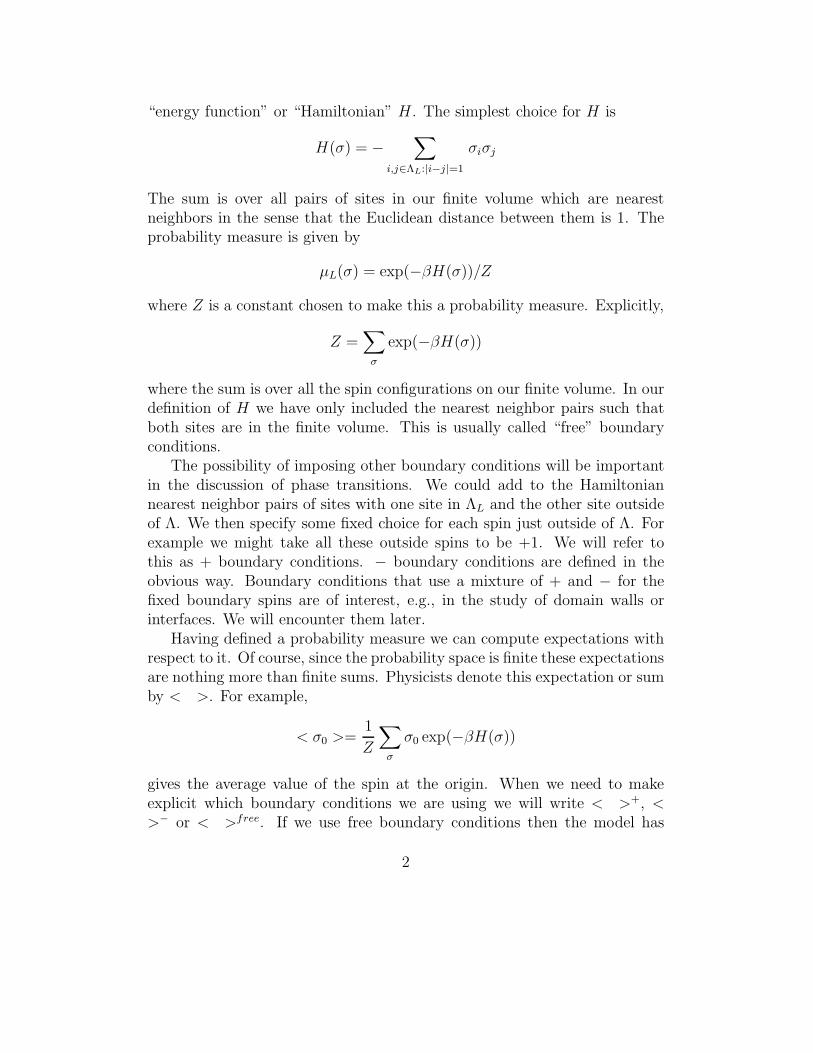
d. Then we let a → 0 instead of letting the volume grow. If thesystem has a finite correlation length then this correlation length will go tozero as we let a → 0. So the microspopic randomness in the system will notbe seen at macroscopic length scales. Figure 2 shows a typical domain wallfor β > βc (the low temperature phase). In the scaling limit the domain wallwill just be a straight line and so the same for almost all spin configurations.
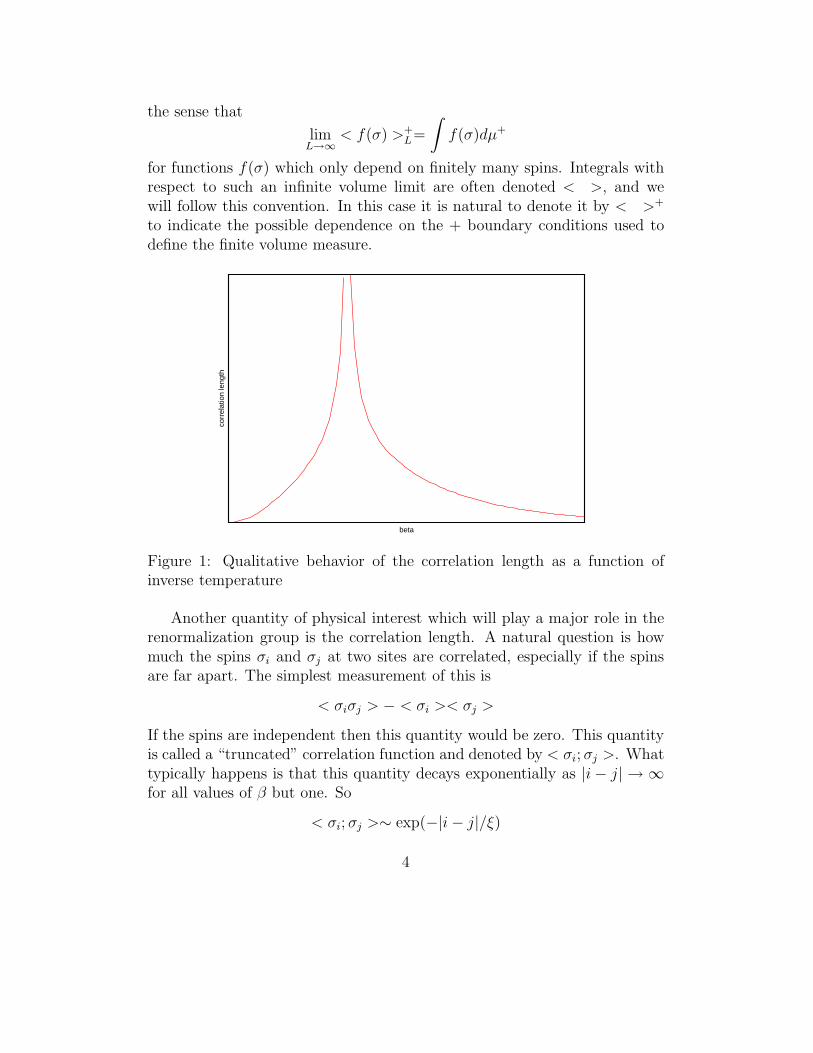
Figure 3 shows the domain wall when β = βc. Even in the scaling limitthe curve will be random. The fifth characterization of a critical point is thatthe microscopic randomness produces random structures on a macroscopic
22

0
100
200
300
400
500
600
0 100 200 300 400 500 600
Ising, beta=1.25*critical
Figure 2: Domain wall forced by mixed boundary conditions at β = 1.25βc.
scale.We end this crash course in critical phenomena with a brief discussion
of a different type of phase transition from those we have been considering.At the critical point T = Tc the second derivates of the free energy f withrespect to β and with respect to the magnetic field h both diverge, so f isnot analytic at the critical point. The first derivatives of f with respect toβ and h are both continuous functions. The phase transition at T = Tc iscalled a “second order” transition since second derivatives of the free energyare the lowest order derivatives which fail to be continuous. There are alsofirst order transitions in which first derivatives of the free energy fail to becontinuous.
We take the Ising model at very low temperature and consider the effect ofa small magnetic field. We have already seen that the effect of the boundaryconditions is quite dramatic - they produce two very different infinite volumelimits. If we take h > 0 then we will get an infinite volume limit in which< σ0 >> 0. What is more subtle is that if we take h > 0, take the infinitevolume limit and then let h → 0+ we will obtain a state < >h=0+ in whichthe expected value of σ0 is positive. In fact < >h=0+ is the same as < >+
the infinite volume state we get from + boundary conditions. Likewise wecan obtain < >− by imposing a negative h and taking h → 0− after we have
23

0
100
200
300
400
500
600
0 100 200 300 400 500 600
Ising, critical beta
Figure 3: Domain wall forced by mixed boundary conditions at β = βc.
taken the infinite volume limit. It is crucial that we let h → 0 only after wehave taken the infinite volume limit. Now consider the magnetization m asa function of h. (We are keeping the temperature fixed at some value belowTc.) As h → 0+, m will converge to < σ0 >+ while it converges to < σ0 >−
when h → 0−. Since < σ0 >+ and < σ0 >− are not equal, m has a jumpdiscontinuity at h = 0. This is a first order transition since a first derivativeof the free energy, namely the magnetization, is discontinuous.
First order transitions are quite different from second order ones. One ofthe most important differences is that the correlation length does not divergeas we approach the first order transition. Note also that there is actually anentire interval of first order transitions at h = 0 and 0 ≤ T ≤ Tc. The powerlaw divergences that we saw at second order transitions are not present atfirst order transitions, so there are no critical exponents associated with thefirst order transitions. First order transitions are simpler than second orderones and at very low temperatures there is a wonderful rigorous treatmentof first order transitions due to Pirogov and Sinai. There is a nice rigorousrenormalization group approach to this “Pirogov-Sinai” theory by Gawedski,Kotecky and Kupiainen.
Exercises:
24

1.3.1 (really easy) Show that the scaling laws hold for both the d = 2 Isingcritical exponents and for the mean field exponents, but the hyperscalinglaws only hold for the former.
25

Critical exponents
t = (T − Tc)/Tc
ν, correlation length :
ξ ∼ t−ν as t → 0, ν2d = 1, νMF = 1/2
γ, magnetic susceptibility :
χ =δm
δh= −δ2f
δh2∼ |t|−γ as t → 0, γ2d = 7/4, γMF = 1
α, specific heat :
C =δ2f
δβ2∼ |t|−α as t → 0, α2d = log, αMF = 0(disc.)
β, spontaneous magnetization :
m =δf
δh∼ (−t)β as t → 0−, β2d = 1/8, βMF = 1/2
δ, response to magnetic field at T = Tc:
|m| ∼ h1/δ as h → 0, δ2d = 15, δMF = 3
η, correlation function at Tc :
< σ0σx >∼ 1
|x|d−2+ηas |x| → ∞, η2d = 1/4, ηMF = 0
Scaling laws:
α + 2β + γ = 2
βδ = β + γ
Hyperscaling laws:
26

dν = 2 − α
2 − η = d(δ − 1)
(δ + 1)
See table on p. 111 of Goldenfeld for 3d values and experimental values.
27