1

TCOM 5143

Lecture 12

Financial Analysis Techniques

2

Time Value of Money

• Money has a value dependent on time. • ie. $1000 today is more valuable than $1000 a year

from now (why ??)

• Future Value - value of money at some point in the future

3

Cost of Capital

• Cost of capital or cost of money: minimum acceptable rate of return on an investment or project undertaken by the capital. It is sometimes estimated by the interest rate.

• Compare the cost of capital for Microsoft and CocaCola.

4

Depreciation

Depreciation is spreading the cost of equipment over a number of years. Designed to account for lowering of equipment value due to obsolecence, use etc.

Many methods used. One’s we will consider are:• Straight Line Dep. over a number of years, i.e.

equal amounts reduced over 3, 5 or 7 years• Accelerated Dep. - larger portion allocated over first

few years. Usually depreciation is calculated by schedule provided.

5

Straight Line Depreciation

• Depreciable cost = cost of equipment - Salvage value

• Depreciation amount per yearDepreciable cost / number of years

• Equal amounts depreciated each year

6

Basic Analysis Techniques

• Net Present Value (NPV) :• Sum of all future cash flows minus the initial cost• if NPV is positive then accept the project else

reject• if NPV of project A is greater than NPV of project

B then accept A (as long as both NPV’s are positive)

7

Cash Flows (Single Payments)

• Consider a loan of $ P to be paid back after n years at i % interest per annum• Future amount to be payed back F = P*(1+i)n

• Present value of future amount P = F/ (1+i)n

8

Cash Flows (Annuity)

• Making (or rec’ving) equal amounts of payment over a number of years

• Consider $A to be paid out at the end of each year for the next n years

• What would all these payments be worth after n years ? (future value F)• F = A(1+i)n-1 + ....... + A(1+i)1 + A

9

Cash Flows (Annuity)

• What would all these payments be worth today ? (present value P)• P = A/(1+i)1 + A/(1+i)2 + ...... + A/(1+i)n

10

Cash Flows (Variable Amounts)

• Consider nonequal amounts CF1, CF2 .... CFn to be paid out every year for n years • Present value:

• P = CF1/(1+i)1 + CF2/(1+i)2 + .... + CFn/(1+i)n

11

Computing Net Cash Flows:

• Net cash flow from project = Cash In - Cash Out

= Revenue - expenses other than depreciation - capital expenditure - income taxes

• income taxes=tax rate *(Revenue - expenses other than depreciation -depreciation)

12

Example 1:

• Consider a project for a small ATM network:• Initial outlay: $100,000, Cost of capital 10%

• Expenses : $50,000 each year for three years

• The equipment will be obsolete after 3 years and can be salvaged for $10,000

• Straight line depreciation for 3 years

• Revenues : $200,000 per year for 3 years

• Tax rate=50%

• The status quo is no revenues and no expenses

• Should the project be undertaken ??

13

Example (cont.)

Financial study for the project:

Summary

• Cost of capital 10%

• Tax rate 50%

• Initial cost $100 000

• Lifetime of the project 3 years

• Yearly expense $50 000

• Salvage value $10 000

• Yearly revenue $200 000

14

Example (cont.)• Revenue 200 000

• Expense other than depreciation (50 000)

• Taxes• Revenue -expense 150 000• Less depreciation (30 000) (=(100000-10000)/3)• Taxable Income 120 000

• Tax (60 000)

• Net Cash flow for a generic year 90 000

(=200 000-50 000-60 000)

15

Example (cont.)Year 1 year 2 year 3

Cash flow 90 000 90 000 100 000 (=90 000 +10

000)

Present value 81 818 74 380 75 131

NPV=(81 818+74 380+75 131)- 100 000=131 329.

Decision: Yes, undertake the project because NPV>0

16

Other methods:

• Internal Rate of Return: IRR method• At what rate must the same amount of money be

invested to obtain the same cash flows (as this project).

• If this rate is lower than that current banks give then dont invest in project

• Payback period method:• How long will it take for the project to payback its

investment ?

• Accounting Rate of Return :• ROI = Average Annual profit/initial expense

17

Incorporating Risk

• The previous model assumed every thing was certain (deterministic)

• The real world is not deterministic rather it is stochastic

• Every event has a chance (probability associated with it)

18

Factors or reasons of Uncertainties:• Smooth factors:

• Small variations in events:• interest rates

• traffic requirements

• project delays/cost overruns

• Singular or discontinuous factors:• Catastrophic events or majors alterations in operating

parameters• Fire/Flood/Hurricane/Earthquake

• Acquisition/merger

• Loss of vendor/product

19

Probability basics

• Notation:• Probability that event A will occur = P(A)

• P(A&B) = P(A)*P(B) if A and B are independent

• P(Aor B) = P(A) + P(B) - P(A & B)

• Sum of all probabilities of an event = 1

• P(A|B) = P(A&B)/P(B) if A and B are not independent

20

Expected Value

• For event X which takes on values x1, x2, x3 .....with probabilities p1, p2, p3 .....

• Expected value E(X) = x1*p1 + x2*p2 + x3*p3 .....

• Standard deviation:• the expected deviation from the expected value

= sqrt(E(X2) - (E(X)) 2)

• The lower the standard deviation, the better

21

Expected Value: Example

• Consider the following:• Revenue = $200,000 with probability 0.5

• Revenue = $150,000 with probability 0.25

• Revenue = $250,000 with probability 0.25

• Expected value of revenue = E(Revenue)= 200,000 * 0.5 + 150,000 *0.25 + 250,000 *0.25

= $200,000

22

Example 1 (cont.)

• Consider the following in example 1:• Revenues in Year 1 could be:

• $200,000 with probability 0.3

• $150,000 with probability 0.5

• $100,000 with probability 0.2

• Year2:• $250,000 with probability 0.3

• $200,000 with probability 0.5

• $150,000 with probability 0.2

23

Example 1 (cont.)

• Year3:• $250,000 with probability 0.3

• $200,000 with probability 0.5

• $150,000 with probability 0.2

• Expenses each year:• $ 70,000 with probability 0.5

• $60,000 with probability 0.3

• $50,000 with probability 0.2

• Does this change your choice to accept or reject this project ?

24

Example 1 (cont.)Year 1 Year 2 Year 3

E(revenue) 155 000 205 000 205 000

E(expense) 63 000 63 000 63 000

{Taxable income=revenue-expense-depreciation}

Taxable Income 62 000 112 000 112 000

Tax 31 000 56 000 56 000

{Cash flow=revenue -expense-tax}Cash flow 61 000 86 000 96 000

(86000+10000)

Present Value 55 455 71 074 72 126

25

Example 1 (cont.)

NPV= (55 455+71 074+72 126)-100 000

=98 655

Decision: Yes, undertake the project because NPV>0

26

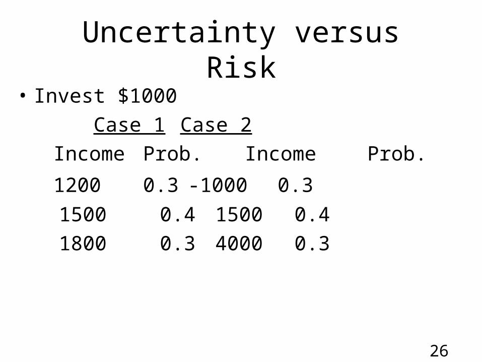
Uncertainty versus Risk

• Invest $1000

Case 1 Case 2

Income Prob. Income Prob.

1200 0.3 -1000 0.3

1500 0.4 1500 0.4

1800 0.3 4000 0.3

27

Forecasting

• Assumes causal system• ie. past ==> future

• Forecasts rarely perfect due to randomness

• Forecasts more accurate for large samples

• Forecast accuracy decreases as time horizon increases

28

Steps in Forecasting Process

• Determine purpose of forecast

• Establish a time horizon

• Select a forecasting technique

• Gather and analyze data

• Prepare the forecast

• Monitor the forecast

29

Types of Forecasts

• Judgemental• uses subjective inputs (eg. gut feeling that demand

for service A will skyrocket in next quarter)

• Time series • uses historical data (assuming future will be like

past)

30

Judgemental Forecasts

• Executive opinions

• Sales force composite

• Consumer Surveys

• Outside opinion

• Opinions of managers and staff

31

Time Series Forecasts

• Trend - long term movement in data

• Seasonality - short term regular variations in data

• Irregular variations - caused by unusual circumstances

• Random variations - caused by chance

32

Forecasting methods

• Averaging:• Calculate average over previous periods and apply

the same to future periods• Highly inaccurate in most cases

• Moving Average:• Calculate average over a restricted number of

previous periods (say 6 months) and use that for forecasting future periods

33

Forecasting methods

• Exponential smoothing:• Ft = Ft-1 + (At-1 - Ft-1)

• premise: the most recent observations might have the highest predictive value. Therefore give them the most weight. • Ft = forecast at time t

• At = actual value at time t

• = smoothing constant

34

Forecasting methods

• Regression:• Underlying trend is to be estimated and is assumed

to be of the form:• Y = a + b1X1 + b2X2 .....

• Y is value to be predicted

• X1, X2 ... are factors affecting outcome

• Goal is to fit a line to the set of points (samples) given

35

Simple regression

• Yi=a+bXi Yi

Xi

nXXn

ii /][

1

nYYn

ii /][

1

n

ii

n

iii

XnX

YXnYXb

1

22

1

XbYa

36

Simple regression: ExampleA credit card company has installed a client/server system in each of its 9 credit processing centers. For each center, the company collected data about the # of users and the budget. The company wants to estimate the budget for a new center with 50 users.#of users budget34 2137 2438 2539 2542 2843 2645 2946 2848 31

37

Example (cont.)X Y XY X2

34 21 714 115637 24 888 136938 25 950 144439 25 975 152142 28 1176 176443 26 1118 184945 29 1305 202546 28 1288 211648 31 1488 2304

sum 372 237 9902 15548

38

Example (cont.)

41.33372/9 nXXn

ii

/][1

705.033.41*62.033.26 XbYa

if X=50 then Y=0.705+0.62*50=31.705

.3362237/9 /][1

nYYn

ii

62.0)33.41(*915548

33.26*33.41*999022

1

22

1

n

ii

n

iii

XnX

YXnYXb