1

Subionospheric VLF propagation

Prepared by Morris Cohen, Benjamin Cotts, Forrest FoustStanford University, Stanford, CA

IHY Workshop on Advancing VLF through the Global AWESOME Network

2N. Lehtinen

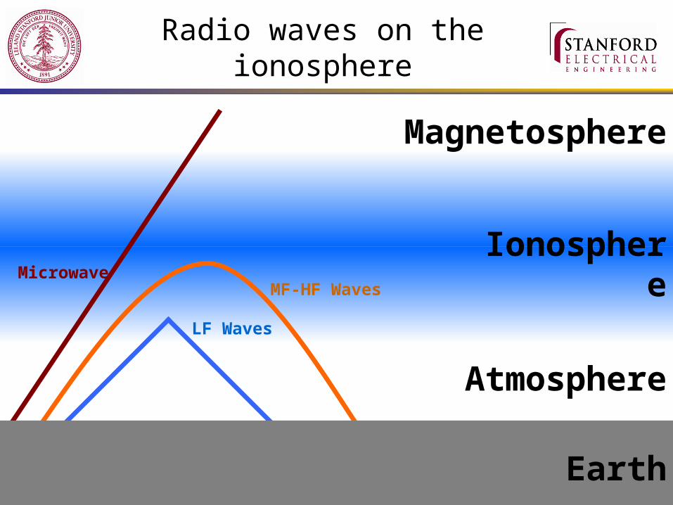
Radio waves on the ionosphere

MicrowaveMF-HF Waves

LF Waves

Earth

Ionosphere

Atmosphere

Magnetosphere

3

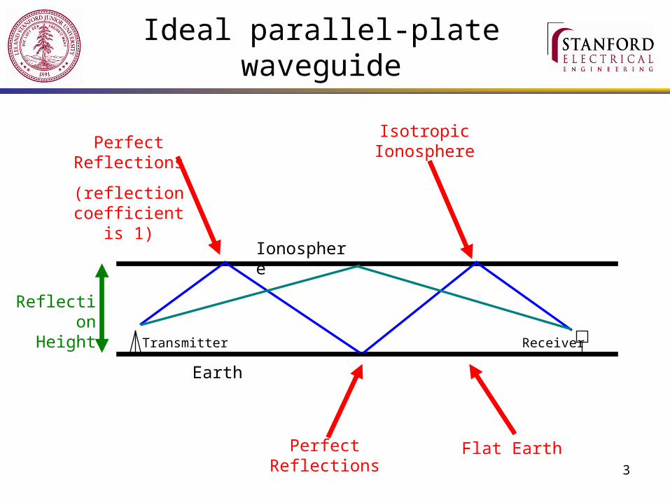
Ideal parallel-plate waveguide

Reflection Height

Earth

Ionosphere

Transmitter Receiver

Perfect Reflections

(reflection coefficient is 1)

Perfect Reflections

Flat Earth

Isotropic Ionosphere

4

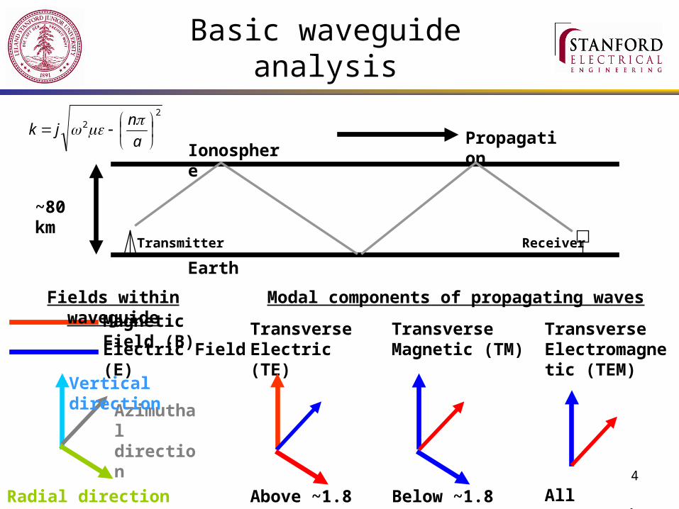
Basic waveguide analysis

~80 km

Transverse Electric (TE)

Transverse Magnetic (TM)

Magnetic Field (B)Electric Field (E)

Radial direction (propagation)

Azimuthal direction

Fields within waveguide

Modal components of propagating waves

Vertical direction

Above ~1.8 kHz

Below ~1.8 kHz

Earth

Ionosphere

Propagation

Transmitter

Receiver

Transverse Electromagnetic (TEM)

All Frequencies

22

a

njk

5

Typical Spectrogram

TEM Wave

Weak TEM

TE and TM

6

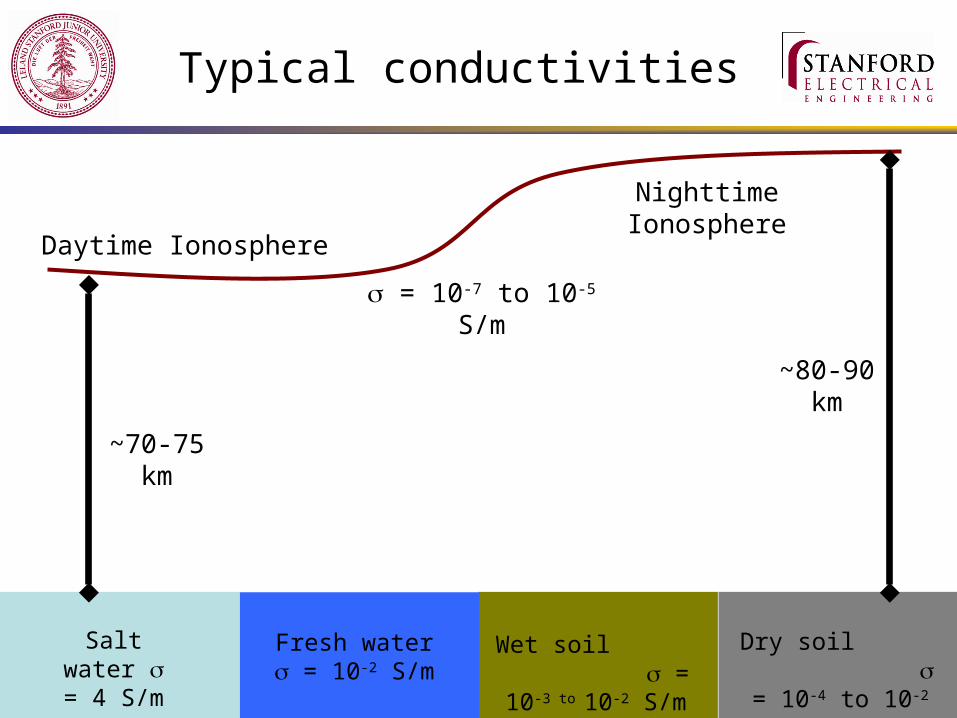
Typical conductivities

Salt water = 4 S/m

Fresh water = 10-2 S/m

Dry soil = 10-4 to 10-2 S/m

Wet soil = 10-3 to 10-2 S/m

= 10-7 to 10-5 S/m

Daytime Ionosphere

~70-75 km

~80-90 km

Nighttime Ionosphere

7

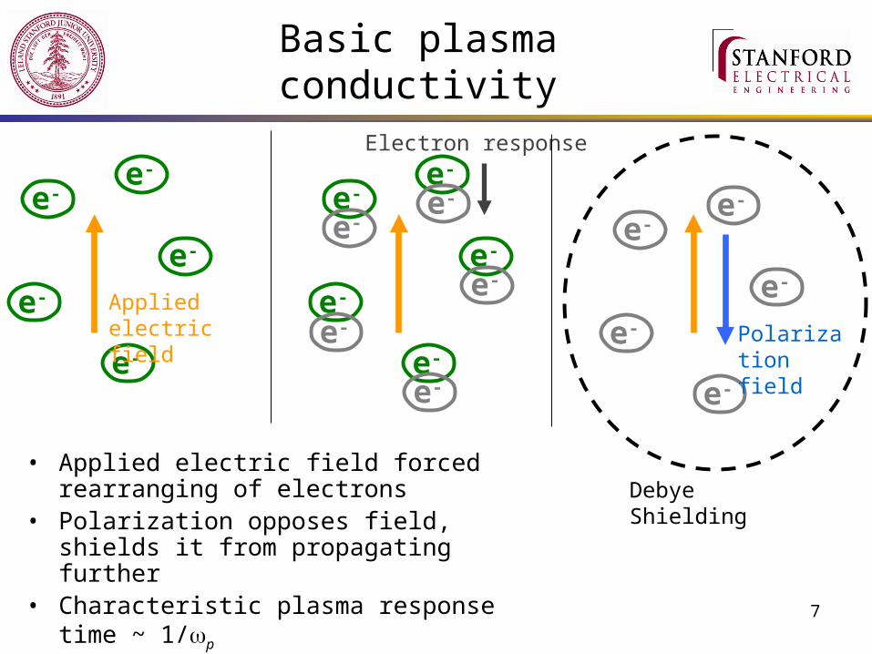
Basic plasma conductivity

e-

e-

e-

e-

e-

e-

e-

e-

e-

e-

e-

e-

e-

e-

e-

Applied electric field

e-

e-

e-

e-

e-

Electron response

Polarization field

Debye Shielding• Applied electric field forced rearranging of

electrons• Polarization opposes field, shields it from

propagating further• Characteristic plasma response time ~ 1/p

p2 ~ Ne

8

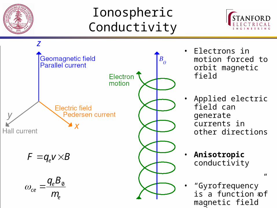
Ionospheric Conductivity

BvqF e

xy

z• Electrons in motion

forced to orbit magnetic field

• Applied electric field can generate currents in other directions

• Anisotropic conductivity

• “Gyrofrequency” is a function of magnetic field and e- mass

e

ece m

Bq 0

9

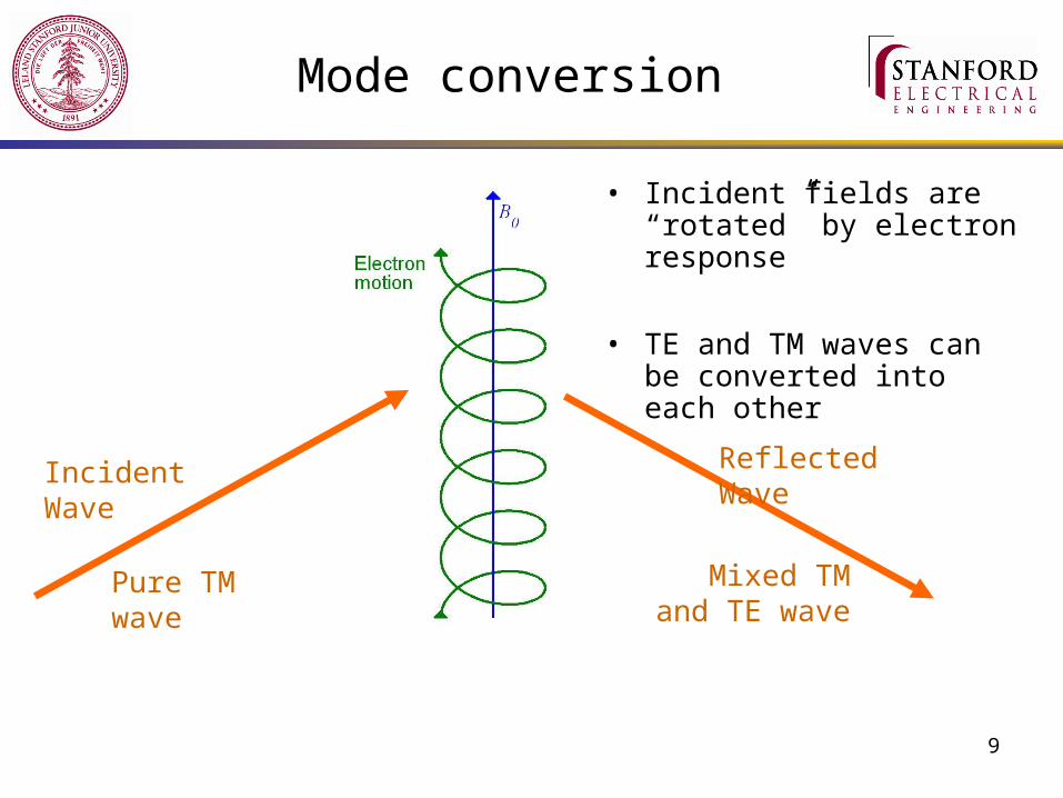
Mode conversion

• Incident fields are “rotated” by electron response

• TE and TM waves can be converted into each other

Incident Wave Reflected Wave

Pure TM wave Mixed TM and TE wave

10

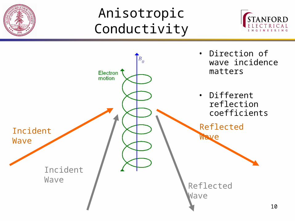
Anisotropic Conductivity

• Direction of wave incidence matters

• Different reflection coefficients

Incident Wave Reflected Wave

Incident Wave

Reflected Wave

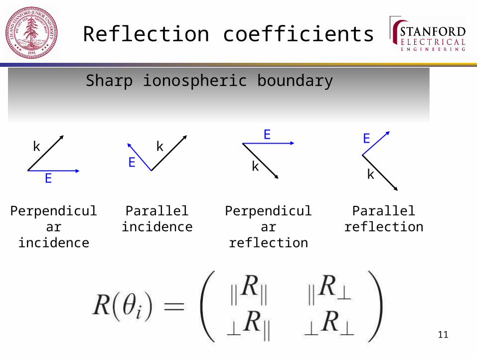
11

Sharp ionospheric boundary

E

k

Perpendicular incidence

Ek

Parallel incidence

E

k

Perpendicular reflection

E

k

Parallel reflection

Reflection coefficients

12

Example

13

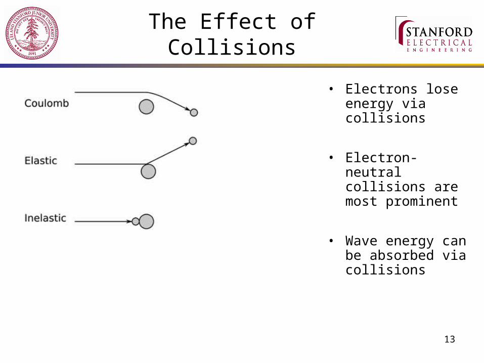
The Effect of Collisions

• Electrons lose energy via collisions

• Electron-neutral collisions are most prominent

• Wave energy can be absorbed via collisions

14

Collisions and Magnetic Field

• Lower D-region, collision frequency much higher than gyrofrequency• Higher altitudes, collisions rare, magnetic field dominates

• Plasma frequency (electron density) increasing rapidly

Dominated by Collisions

Dominated by Magnetic Field

p= c

15

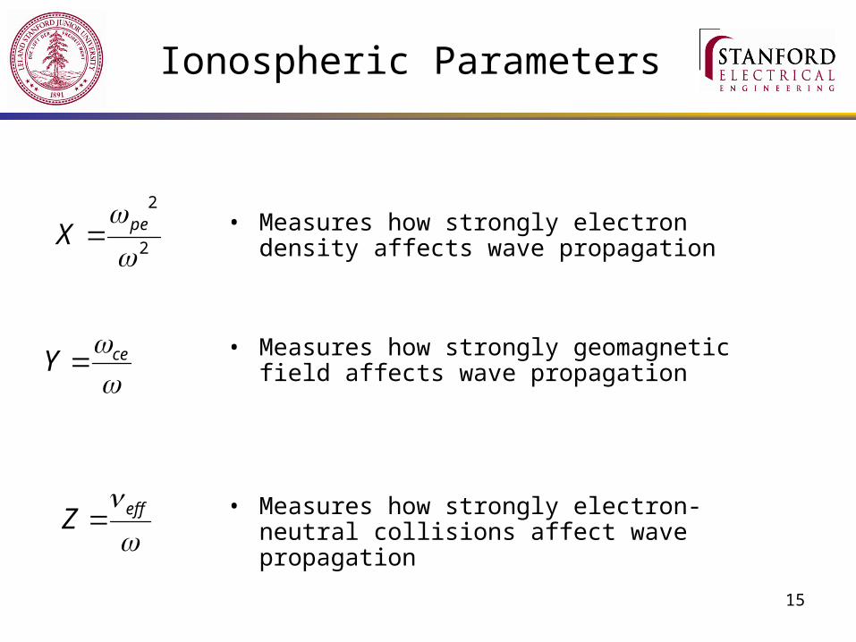
Ionospheric Parameters

• Measures how strongly electron density affects wave propagation2

2

peX

ceY

effZ

• Measures how strongly geomagnetic field affects wave propagation

• Measures how strongly electron-neutral collisions affect wave propagation

16

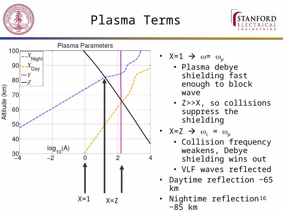
Plasma Terms

X=1 X=Z

• X=1 = p

• Plasma debye shielding fast enough to block wave

• Z>>X, so collisions suppress the shielding

• X=Z c = p

• Collision frequency weakens, Debye shielding wins out

• VLF waves reflected• Daytime reflection ~65 km• Nightime reflection ~85 km

17

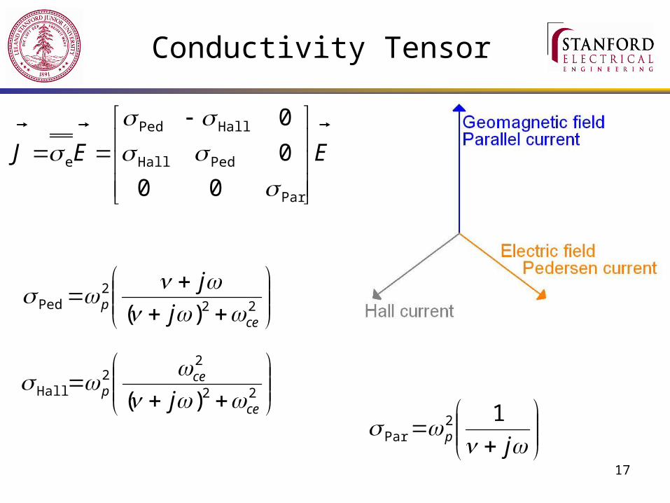
Conductivity Tensor

EEJ

Par

PedHall

HallPed

e

00

0

0

222

Ped )( cep j

j

22

22

Hall )( ce

cep j

jp

12Par

18

Ionospheric Changes

Daytime Ionosphere

~70-75 km

~80-90 km

Nighttime Ionosphere

TransmitterReceiver

Earth

Scattered Wave

Incident Wave

Reflected Wave

Mode conversion

19

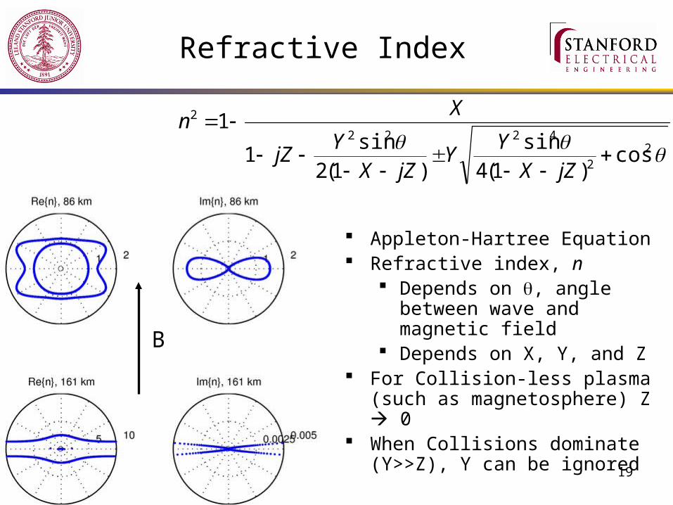
Refractive Index

22

4222

2

cos)1(4

sin)1(2

sin1

1

jZXY

YjZX

YjZ

Xn

B

Appleton-Hartree Equation Refractive index, n

Depends on , angle between wave and magnetic field

Depends on X, Y, and Z For Collision-less plasma (such

as magnetosphere) Z 0 When Collisions dominate

(Y>>Z), Y can be ignored

20

“Helliwell” Absorption assumption Normal incidence Wavelength is much smaller than the size of any variation in the medium.

Loss () is proportional to the imaginary part of the refractive index

(in dB)

Ionospheric Absorption

1

1)Im(69.8 dzc

n

21

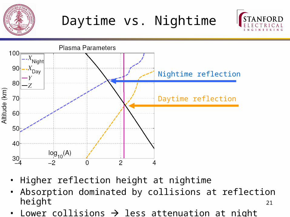
Daytime vs. Nightime

Nightime reflection

Daytime reflection

• Higher reflection height at nightime• Absorption dominated by collisions at reflection height• Lower collisions less attenuation at night

22

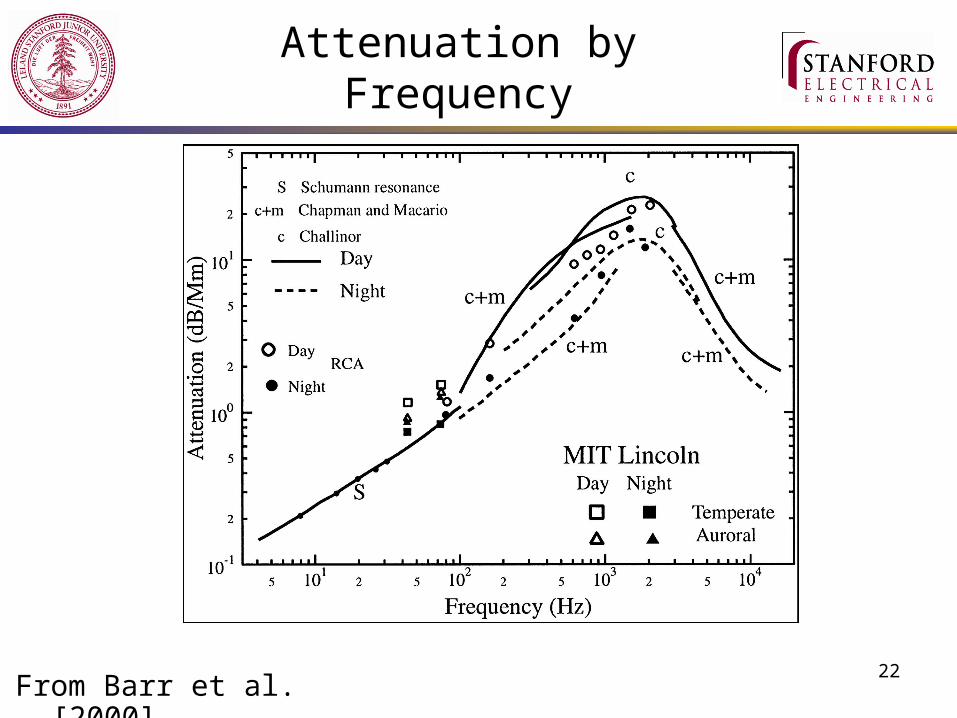
Attenuation by Frequency

From Barr et al. [2000]

23

References

• K.G. Budden, The Wave-Guide Mode Theory of Wave Propagation, 1961, Prentice Hall

• J.R. Wait, Electromagnetic Waves in Stratified Media, 1962, Pergamon Press.

• J. Galejs, Terrestrial Propagation of Long Electromagnetic Waves,1972 Pergamon Press

• R.A. Helliwell, Whistlers and Related Ionospheric Phenomena, 1965

• R. Barr et al., ELF and VLF Radio Waves, J. Atmos. Sol.-Terr. Phy., Vol.2,1689-1719, 2000.