Embed Size (px)
Citation preview

1. Stellar Rotation
The gravitational force ~Fg is related to the gravitational potential φg by
~Fg = −∇φg , (1)
where ∇ is the gradient operator, which in Cartesian coordinates is
∇ =∂
∂xi +
∂
∂yj +
∂
∂zk (2)
For a spherically symmetric mass distribution the gravitational potential is just
φg = −G Mr
r, (3)
but if rotation breaks that symmetry, φg will not be so simple. In any case, the potential is
related to the mass distribution through the Poisson equation
∇2φg = 4πGρ , (4)
where ∇2 is the Laplacian
∇2 =∂2
∂x2+
∂2
∂y2+
∂2
∂z2. (5)
Under the assumption that our star is rotating as a rigid body with an angular velocity
ω, the velocity at any point is v = ωa, where a is the distance from the axis of rotation (the
z axis)(NB. a is not acceleration!). The centrifugal force is ~Fc = (v2/a)a, that is
~Fc = ω2a a = ω2 (x2 + y2)1/2 a. (6)
We see that this force can be obtained from the potential φc:
φc = −1
2ω2 (x2 + y2) . (7)
Thus the total force F acting on a mass element in the star is
~F = ~Fg + ~Fc = −∇φ where φ = φg + φc . (8)
Now we see that ∇2φc = − 2ω2 , so that the Laplacian of the total potential φ is
∇2φ = 4πGρ − 2ω2 . (9)
We now introduce the more general form of the equation of hydrostatic equilibrium:
∇P = − ρ ∇φ . (10)
You can see that in the absence of rotation, this just becomes the familiar dP/dr = −ρg.
1

Now ∇P and ∇φ are both vectors while ρ is a scalar. Thus ∇P must be parallel to
∇φ. If we move along a surface of constant φ, then P will also remain constant along this
surface. Since P can only change with φ, the pressure can be written as a function of φ only:
P = P (φ). But then, since
∇P (φ)
∇φ= − ρ , it follows that ρ = ρ(φ) . (11)
The equation of state for densities where we need only consider ideal gas pressure and
radiation pressure is
P (φ) =NAk
µρ(φ) T +
1
3arad T 4 (12)
If we assume that the mean molecular weight µ is constant, or that it is a function of potential
only, µ = µ(φ), then we see that all the variables in equation (12) other than T are functions
of φ only. Thus we must also have T = T (φ). So we conclude that all the variables P ,ρ, and
T are constant along equipotential surfaces.
Next, let us consider the equation for radiative energy transport:
~F = −4c arad
3
T 3
κρ∇T (13)
Now, since T is a function of φ only, we can write the gradient as
∇T =∂φ
∂x
dT
dφi +
∂φ
∂y
dT
dφj +
∂φ
∂z
dT
dφk =
dT
dφ∇φ (14)
Thus
~F =
−4c arad
3
T 3
κρ
dT
dφ
∇φ (15)
The expression is braces is a function of φ only, so we can write
~F = f(φ) ∇φ where f(φ) =
−4c arad
3
T 3
κρ
dT
dφ
(16)
Now we turn to the equation of thermal equilibrium. The usual equation of stellar
structure isdF
dr= ρǫ , (17)
where ǫ is the nuclear energy generation rate. (A more familiar form is obtained if we recall
that 4πr2F = Lr). The 3-dimensional generalization of this equation involves the divergence
of the radiative flux:
∇ · ~F = ρǫ (outside the core: ∇ · ~F = 0) (18)
Now
∇ · ~F =∂Fx
∂x+
∂Fy
∂y+
∂Fz
∂z(19)
2

Fig. 1.— The coordinate system for a rotating star.
Fig. 2.— Equipotential surfaces of a rotating star (schematic).
3

Using equation (16) for the flux and noting that the x-component of ∇φ is ∂φ/∂x i etc.,
we see that
∇ · ~F =
[
∂f
∂x
∂φ
∂x+ f
∂
∂x
(
∂φ
∂x
)]
+
[
∂f
∂y
∂φ
∂y+ f
∂
∂y
(
∂φ
∂y
)]
+
[
∂f
∂z
∂φ
∂z+ f
∂
∂z
(
∂φ
∂z
)]
(20)
∇ · ~F =
[(
∂f
∂φ
∂φ
∂x
)
∂φ
∂x+ f
∂2φ
∂x2
]
+ · · · (21)
∇ · ~F =
[
∂f
∂φ
(
∂φ
∂x
)2
+ f∂2φ
∂x2
]
+ · · · (22)
and combining the x,y and z components, we obtain
∇ · ~F =∂f
∂φ|∇φ|2 + f ∇2φ (23)
We now insert the value of the Laplacian from equation (9):
∇ · ~F =∂f
∂φ|∇φ|2 + f
(
4πGρ− 2ω2)
. (24)
With this expression for the divergence we return to equation (18) and obtain
∂f
∂φ|∇φ|2 + f
(
4πGρ− 2ω2)
= ρǫ . (25)
Examination of this equation shows that everything except for ∇φ is a function of φ only,
i.e., constant over a surface of constant φ. That is, if we travel along an equipotential surface
while θ varies from 0 to π, everything except ∇φ remains constant. On the other hand, ∇φ
does vary with θ. Looking at Fig. 2, we see that the surfaces are closer together at θ = 0
and further apart at θ = π/2. This means that ∇φ is greater in the polar direction (along
the z-axis) than in the equatorial direction. The only way to reconcile these restrictions is if
df
dφ= 0 which implies that f = constant (26)
As a result we see that
ρǫ = f(
4πGρ− 2ω2)
(27)
And since f is constant we can write this as
ǫ = constant
(
1−ω2
2πGρ
)
(28)
This result is known as von Zeipel’s paradox (von Zeipel 1924). For how can the rate of
nuclear energy generation ǫ be directly determined by the angular velocity of the star’s
rotation? This is not possible, so what we have proved is that a uniformly rotating star
cannot be in radiative thermal equilibrium.
4

What may happen is that, in regions outside the core where we should have ∇· ~F = 0 ,
we will instead have
∇ · ~F =∂f
∂φ|∇φ|2 + f
(
4πGρ− 2ω2)
6= 0 . (29)
The divergence of the radiative flux will be positive in some directions and negative in
others, which will cause heating or cooling, which in turn may lead to slow currents within
the star which will balance this excess heating or cooling. These currents are known as
Eddington-Sweet currents. See Fig. 3. Now the currents will not be very fast, so the
equation of hydrostatic equilibrium (equation 10) will be obeyed closely. And all the steps
in the derivation will hold up to equation (16), but now we can’t have f(φ) strictly constant
from one φ to the next. But consider some equipotential surface φ0 just under the surface.
Over this surface~F = f(φ0) ∇φ = f0 ~g (30)
and this must be continuous with the radiation escaping from the atmosphere. Here recall
that the gradient of the total potential φ is just ~g, the effective gravity, i.e., the gravity minus
the centrifugal acceleration. This behavior ( ~F ∝ ~g) is called “gravity darkening” since the
stellar surface near the equator, where the effective gravity is small, will have a reduced flux
and will thus be “darker”. The scalar form of this relation,
F ∝ g =⇒ Teff ∝ g1/4 (31)
is referred to as “von Zeipel’s law”. Thus a rapidly rotating star will have a surface temper-
ature which varies with latitude, highest at the pole and lowest at the equator.
2. The Shape of Rotating Stars
Going back to the total potential
φ = φg −1
2ω2 a2 (32)
where a = (x2 + y2)1/2 , the distance from the z-axis. Most stars are rather centrally
condensed, so we can justify adopting a Roche model, that is, a model with all the mass
concentrated in the center. Then we can approximate φg by the potential of a spherical
distribution
φg = −GMr
r(33)
so at the surface the potential is
φ = −GM
r−
1
2ω2 a2 (34)
and the local gravity is
~g = −∇φ = −GM
r2r + ω2a a (35)
5

Fig. 3.— Eddington-Sweet currents outside a convective core.
6

At the pole a = 0 while at the equator a = r.
What is the break-up rotational velocity of the star? We seek the critical ωc such that
g = 0 at the equator. Thus, if re is the equatorial radius,
g = 0 = −GM
r2e+ ω2
cre (36)
ω2
c =GM
r3e=⇒ ωc =
(
GM
r3e
)1/2
(37)
But we don’t know what re is, since the star stretches out! Now the pole is on the same
potential surface as the equator. Thus, if rp is the polar radius,
−GM
rp= −
GM
re−
1
2ω2
c r2e (38)
−GM
rp= −
GM
re−
1
2
(
GM
r3e
)
r2e = −3
2
GM
re(39)
Thus we see that
re =3
2rp for ω = ωc (40)
Further, the rotational velocity of the equator at break-up is
vc = re ωc =
(
GM
re
)1/2
=
(
2
3
GM
rp
)1/2
(41)
Now we may be tempted to argue that rp won’t change with a star’s rotation – after all, the
gravity along the z-axis doesn’t change. (This sounds reasonable, but is only approximately
true.) We will assume it’s OK.
So what is the break-up velocity of the sun? Put rp = R⊙ and M⊙ into equation (41) and
we find vc = 357 km/s, which corresponds to a period of P = 3π rp/ve = 5.1 hr. Actually,
the sun’s rotation is much slower, ve = 2 km/s, P = 25 days. Over 4 billion years, the
sun has lost most of its angular momentum to the solar wind, to which it is magnetically
coupled.
Here are some examples of break-up velocities:
Type M/M⊙ vc km/s Period
Main Sequence 1 357 5.1 hr
3 456 7.3 hr
5 507 8.9 hr
10 584 11.6 hr
White Dwarf 1.0 4000 13.1 sec
Neutron Star 1.4 100000 0.001 sec
If we define a scaled radius x(θ, w) = R(θ, ω)/Rp, then it is easy to see that the require-
ment that all points on the star lie on the same equipotential surface as the pole (where
7

x = 1) leads to a cubic equation for x:
4
27(w sin θ)2 x3 − x + 1 = 0 , (42)
where w is the angular velocity in terms of the critical velocity, w = ω/ωc. Thus the shape
function x may be written, using the trigonometric form of the solution of the cubic equation,
as:
x(θ, w) =3
w sin θcos
1
3[π + arccos(w sin θ)]
(43)
Here are some equatorial to polar ratios for various values of w:
w = ω/ωc x(π/2, w) = Re/Rp
0.5 1.042
0.8 1.141
0.9 1.216
0.95 1.281
0.99 1.390
1.0 1.5
The next figure shows the shapes obtained from this equation for various values of w.
To obtain the value of the effective gravity, we must remember that the two components in
equation (35) are not parallel. If we take a coordinate axis η perpendicular to the z-axis in
the plane of our point, this is the direction of the centripetal force. We can resolve the first
term into components:
−GM
r2r = −
GM
x2 R2p
[sin θ η + cos θ z] (44)
Thus the effective gravity can be written
~g =
[
−GM
x2 R2p
+ ω2 x Rp
]
sin θ η +
[
−GM
x2 R2p
]
cos θ z (45)
and the magnitude of the effective gravity as a function of θ follows from g = |~g| = (~g ·~g)1/2 :
g =
[
GM
x2 R2p
]
cos2 θ + sin2 θ
[
1 − ω2x3 R3
p
GM
]21/2
(46)
From equations (37) and (39) we see that ω2
c = (2/3)3 GM/R3
p, and using ω2/ω2
c = w2 we
obtain
g =
(
GM
R2p
)
1
x2
cos2 θ + sin2 θ
[
1 −8
27x3 w2
]21/2
. (47)
The figure shows the variation of gravity with latitude for a number of rotational veloc-
ities. As mentioned above, the surface brightness is proportional to the gravity, while the
surface temperature varies as the fourth root of the local effective gravity. These effects have
in fact been measured in nearby rapidly rotating stars such as Regulus and Vega.
8

Fig. 4.— The shapes of rapidly rotating stars from equation (42).
Fig. 5.— The variation of surface gravity for various rotational velocities.
9

3. The Surface Area and Temperature of a Rotating Star
While we might adopt the relative variation of surface temperature with latitude from von
Zeipel’s “law” (equation 31), we do not know the zero point: e.g., what is the temperature
of the pole? Compare the rotating star to a spherical non-rotating star of the same mass. If
the pole has the same temperature as the non-rotating star, then as the temperature drops
towards the equator, less flux will be radiated and the luminosity of the rotating star will
be lower than that of its static counterpart. (The area of the rotating star will be larger
than that of the spherical star, but as we will see, that is not enough to compensate for the
gravity darkening.) Lets look at this for the Roche model. The coordinates and angles for
our discussion are shown in Figs. 6 and 7. Any cross-section through the rotation axis will
slice out a plane Zη and we see that for any co-latitude θ, the unit normal to the surface, n,
makes an angle δ with the Z-axis. What is the angle δ ? We look at the η and Z components
of the local gravity (from equation 44):
~g =
[
−gpx2
+ ω2 x Rp
]
sin θ η +
[
−gpx2
]
cos θ z , (48)
where gp = GM/Rp2 is the magnitude of the gravity at the pole. Clearly the ratio of the η
component to the Z component is tan δ. Thus
tan δ =
1 −ω2x3Rp
gp
tan θ (49)
Now the last term in the braces is just
ω2x3Rp
gp= ω2
R3
px3
GM=
ω2
ω2c
8
27x3 =
8
27x3w2 (50)
(see p 8) so that we obtain
tan δ =
1 −8
27x3w2
tan θ . (51)
Note that when taking the arctan to obtain δ, we need to make sure δ is in the same quadrant
as θ. (See Fig. 8.)
Now to obtain the surface area of the star, we integrate‘ over the range 0 ≤ φ ≤ 2π and
0 ≤ θ ≤ π. The element of area in the radial direction r is just
dA′ = R(θ, w)2 dφ sin θ dθ = R2
p x(θ, w)2 dφ sin θ dθ (52)
with x(θ, w) from equation (43). There is no φ dependence, so we can do that integration.
Now the stellar surface element dA is inclined to the radial surface element dA′ by the angle
θ− δ, so dA projects onto dA′ by a factor of n · r = cos(θ− δ). Thus we must divide by this
factor:
A =
∫ ∫
dA = 4π R2
p
1
2
∫ π
0
x(θ, w)2sin θ
cos(θ − δ)dθ (53)
10

Fig. 6.— The coordinate systems defining the angles used in the text.
Fig. 7.— Cross-section of star in the Zη plane, defining angle δ.
11

We can then carry out the integration over θ numerically to find the surface area A of the
star. We provide some results in the table below.
The luminosity of our rotating star will be given by the flux from each surface element
integrated over the star. From equation (31), F = σT 4
eff (θ) ∝ g(θ), but von Zeipel’s relation
does not give us the constant of proportionality. If, however, we assign the temperature at
one point, e.g., the pole, then we can write
L =
∫ ∫
F dA = 2π R2
p σT 4
pole
∫ π
0
x(θ, w)2sin θ
cos(θ − δ)
[
T (θ)
Tpole
]4
dθ (54)
Now[
T (θ)
Tpole
]4
=g(θ)
gpole=
1
x2
cos2 θ + sin2 θ
[
1 −8
27x3 w2
]21/2
(55)
by equation (47). The x’s cancel leaving us with
L = 4π R2
p σT 4
pole
1
2
∫ π
0
sin θ
cos(θ − δ)
cos2 θ + sin2 θ
[
1 −8
27x3 w2
]21/2
dθ (56)
The leading term, 4π R2
p σT 4
pole, is just the luminosity of a spherical star of radius Rp and
surface temperature Tpole. The remaining integral thus gives the ratio of the luminosity
of a rotating star with polar radius Rp to a non-rotating star of radius Rp and surface
temperature Tpole. Some results are given in the table below. We see that the total luminosity
of the rotating stars will be substantially less than the non-rotating counterpart if the polar
temperature is held to that of the non-rotating star.
On the other hand, we might consider the proposition that the luminosity of the star
(which we might think is not much affected by the distortion of the outer envelope) should re-
main constant. Now if we simply increase the temperature for all θ by a factor (Lsphere/L)1/4,
then the luminosity will remain unchanged. This factor, which is just Tpole/Tsphere, is given
in the last column.
w = ω/ωc A/Asphere L/Lsphere Tpole/Tsphere
0.5 1.056 0.9465 1.0139
0.8 1.186 0.8375 1.0453
0.9 1.282 0.7705 1.0674
0.95 1.363 0.7222 1.0848
0.99 1.485 0.6645 1.1076
1.0 1.577 0.6394 1.1183
We should emphasize that we are simply assuming a constant polar radius and luminosity.
This is just a toy model; there are much more complex studies which do in fact find modest
decreases in luminosity and changes in polar radius. Further, we know that the assumption of
rotation with a uniform angular velocity ω is violated. We will return to this later. For now,
we want a simple model to investigate the effects of rotation on the variation of apparent
12

luminosity with viewing angle and the degree of polarization of the star’s radiation resulting
from the star’s non-spherical shape.
3.1. Beyond von Zeipel: A Improved Gravity Darkening Relation
We noted above that the von Zeipel law (eq. 31) neglects effects of the Eddington-Sweet
curents. Observations of nearby rapid rotators with stellar interferometers have found that
the von Zeipel law overestimates the temperature contrast between the pole and equator.
While modeling of rotating stars is very difficult (e.g., Rieutord and Espinosa Lara 2009),
some models have been computed and the resulting gravity darkening differs from the von
Zeipel law.
In light of these results, Espinosa Lara and Rieutord (2011) have presented a method
of computing an improved gravity darkening law based on the assumption that the flux
throughout the star is antiparallel to the effective gravity. They show that the the darkening
law can be obtained by solving one trancendental equation. They define
τ =1
3ω2r3 cos3 θ + cos θ + ln tan
θ
2(57)
where θ is the co-latitude and r = r/Req. They assume that the star is centrally condensed
so that the shape will be given by the Roche model. In terms of x(θ, w) (eq 43), r =
x(θ, w)/x(π/2, w). In these equations, the angular velocity ω is defined as Ω/Ωk, where Ωk
is the Keplerian angular velocity at the star’s equator, (GM/R3
e)1/2. Note that ω is not the
same as w: w is defined in terms of the break-up velocity of the star, while ω is in terms of
the Keplerian velocity at the equator of the star which is in gereral not at break-up velocity.
In fact,
ω =
[
2
3x(w,
π
2)
]3/2
w (58)
Having evaluated τ (eq 57), Espinosa Lara and Rieutord show that we only need solve
τ = cosΘ + ln tanΘ
2(59)
for Θ. Then the deviation from the von Zeipel law is given by the the quatity
Fω(θ) =tan2 Θ
tan2 θso that Teff (θ) ∝ (Fω(θ) g(θ))
1/4 (60)
This expression for Fω breaks down at the pole and equator; for these points we have
Fω(θ = 0) = e2
3ω2r3 and Fω(θ = π/2) = (1− ω2r3)−2/3 (61)
While the results of this formulation approachs the von Zeipel law for low angular ve-
locities (w < 0.5) it differs a great deal from von Zeipel for high angular velocities. For
example, at w = 0.7 (ω = 0.925723), the ratio Teq/Tp is 0.75737 for the von Zeipel g1/4 law
but 0.812208 for the Espinosa Lara and Rieutord formula. For w = 0.9 (ω = 0.992807), the
ratios are 0.556993 vs. 0.699711. (Also see Fig. 10.)
13
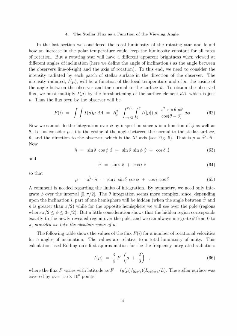
4. The Stellar Flux as a Function of the Viewing Angle
In the last section we considered the total luminosity of the rotating star and found
how an increase in the polar temperature could keep the luminosity constant for all rates
of rotation. But a rotating star will have a different apparent brightness when viewed at
different angles of inclination (here we define the angle of inclination i as the angle between
the observers line-of-sight and the axis of rotation). To this end, we need to consider the
intensity radiated by each patch of stellar surface in the direction of the observer. The
intensity radiated, I(µ), will be a function of the local temperature and of µ, the cosine of
the angle between the observer and the normal to the surface n. To obtain the observed
flux, we must multiply I(µ) by the foreshortening of the surface element dA, which is just
µ. Thus the flux seen by the observer will be
F (i) =
∫ ∫
I(µ)µ dA = R2
p
∫ π/2
−π/2
∫ π
0
I(|µ|)|µ|x2 sin θ dθ
cos(θ − δ)dφ (62)
Now we cannot do the integration over φ by inspection since µ is a function of φ as well as
θ. Let us consider µ. It is the cosine of the angle between the normal to the stellar surface,
n, and the direction to the observer, which is the X ′ axis (see Fig. 6). That is µ = x′ · n .
Now
n = sin δ cosφ x + sin δ sinφ y + cos δ z (63)
and
x′ = sin i x + cos i z (64)
so that
µ = x′ · n = sin i sin δ cosφ + cos i cos δ (65)
A comment is needed regarding the limits of integration. By symmetry, we need only inte-
grate φ over the interval [0, π/2]. The θ integration seems more complex, since, depending
upon the inclination i, part of one hemisphere will be hidden (when the angle between x′ and
n is greater than π/2) while for the opposite hemisphere we will see over the pole (regions
where π/2 ≤ φ ≤ 3π/2). But a little consideration shows that the hidden region corresponds
exactly to the newly revealed region over the pole, and we can always integrate θ from 0 to
π, provided we take the absolute value of µ.
The following table shows the values of the flux F (i) for a number of rotational velocities
for 5 angles of inclination. The values are relative to a total luminosity of unity. This
calculation used Eddington’s first approximation for the the frequency integrated radiation:
I(µ) =3
4F
(
µ +2
3
)
, (66)
where the flux F varies with latitude as F = (g(µ)/gpole)(Lsphere/L). The stellar surface was
covered by over 1.6× 10⁶ points.
14

w = ω/ωc i = 0o i = 15o i = 30o i = 45o i = 60o i = 75o i = 90o
0.5 1.0745 1.0670 1.0466 1.0187 0.9907 0.9702 0.9627
0.8 1.2626 1.2365 1.1648 1.0662 0.9672 0.8946 0.8680
0.9 1.4114 1.3707 1.2588 1.1041 0.9484 0.8345 0.7929
0.95 1.5401 1.4871 1.3405 1.1369 0.9320 0.7824 0.7279
0.99 1.7260 1.6556 1.4595 1.1842 0.9062 0.7071 0.6343
1.0 1.8225 1.7435 1.5222 1.2082 0.8945 0.6682 0.5861
We see that for this model, a star rotating at 95% break-up will appear twice as bright
when viewed from the pole as when viewed from the equator. This effect should be considered
when rapidly rotating stars are placed on the H-R diagram.
5. The Net Polarization of Radiation from Rotating Stars
In stellar atmospheres where the scattering (either by free electrons or by molecules) is
a substantial fraction of the opacity, the emergent radiation will be partially polarized. For
isolated spherical stars, such polarization will cancel out and thus be unobservable, unless
the disk is partially masked by occultation or the stellar disk can be resolved. However, if
the star is rapidly rotating, the symmetry is broken and a net polarization will result. We
would like to know if this polarization ever reaches an observable magnitude.
5.1. Results for Pure Scattering Atmospheres
The first such calculations were made by George Collins and myself when I was a grad-
uate student (Harrington & Collins, 1968, hereinafter HC). For lack of any more realistic
atmosphere model including polarization, we used the solution of Chandrasekhar for a pure
scattering atmosphere (Chandrasekhar: 1946, 1960) to provide the Stokes parameters I(µ)
and Q(µ) (we actually used the equivalent parameters Il and Ir). In this section I will repeat
that calculation and then proceed to a calculation using a realistic model atmosphere.
When polarization is included, the radiation emerging from the atmosphere can be char-
acterized by the Stokes parameters I,Q, U, V . Since the scattering we consider does not
produce circular polarization, V = 0. Furthermore, if the reference plane for the polariza-
tion is the meridian plane (i.e., referenced to the normal to the surface), then by symmetry
we must have U = 0. Thus we only need I(µ) and Q(µ) for the emergent radiation. Chan-
drasekhar tabulates the degree of polarization, P (µ); Q(µ) = P (µ)I(µ). To combine the
polarization from different patches on the stellar surface, we must express this local polar-
ization with reference to a common axis, which will be the projection of the stellar rotation
axis (the Z ′ axis of Fig. 6). Let the projection of the local normal n onto the Z ′ − Y ′ plane
make an angle ξ with the Z ′ axis. Then we need to rotate the local emergent Q(µ) clockwise
(as seen traveling with the ray) through the angle ξ. This rotation gives rise to a non-zero
15

Stokes U ′. The equations are (see http : //www.astro.umd.edu/ ∼ jph/notes3.pdf):
I ′(µ) = I(µ) , Q′(µ) = Q(µ) cos(2ξ) , U ′(µ) = Q(µ) sin(2ξ) . (67)
What is this angle ξ ?
The local normal n is given by equation (63). We want to express this in terms of the
observer’s coordinates X’Y’Z’:
x = sin i x′ − cos i z′ (68)
y = y′ (69)
z = cos i x′ + sin i z′ (70)
Thus the local normal can be written
n = (sin i sin δ cosφ+cos i cos δ)x′ + sin δ sinφ y′ + (sin i cos δ−cos i sin δ cosφ)z′ (71)
Now the x′-component is just the component along the line-of-sight, which is µ, in agreement
with equation (65). Further, the tangent of the angle between the Z ′ axis and the projection
of n, tan ξ, is the ratio of the Y’ component to the Z’ component:
tan ξ =sin δ sinφ
sin i cos δ − cos i sin δ cosφ(72)
The tabulated values of I(µ) are such that the flux F = 2∫
1
0I(µ)µ dµ = 1. These values
must be scaled up to the required flux πF = σT 4(θ). We can write the scaled Stokes
parameters as
I(θ, φ) = σT 4(θ) I(|µ|) , Q(θ, φ) = σT 4(θ) cos(2ξ) Q(|µ|) . (73)
Thus the Stokes parameters integrated over the stellar surface will be
S(i) = 2R2
p
∫ π/2
0
∫ π
0
S(θ, φ) |µ|x2 sin θ
cos(θ − δ)dφ dθ , (74)
where S represents both I and Q and S(i) those parameters integrated over the stellar
surface. Were we to include the Stokes U , and integrate over the full range −π/2 ≤ φ ≤ π/2,
because of symmetry, the resulting U(i) would be exactly zero. Q is symmetric between the
right and left hemispheres, so we may just take twice the integral over 0 ≤ φ ≤ π/2. With
x from eqn. (43), δ from eqn. (51), µ from eqn (65), ξ from eqn (72), and T (θ) from eqn
(55), we can then carry out the numerical integration.
We set Tpole to keep the total luminosity constant for all w (see the discussion on p 12).
We used 901 values of φ and 1801 values of θ to cover the quarter-surface of the star. Fig. 9
shows the ratio of the flux seen by the observer to the flux from a non-rotating spherical
star. Fig. 10 shows the percentage of polarization, p(i) = −Q(i)/I(i). We see that the net
polarization for rapidly rotating stars with a pure scattering atmosphere reaches levels of
about 1 percent.
16

Fig. 8.— The difference (δ − θ) as a function of θ for various w.
Fig. 9.— The flux as a function of inclination angle for various rotation velocities.
These results are for the frequency-integrated radiation from a pure scattering atmosphere.
17

Fig. 10.— The percent net polarization vs inclination for various rotation velocities.
These results are for the frequency-integrated radiation from a pure scattering atmosphere. Solid lines are
von Zeipel’s law while dotted lines are for the flux law of Espinosa Lara and Rieutord (see §3.1).
18

If we compare these results to those in HC, we find that they do not agree in detail. The
results shown in Fig. 4 of HC are generally 30-50% higher than those shown here.
The equations we have developed here are equivalent to those used by HC. At present,
I do not understand the lack of agreement. The code used in the earlier calculations are
are of course lost in the mists of time, so it is not easy to track down the source of the
disagreement.
5.2. Results for Realistic Model Atmospheres
Next, we would like to consider the results using the more realistic models for stellar
atmospheres which we have tabulated above. For a given rotational velocity, parameterized
by w = ω/ωbreak−up, there will be a well defined variation of surface temperature and of
surface gravity with θ (i.e. stellar co-latitude). Consider a non-rotating B1 V star, which
may have a surface temperature of Teff = 25, 700K and a gravity of log10g = 4.27. If we
hold the polar radius constant and follow eqn (54) and the discussion at the end of §3, we
can plot out the trajectory of the star’s surface conditions in the T vs. log g plane. Then,
looking at our tables of I(µ) and Q(µ) for the TLUSTY models of hot stellar atmospheres,
we find three temperatures, 20,000K, 23,000K and 27,500K which span the range of surface
temperatures for this star rotating at w = 0.95. The surface gravities at 20,000, 23,000 and
27,500 are log g = 3.68, 3.93 and 4.27. We can first interpolate between models with log g
= 3.5 and 4.0 or 4.0 and 4.5 to obtain models with log g of 3.68, 3.93 and 4.25 at the three
temperatures. We next interpolate between these three models to obtain I(µ) and Q(µ) for
each T (θ) on the star’s surface, which we insert into the equations for the Stokes parameters
integrated over the stellar surface:
I(i) = 2R2
p
∫ π/2
0
∫ π
0
I(θ, |µ|) |µ|x2 sin θ
cos(θ − δ)dφ dθ (75)
and
Q(i) = 2R2
p
∫ π/2
0
∫ π
0
Q(θ, |µ|) cos(2ξ) |µ|x2 sin θ
cos(θ − δ)dφ dθ . (76)
Here, the I(µ) and Q(µ) are from the stellar atmosphere models and are in physical units;
they include the variation of flux with surface temperature.
We have written programs in the ‘J’ language to carry out the integrations. The results
are a strong function of wavelength. A sample is shown in Fig. (11). At visible wavelengths,
the polarization is aligned with the rotation axis (Q(i) > 0), while shortward of 3000A, it is
perpendicular to it (Q(i) < 0).
It turns out that for this type of star, there is hardly any polarization in the visible part
of the spectrum (less than 0.016% !). Not only are the values of Q(µ) small in the visible,
but Q(µ) is positive for µ >∼ 0.2 and negative near the limb (µ <∼ 0.2). As a result there
is a lot of cancellation. As we move toward the ultraviolet, Q becomes more negative, and
at around 3000A the net polarization vanishes.
19

The magnitude of the polarization is greater in the far ultraviolet, so that out at 1200A,
we may get half a percent or so. See Figs. (12),(13),(14) and (15). One reason for this
modest amount of net polarization is that the star we have chosen is a main sequence star
with a high gravity - the lower the gravity, the higher the scattering to absorption ratio.
Unfortunately, giants are not fast rotators. We will explore other stellar types (e.g., spectral
type K) and post the results here later.
This question may be mostly academic, since the polarization of an isolated rapid rotator,
even if we should have a means to observe it in the UV, would be hard to separate from
interstellar polarization.
Perhaps a more interesting subject for investigation would be the polarization from a
star distorted in the form of a Roche equipotential by a companion. That is because a
system viewed perpendicular to the orbital plane (which would show no eclipses) would have
a net polarization that would rotate in angle with the orbital period and thus could be
distinguished from the interstellar component.
5.3. Continuum Polarization Revealed by Doppler Shifted Absorption Lines
An effect of stellar rotation, first proposed in 1946 by Y. Ohman (Ap.J.,104,460), is
polarization across absorption lines resulting from the drop in the continuum polarization in
the line due to the additional absorption. When the rotation-induced shifts of the line profile
are considered, the line will effectively block a strip parallel to the rotation axis, which scans
across the star as a function of wavelength. Thus, e.g., the continuum polarization from the
limb near the equator will not be canceled by the (perpendicular) polarization from the polar
limb regions, since they are blocked by the line profile. Note that this effect has nothing to do
with line polarization or the Hanle effect; it is merely that a Doppler-shifted line masks part
of the star, breaking the symmetry and letting us see the continuum polarization. Detection
of this polarization would reveal the orientation of the star’s rotation axis. (This topic was
later developed by Collins and Cranmer, 1991, M.N.R.A.S., 253, 167.)
The velocity of the stellar surface is given by
v(θ) = v0 w x(θ, w) sin θ , where v0 = 237.8 [M/Rp]1/2 km/sec , (77)
and the stellar mass M and polar radius Rp are in solar units. The component of v(θ) along
the line of sight to the surface element is given by
vobs = v(θ) sinφ sin i (78)
and this velocity will produce a Doppler shift of ∆λ = λ vobs/c . Thus the Doppler shift at
a given point on the stellar surface can be written
∆λ(θ, φ) = 7.932× 10⁻⁴ λ [M/Rp]1/2 w x(θ, w) sin i sin θ sinφ , (79)
20

Fig. 11.— The percent net polarization vs wavelength for various rotation velocities.
The angle of inclination is 90o and the stellar spectral type is B1 V.
Fig. 12.— The flux vs inclination for various far UV wavelengths. The rotational velocity
parameter w is 0.95 for all models. Color code: blue=1200A, red=1300A, green=1400A, etc.
21

Fig. 13.— Percentage polarization 100*Q(i)/I(i) vs i for various far UV wavelengths. The rotational
velocity parameter w is 0.95 for all models. Blue=1200A, red=1300A, green=1400A etc.
Fig. 14.— The flux vs inclination for various visible wavelengths. The rotational velocity
parameter w is 0.95 for all models. Color code: blue=4000A, red=4500A, green=5000A, etc.
22

where λ and ∆λ are in A units. This is the shift that we apply to the Stokes parameters
I and Q across the line profiles at each point on the stellar surface when integrating Eqns.
(70) and (71).
To carry out the calculation, we need the emergent I(µ) and Q(µ) of the stellar atmo-
sphere at sufficient wavelength resolution to follow the changes across the spectral lines. The
Doppler width due to thermal motions in a hot star may be of the order of 0.02A for a metal
line. The simplest approach is to neglect any polarization due to line scattering and simply
treat the lines as sources of pure LTE absorption. We have given some results for such a
”second stellar spectrum” of hot stars:
http : //www.astro.umd.edu/ ∼ jph/2ND STELLAR SPECTRUM/
There we computed the intensity and polarization with a wavelength resolution of∼ 0.0025A.
Now the Doppler shifts produced by rapidly rotating stars may be of the order of 1A. This
would smear out this effect except for the strongest lines, which are likely to involve line
polarization effects. But for slowly rotating stars, or stars seen at a small angle of inclination,
so that the maximum rotational Doppler shift is of the order of 10-30 km/sec, we may expect
such effects to appear. Using the results tabulated at the above web page reference, we have
confirmed these expections.
23

REFERENCES
Chandrasekhar, S., 1946, Ap.J., 103, 351.
Chandrasekhar, S., 1960, Radiative Transfer, p248, Dover Publications, New York.
Espinosa Lara, F. and Rieutord, M., 2011, A&A, 533, A43.
Harrington, J. P., and Collins, G. W. II, 1968, Ap.J., 151, 1051.
Rieutord, M. and Espinosa Lara, F., 2009, Comm. in Astroseismology, 158.
von Zeipel, H. 1924, MNRAS, 84, 665.
24

Fig. 15.— Percentage polarization 100*Q(i)/I(i) vs i for various visible wavelengths The rotational
velocity parameter w is 0.95 for all models. Blue=4000A, red=4500A, green=5000A etc.
25