1-s2.0-S0020768305003409-main.pdf

International Journal of Solids and Structures 43 (2006) 747–759

www.elsevier.com/locate/ijsolstr

Chaotic vibration of a nonlinear full-vehicle model

Qin Zhu a,*, Mitsuaki Ishitobi b

a Department of Mechanical Engineering, Oyama National College of Technology, Nakakushi 771, Oyama 323-0806, Japanb Department of Mechanical Engineering and Materials Science, Faculty of Engineering, Kumamoto University,

2-39-1 Kurokami, Kumamoto 860-8555, Japan

Received 7 October 2004; received in revised form 1 June 2005Available online 6 October 2005

Abstract

The present work investigates the chaotic responses of a nonlinear seven degree-of-freedom ground vehicle model.The disturbances from the road are assumed to be sinusoid and the time delay between the disturbances is investigated.Numerical results show that the responses of the vehicle model could be chaotic. With the bifurcation phenomenondetected, the chaotic motion is confirmed with the dominant Lyapunov exponent. The results can be useful in dynamicdesign of a vehicle.� 2005 Elsevier Ltd. All rights reserved.

Keywords: Chaos; Nonlinear dynamics; Ground vehicle

1. Introduction

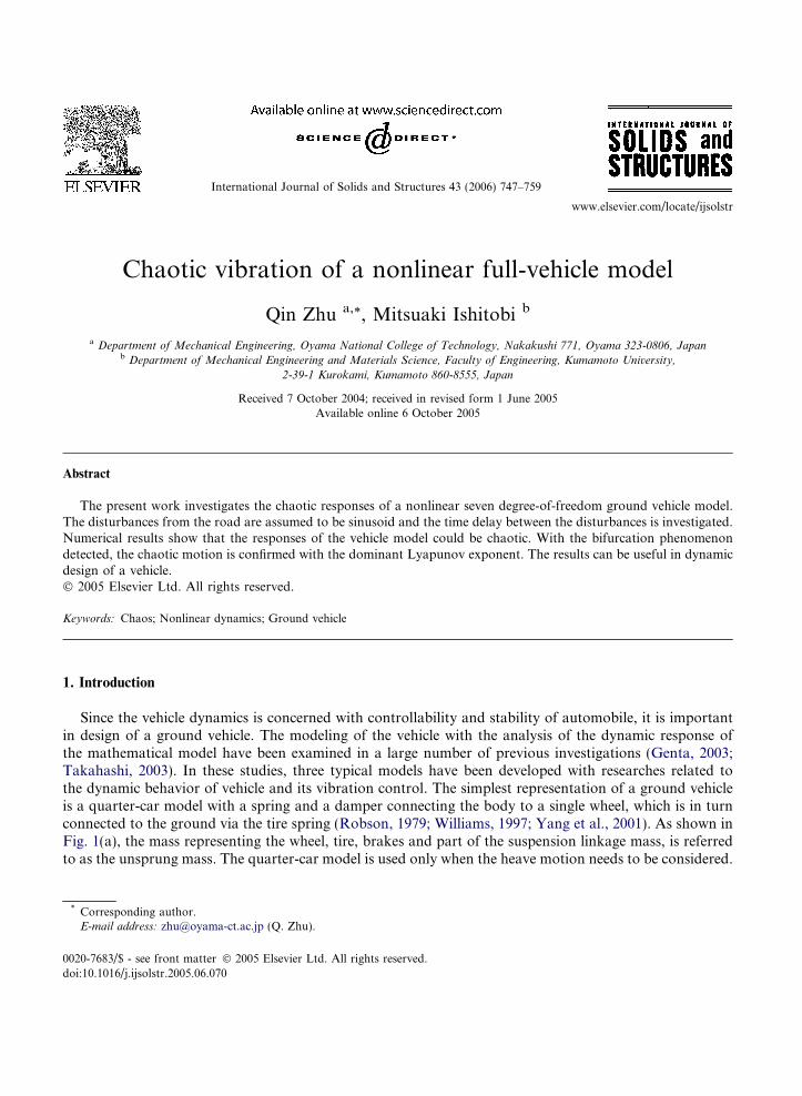
Since the vehicle dynamics is concerned with controllability and stability of automobile, it is importantin design of a ground vehicle. The modeling of the vehicle with the analysis of the dynamic response ofthe mathematical model have been examined in a large number of previous investigations (Genta, 2003;Takahashi, 2003). In these studies, three typical models have been developed with researches related tothe dynamic behavior of vehicle and its vibration control. The simplest representation of a ground vehicleis a quarter-car model with a spring and a damper connecting the body to a single wheel, which is in turnconnected to the ground via the tire spring (Robson, 1979; Williams, 1997; Yang et al., 2001). As shown inFig. 1(a), the mass representing the wheel, tire, brakes and part of the suspension linkage mass, is referredto as the unsprung mass. The quarter-car model is used only when the heave motion needs to be considered.

0020-7683/$ - see front matter � 2005 Elsevier Ltd. All rights reserved.doi:10.1016/j.ijsolstr.2005.06.070

* Corresponding author.E-mail address: [email protected] (Q. Zhu).

mailto:[email protected]

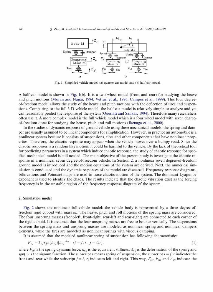
Fig. 1. Simplified vehicle model: (a) quarter-car model and (b) half-car model.

748 Q. Zhu, M. Ishitobi / International Journal of Solids and Structures 43 (2006) 747–759

A half-car model is shown in Fig. 1(b). It is a two wheel model (front and rear) for studying the heaveand pitch motions (Moran and Nagai, 1994; Vetturi et al., 1996; Campos et al., 1999). This four degree-of-freedom model allows the study of the heave and pitch motions with the deflection of tires and suspen-sions. Comparing to the full 3-D vehicle model, the half-car model is relatively simple to analyze and yetcan reasonably predict the response of the system (Oueslati and Sankar, 1994). Therefore many researchersoften use it. A more complex model is the full vehicle model which is a four wheel model with seven degree-of-freedom done for studying the heave, pitch and roll motions (Ikenaga et al., 2000).

In the studies of dynamic response of ground vehicle using these mechanical models, the spring and dam-per are usually assumed to be linear components for simplification. However, in practice an automobile is anonlinear system because it consists of suspensions, tires and other components that have nonlinear prop-erties. Therefore, the chaotic response may appear when the vehicle moves over a bumpy road. Since thechaotic responses is a random like motion, it could be harmful to the vehicle. By the lack of theoretical toolfor predicting parameters in a system which induce chaotic response, the study of chaotic response for spec-ified mechanical model is still needed. The main objective of the present study is investigate the chaotic re-sponse in a nonlinear seven degree-of-freedom vehicle. In Section 2, a nonlinear seven degree-of-freedomground model is introduced and the motion equations of the system are derived. Next, the numerical sim-ulation is conducted and the dynamic responses of the model are discussed. Frequency response diagrams,bifurcations and Poincare maps are used to trace chaotic motion of the system. The dominant Lyapunovexponent is used to identify the chaos. The results indicate that the chaotic vibration exist as the forcingfrequency is in the unstable region of the frequency response diagram of the system.

2. Simulation model

Fig. 2 shows the nonlinear full-vehicle model: the vehicle body is represented by a three degree-of-freedom rigid cuboid with mass ms. The heave, pitch and roll motions of the sprung mass are considered.The four unsprung masses (front-left, front-right, rear-left and rear-right) are connected to each corner ofthe rigid cuboid. It is assumed that the four unsprung masses are free to bounce vertically. The suspensionsbetween the sprung mass and unsprung masses are modeled as nonlinear spring and nonlinear damperselements, while the tires are modeled as nonlinear springs with viscous damping.

It is assumed that the modeled nonlinear spring of suspension has following characteristics:

F sij ¼ ksij sgnðDsijÞjDsijjnsij ði ¼ f ; r; j ¼ ‘; rÞ; ð1Þ
where Fsij is the spring dynamic force, ksij is the equivalent stiffness, Dsij is the deformation of the spring andsgn( Æ ) is the signum function. The subscript s means spring of suspension, the subscript i = f, r indicates thefront and rear while the subscript j = ‘, r, indicates left and right. This way, Fsfr, ksfr and Dsfr indicate the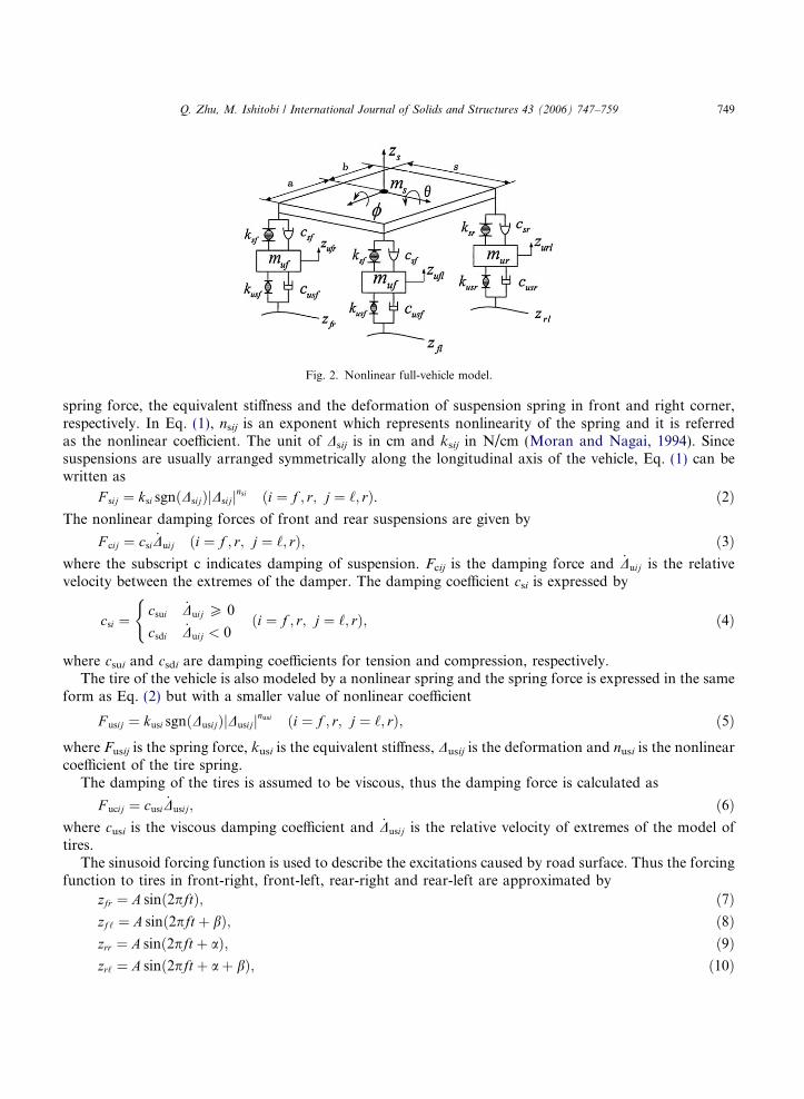

Fig. 2. Nonlinear full-vehicle model.

Q. Zhu, M. Ishitobi / International Journal of Solids and Structures 43 (2006) 747–759 749

spring force, the equivalent stiffness and the deformation of suspension spring in front and right corner,respectively. In Eq. (1), nsij is an exponent which represents nonlinearity of the spring and it is referredas the nonlinear coefficient. The unit of Dsij is in cm and ksij in N/cm (Moran and Nagai, 1994). Sincesuspensions are usually arranged symmetrically along the longitudinal axis of the vehicle, Eq. (1) can bewritten as

F sij ¼ ksi sgnðDsijÞjDsijjnsi ði ¼ f ; r; j ¼ ‘; rÞ. ð2Þ
The nonlinear damping forces of front and rear suspensions are given by
F cij ¼ csi _Duij ði ¼ f ; r; j ¼ ‘; rÞ; ð3Þ
where the subscript c indicates damping of suspension. Fcij is the damping force and _Duij is the relativevelocity between the extremes of the damper. The damping coefficient csi is expressed by
csi ¼csui _Duij P 0

csdi _Duij < 0

(ði ¼ f ; r; j ¼ ‘; rÞ; ð4Þ

where csui and csdi are damping coefficients for tension and compression, respectively.The tire of the vehicle is also modeled by a nonlinear spring and the spring force is expressed in the same

form as Eq. (2) but with a smaller value of nonlinear coefficient

F usij ¼ kusi sgnðDusijÞjDusijjnusi ði ¼ f ; r; j ¼ ‘; rÞ; ð5Þ
where Fusij is the spring force, kusi is the equivalent stiffness, Dusij is the deformation and nusi is the nonlinearcoefficient of the tire spring.
The damping of the tires is assumed to be viscous, thus the damping force is calculated as

F ucij ¼ cusi _Dusij; ð6Þ
where cusi is the viscous damping coefficient and _Dusij is the relative velocity of extremes of the model oftires.
The sinusoid forcing function is used to describe the excitations caused by road surface. Thus the forcingfunction to tires in front-right, front-left, rear-right and rear-left are approximated by

zfr ¼ A sinð2pftÞ; ð7Þzf ‘ ¼ A sinð2pft þ bÞ; ð8Þzrr ¼ A sinð2pft þ aÞ; ð9Þzr‘ ¼ A sinð2pft þ aþ bÞ; ð10Þ


where A and f are the amplitude and the frequency of the sinusoid road disturbance, respectively. Theparameter b indicates the time delay between the forcing functions to two front tires, or to two rear tires,respectively. On the other hand, a indicates the time delay between the forcing functions to front-right andrear-right tires ((7) and (9)) or to front-left and rear-left tires ((8) and (10)), respectively.

After applying a force-balance analysis to the model in Fig. 2, the equations of motion can be derived tothe static equilibrium positions.

Sprung mass:

ms€zs ¼ �F sf ‘ � F cf ‘ � F sfr � F cfr � F sr‘ � F cr‘ � F srr � F crr � msg; ð11Þ

I/€/ ¼�� F sf ‘ � F cf ‘ þ F sfr þ F cfr � F sr‘ � F cr‘ þ F srr þ F crr

� s2cos/; ð12Þ

Ih€h ¼�F sf ‘ þ F cf ‘ þ F sfr þ F cfr

�a cos h�

�F sr‘ þ F cr‘ þ F srr þ F crr

�b cos h. ð13Þ

Front unsprung masses:

muf€zuf ‘ ¼ F sf ‘ þ F cf ‘ � F usf ‘ � F ucf ‘ � muf g; ð14Þmuf€zufr ¼ F sfr þ F cfr � F usfr � F ucfr � muf g. ð15Þ

Rear unsprung masses:

mur€zur‘ ¼ F sr‘ þ F cr‘ � F usr‘ � F ucr‘ � murg; ð16Þmur€zurr ¼ F srr þ F crr � F usrr � F ucrr � murg. ð17Þ

The forces to the sprung mass in Eqs. (11)–(15) can be calculated as

F sf ‘ ¼ 100ðnsf�1Þksf sgnðDuf ‘ � Dsf ÞjDuf ‘ � Dsf jnsf ; ð18ÞF sfr ¼ 100ðnsf�1Þksf sgnðDufr � Dsf ÞjDufr � Dsf jnsf ; ð19ÞF cf ‘ ¼ csf _Duf ‘; ð20ÞF cfr ¼ csf _Dufr; ð21ÞF sr‘ ¼ 100ðnsr�1Þksr sgn Dur‘ � Dsrð Þ Dur‘ � Dsrj jnsr ; ð22ÞF srr ¼ 100ðnsr�1Þksr sgn Durr � Dsrð Þ Durr � Dsrj jnsr ; ð23ÞF cr‘ ¼ csr _Dur‘; ð24ÞF crr ¼ csr _Durr; ð25Þ

where

Duf ‘ ¼s2sin/� a sin hþ zs � zuf ‘; ð26Þ

Dufr ¼ � s2sin/� a sin hþ zs � zufr; ð27Þ

Dur‘ ¼s2sin/þ b sin hþ zs � zur‘; ð28Þ

Durr ¼ � s2sin/þ b sin hþ zs � zurr; ð29Þ

Dsr ¼a

100ðnsr�1Þksr

msg2ðaþ bÞ

� �� 1nsr

; ð30Þ

Dsf ¼b

100ðnsf�1Þksf

msg2ðaþ bÞ

� �" # 1nsf

. ð31Þ


The forces related to the unsprung mass in Eqs. (14)–(17) are expressed as

TableNumer

Param

SprungRoll axPitch aFrontRear uFrontRear sNonlinDampDampDampDampTire spDampNonlinLengthLengthWidth

F usf ‘ ¼ 100ðnf�1Þkusf sgnðDusf ‘ � Dsuf ÞjDusf ‘ � Dsuf jnusf ; ð32ÞF usfr ¼ 100ðnf�1Þkusf sgnðDusfr � Dsuf ÞjDusfr � Dsuf jnusf ; ð33ÞF ucf ‘ ¼ cusf _Dusf ‘; ð34ÞF ucfr ¼ cusf _Dusfr; ð35ÞF usr‘ ¼ 100ðnr�1Þkusr sgnðDusr‘ � DsurÞjDusr‘ � Dsurjnusr ; ð36ÞF usrr ¼ 100ðnr�1Þkusr sgnðDusrr � DsurÞjDusrr � Dsurjnusr ; ð37ÞF ucr‘ ¼ cusr _Dusr‘; ð38ÞF ucrr ¼ cusr _Dusrr, ð39Þ

where

Dusf ‘ ¼ zuf ‘ � A sinðxt þ bÞ; ð40ÞDusfr ¼ zufr � A sinðxtÞ; ð41ÞDusr‘ ¼ zur‘ � A sinðxt þ aþ bÞ; ð42ÞDusrr ¼ zurr � A sinðxt þ aÞ; ð43Þ

Dsur ¼g

100ðnr�1Þksur

msa2ðaþ bÞ þ mur

� �� 1nusr

; ð44Þ

Dsuf ¼ g

100ðnf�1Þksuf

msb2ðaþ bÞ þ muf

� �" # 1nusf

. ð45Þ

1ical values of the system parameters

eter Value

mass, ms 1500 kgis moment of inertia, I/ 460 kg mxis moment of inertia, Ih 2160 kg munsprung mass, muf 59 kgnsprung mass, mur 59 kgsuspension spring stiffness, ksf 35,000 N/muspension spring stiffness, ksr 38,000 N/mear coefficient of suspension spring, nsf, nsr 1.5ing coefficient of front suspension, csuf 1000 N/m/sing coefficient of front suspension, csdf 720 N/m/sing coefficient of rear suspension, csur 1000 N/m/sing coefficient of rear suspension, ccdr 720 N/m/sring stiffness, kusf, kusr 190,000 N/ming coefficient of tire, cusf, cusr 10 N/m/sear coefficient of tire spring, nusf, nusr 1.25between the front of vehicle and the center of gravity of sprung mass, a 1.4 mbetween the rear of vehicle and the center of gravity of sprung mass, b 1.7 mof sprung mass, s 3 m


Owing to the high nonlinearity of the suspension spring and damping forces, the system behaviordescribed by Eqs. (11)–(17) was studied numerically using the Runge–Kutta algorithm provided byMATLAB. In the computation, the absolute error tolerance was set to be lesser than 10�6. Since numericalintegration could give spurious results regarding the existence of chaos due to insufficient small time steps(Tongue, 1987), the step length was verified and it is ensure no such results were generated as a result oftime discretization. The frequency response diagram, Poincare maps and the dominant Lyapunov exponentwere used to identify the chaotic response. The parameters of the vehicle model which are used in thenumerical study are shown in Table 1.

3. Frequency response

In this section, the frequency response of the system is presented. The frequency response diagram,obtained by plotting the amplitude of the oscillating system versus the frequency of the excitation term,is often used to analyze the dynamics of a system (Belato et al., 2001). Since chaotic responses are pos-sible when the forcing frequency is within an unstable region, shown in frequency response diagram (Zhuet al., 1994; Pust and Szollos, 1999; Haller, 1997), then the forcing frequency for inducing chaos can bepredicted by studying unstable regions in the frequency response diagram. For the full-vehicle model, thefrequency response diagrams are plotted by defining the amplitude as the maximum absolute value of theamplitude of the displacement as in (Belato et al., 2001), and the frequency as frequency of the sinusoidroad disturbance. Fig. 3 represents the resonance curves of the heave, roll and pitch motion of sprungmass and heave motion of unsprung mass in front-left corner when the forcing frequency f is slowly in-creased and then slowly decreased. The diagrams were calculated by using an increment Df = 0.001 Hz asthe variation of the control parameter. The forcing frequency was in the range of 0.01 6 f 6 10 Hz. Thisparameter was changed 0.001 Hz with the time interval 50 s, so that the response diagrams can be pre-sumed to be continuous.

Fig. 3(a) and (b) show the frequency response diagram of the heave motion for the sprung mass.When the forcing frequency is increasing, there are three jumps at f = 3.51 Hz, f = 3.91 Hz andf = 4.82 Hz, while between f = 5.07 Hz and f = 5.39 Hz the oscillations change into beats. As shown inFig. 3(b), there are a small upward jump at f = 4.76 Hz and several small upward jumps aroundf = 2.92 Hz as the forcing frequency decreases. The beats begin at f = 5.39 Hz and end at f = 5.07 Hz.A new unstable region which does not exist as f is increasing appears in the forcing frequency2.92 < f < 3.34 Hz. Fig. 3(a) and (b) show that the numbers of jumps and unstable regions when forcingfrequency is increasing are different from ones as forcing frequency is decreasing. This phenomenon wasnot observed in study of dynamic responses of four degree-of-freedom nonlinear half-car model or twodegree-of-freedom nonlinear quarter-car model.

The frequency responses for roll motion of sprung mass are illustrated in Fig. 3(c) and (d). There is oneunstable region in 5.09 < f < 5.39 Hz when the frequency is increased. However, there are two unstable re-gions for decreasing frequency. One is in 5.07 < f < 5.39 Hz, another is in 2.93 < f < 3.55 Hz. Unlike theheave motion, there is only a small jump at 3.55 Hz for the decreasing frequency. Although the amplitudeof the response is small, the existence of unstable region and jumps indicate that chaos in roll motion mayexist.

The up and down jumps can be observed in frequency response diagram for the pitch motion of sprungmass shown in Fig. 3(e) as forcing frequency increases. There is one upward jump at f = 3.51 Hz, after-wards several downward jumps appear around f = 3.91 Hz. However, as shown in Fig. 3(f), there is onlyone upward jump at f = 3.55 Hz when forcing frequency decreases. Then, an unstable region with beatsfor pitch motion of sprung mass is in 5.09 < f < 5.40 Hz for both cases, when the forcing frequency is in-creased and decreased. Periodic responses also change to beating oscillations in 2.90 < f < 3.30 Hz when the

Fig. 3. Frequency response diagrams when the forcing frequency f is slowly increased and decreased (A = 0.06 m, b = 9�, a = 58�,0 < f < 10 Hz): (a) and (b) maxjzs(t)j; (c) and (d) maxj/(t)j; (e) and (f) maxjh(t)j; (g) and (h) maxjzuf‘(t)j.


frequency is decreasing. Therefore, there is one unstable region as the frequency is increased and two unsta-ble regions as the frequency is decreased.

Since the frequency response diagrams of the four unsprung masses have the same characteristics, onlythe frequency response diagram of one in front-left is plotted in Fig. 3(g) and (h). When the forcingfrequency is increased, one downward jump arises at f = 3.51 Hz. The periodic motion changes into beatsbetween f = 5.08 Hz and f = 5.40 Hz, which is surrounded by two regions with period-2 solutions. When


the forcing frequency is decreased, there are one upward jump at f = 3.55 Hz and several small upwardjumps around f = 2.92 Hz. Then there are two unstable regions, one is in 5.06 < f < 5.40 Hz and anotherin 2.93 < f < 3.34 Hz.

It is observed that the chaotic motion may not only appear as forcing frequency is within or near theunstable regions with beats, but also appear as forcing frequency is near one where the jump phenom-enon is observed. Therefore, the response diagrams of the studied model in Fig. 3 show that chaotic

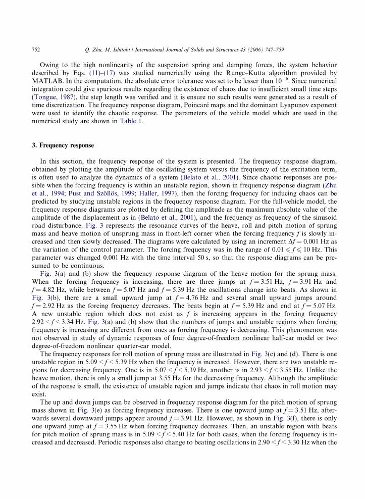
Fig. 4. Bifurcation diagrams obtained by varying a (A = 0.06 m, f = 3.2 Hz, b = 9�): (a) zs(t); (b) /(t); (c) h(t); (d) zuf‘(t); (e) zufr(t);(f) zur‘(t), and (g) zurr(t).


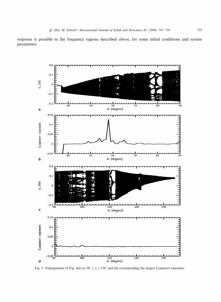
response is possible in the frequency regions described above, for some initial conditions and systemparameters.

Fig. 5. Enlargements of Fig. 4(a) as 34� 6 a 6 136� and the corresponding the largest Lyapunov exponent.

Fig. 6. Poincare maps of chaotic motion of the system (A = 0.06 m, f = 3.2 Hz, b = 9�, a = 58�).


Fig. 7. Time response of chaotic motion of zs(t) (A = 0.06 m, f = 3.2 Hz, b = 9�, a = 58�).



4. Bifurcation and chaos

In this section, the effect of the choice of the system parameters on the bifurcation structure are dis-cussed. One of signals of impending chaotic behavior in dynamics systems is a series of changes in the nat-ure of the periodic motions as some parameters are varied. The phenomenon of sudden change in themotion as a parameter is varied is called bifurcation (Moon, 1992). To make the bifurcation diagram, somemeasure of the motion is plotted as a function of a system parameter. In this paper, the bifurcation diagramis obtained by plotting the Poincare points of the displacement concerning to one of the parameters of thesystem.

To investigate the effect of time delay a to the appearance of chaotic response, the bifurcation diagramsin 0� 6 a < 360� were constructed via direct integration of the Eqs. (11)–(17). One of the results is shown inFig. 4. The bifurcation diagrams of the system were obtained by plotting the Poincare points of the re-sponse against the time delay a. The integration time was set to be 300 excitation cycles and only the last100 Poincare points were collected at each a. The parameters of excitation used in the computation wereA = 0.06 m, f = 3.2 Hz and b = 9� and the initial conditions were set to zeros.

Fig. 4 indicates that the chaotic responses are possible as 0� 6 a 6 20�, 38� 6 a 6 136� and290� 6 a < 360�. It also shows that the responses of sprung mass and unsprung masses become chaoticsimultaneously. An enlargement of the bifurcation diagram (Fig. 4(a), for 38� 6 a 6 136�) is shown inFig. 5(a) and (c), where periodic and chaotic motions were observed. The corresponding the largest Lyapu-nov exponent are shown in Fig. 5(b) and (d).

The Poincare maps of the responses of the system when a = 58� are shown in Fig. 6. Each Poincare mapcontains 10,000 sampling points and shows the existence of strange attractors. To determine whether thetime responses corresponding to Fig. 6 were chaotic, the Wolf�s algorithm (Wolf et al., 1985) was usedto calculate the dominant Lyapunov exponent. The time histories of the system from t = 200 s tot = 1700 s were used in the computation and the dominant Lyapunov exponents calculated werekzs ¼ 0:128, k/ = 0.001, kh = 0.013, kzuf ‘ ¼ 0:087, kzufr ¼ 0:043, kzur‘ ¼ 0:501 and kzurr ¼ 0:172 in the unitof bits/second. Fig. 7 shows the time response of zs(t). A direct look at the response suggests that the mo-tion the mass ms appears strange where the beats like motion appears randomly. These results indicatedthat the responses of the system were chaotic.

5. Conclusions

Chaotic responses and bifurcations of a nonlinear seven degree-of-freedom ground vehicle model whichis subjected to sinusoid disturbance with time delay are studied through numerical simulation. It is foundthat, in frequency response diagrams, the number of unstable regions as the forcing frequency is increasingdifferentiates from one as the forcing frequency is decreasing. This is typical phenomenon for nonlineardynamical systems, however the phenomenon was not observed in study of dynamic responses of two orfour degree-of-freedom vehicle model. The increase of unstable regions in frequency response diagramsimplies that there are more parameters for inducing chaotic motion because chaos usually appears asthe forcing frequency is inside the unstable regions.

The results of numerical simulation also show that the chaotic response may appear in the unstableregion of frequency response diagram. As there is variation of time delay in the road disturbances, theresponses of the system may become chaotic. This result also implies that the chaotic vibration of the sys-tem could be avoided by making the possible frequency of excitation far from the unstable region in fre-quency response diagram.


References

Belato, D., Weber, H.I., Balthazar, J.M., Mook, M.D.T., 2001. Chaotic vibration of a nonideal electro-mechanical system.International Journal of Solids and Structures 38, 1699–1706.

Campos, J., Davis, L., Lewis, F.L., Ikenaga, S., Scully, S., Evans, M., 1999. Active suspension control of ground vehicle heave andpitch motions. In: Proceedings of the 7th IEEE Mediterranean Control Conference on Control and Automation, Haifa, Israel.

Genta, G., 2003. Motor Vehicle Dynamics, second ed. World Scientific, Singapore.Haller, G., 1997. Chaos Near Resonance. Springer, New York.Ikenaga, S., Lewis, F.L., Campos, J., Davis, L., 2000. Active suspension control of ground vehicle based on a full-vehicle model. In:

Proceedings of American Control Conference, Chicago, USA.Moon, F.C., 1992. Chaotic and Fractal Dynamics. John Wiley & Sons Inc.Moran, A., Nagai, M., 1994. Optimal active control of nonlinear vehicle suspension using neural networks. JSME International

Journal, Series C 37, 707–718.Oueslati, F., Sankar, S., 1994. A class of semi-active suspension schemes for vehicle vibration control. Journal of Sound and Vibration

173, 391–411.Pust, L., Szollos, O., 1999. The forced chaotic and irregular oscillations of the nonlinear two degrees of freedom (2dof) system.

International Journal of Bifurcation and Chaos 9, 479–491.Robson, J.D., 1979. Road surface description and vehicle response. International Journal of Vehicle Design 9, 25–35.Takahashi, T., 2003. Modeling, analysis and control methods for improving vehicle dynamic behavior (overview). R&D Review of

Toyota CRDL 38, 1–9.Tongue, B.H., 1987. Characteristics of numerical simulations of chaotic system. ASME Journal of Applied Mechanics 54, 695–699.Vetturi, D., Gadola, M., Cambiaghi, D., Manzo, L., 1996. Semi-active strategies for racing car suspension control. SAE Technical

Papers, No. 962553, II Motorsports Engineering Conference and Exposition, Dearborn, USA.Williams, R.A., 1997. Automotive active suspensions, Part 1: Basic principles. Journal of Automobile Engineering, Part D 211,

415–426.Wolf, A., Swift, J.B., Swinney, H.L., Vastano, J.A., 1985. Determining lyapunov exponents from a time series. Physica D 16, 285–317.Yang, J., Suematsu, Y., Kang, Z., 2001. IEEE Transactions on Control Systems Technology 9, 295–317.Zhu, Q., Tani, J., Takagi, T., 1994. Chaotic vibrations of a magnetically levitated system with two degrees of freedom. Journal of

Technical Physics 35, 171–184.

Documents

1-s2.0-S0020768305003409-main.pdf