1

Probability & StatisticsLecture 1

Michael Partensky

2

Objectives

Learn how to measure chances. The first definition of the probability (P) Predicting P in some simple cases Practice, practice and practice

3Topics of Discussion (1)

The Laws of Chance… Are they possible? Gambling – it’s serious On the shoulders of Giants

Collecting the data Random experiments and events. Sample space, sample sets. Operations on sample sets. Frequencies of events

The first definition of probability (P) Axioms of probability Frequency interpretation of P General properties of P (derivation from Axioms).

4Topics of Discussion (2)

Random variables and distribution functions.Discrete and continuous variables. Examples.

Distribution function for discrete variables.

Continuous distributions.

5On the shoulders of Giants

Pierre de Fermat, French mathematician (1601-1655)

Blaise Pascal, Frenh mathematician and philospher (1623-1662)

Christiaan Huygens, Dutch astronomert, mathematician, physicist (1629-1695)

Jacob Bernoulli,Swiss mathematician(1654-1705)

6Not only only from their achievements, but also from errors …

D'Alembert argued, that if two coins are tossed, there are three possible cases, namely:(1) both heads, (2) both tails, (3) a head and a tail. So he concluded that the probability of  " a head and a tail " is 1/3. If he had figured that this probability has something to do with the experimental frequency of the occurrence of the event, he might have changed his mind after tossing two coins more than few times. Apparently, he never did do. Why? We do not know.

Was he right?

Think!

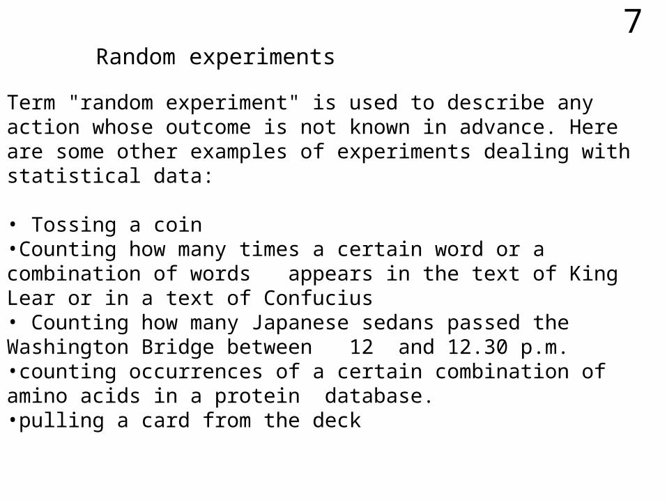
7Random experiments

Term "random experiment" is used to describe any action whose outcome is not known in advance. Here are some other examples of experiments dealing with statistical data:

• Tossing a coin •Counting how many times a certain word or a combination of words appears in the text of King Lear or in a text of Confucius • Counting how many Japanese sedans passed the Washington Bridge between 12 and 12.30 p.m. •counting occurrences of a certain combination of amino acids in a protein database. •pulling a card from the deck

8Sample spaces, sample sets and events

The sample space of a random experiment is a set that includes all possible outcomes of the experiment. For example, if the experiment is to throw a die and record the outcome, the sample space is = {1, 2, 3, 4, 5, 6}, the set of possible outcomes. describes an event that always occurs.

Certain subsets of the sample space of an experiment are referred to as events. An event is a set of outcomes of the experiment. Each time the experiment is run, a given event A either occurs, if the outcome of the experiment is an element of A, or does not occur, if the outcome of the experiment is not an element of A.

What to consider an event is decided by the experimentalist.

In any given experiment, there are always different ways to define an event. Please, illustrate this statement with examples.

9The examples of sample spaces and events

Example 1.1 Flip two coins. Try to figure out what is the sample space for this experiment How many simple events does it contain?

1 \ 2 H T

H HH HT

T TH TT

The answer could be described by a following table:

10The examples of sample spaces and events

Example 1.2Role two dice. For convenience we assume that one is red and the other is green(we often use this trick which hints that we can tell between two objects which is which. The following table describes

1 2 3 4 5 6

1 11 12 13 14 15 16

2 21 22 23 24 25 26

3 31 32 33 34 35 36

4 41 42 43 44 45 46

5 51 52 53 54 55 56

6 61 62 63 64 65 66

11Sample spaces and events

Example 1.2 (continued) . Any event corresponds to some collection of the cells of this table. We showed here three different events. Try to describe them in plain English

1 2 3 4 5 6

1 11 12 13 14 15 16

2 21 22 23 24 25 26

3 31 32 33 34 35 36

4 41 42 43 44 45 46

5 51 52 53 54 55 56

6 61 62 63 64 65 66

12Sample spaces and events

Example 1.2 (continued) . And what about the following events?Which of these event (red, orange, purple, etc) occurs more often?

1 2 3 4 5 6

1 11 12 13 14 15 16

2 21 22 23 24 25 26

3 31 32 33 34 35 36

4 41 42 43 44 45 46

5 51 52 53 54 55 56

6 61 62 63 64 65 66

13Sample spaces and events

Example 1.3 An experiment consists of drawing two numbered balls from the box of balls numbered from 1 to 9. Describe the sample space if

(a) The first ball is not replaced before the second is drawn.(b) The first ball is replaced before the second is drawn.

Example 1.4 Flip three coins. Show the sample space. What is the total number of all possible outcomes?

14

15

Composite eventsQuite often we are dealing with composite events. Example. We study a group of students, picking them at random and considering the following events: A = “A student is female”, B=“A student is male”, C= “A student has blue eyes”, D=“A student was born in California”.

After this information was collected and the probabilities of A. B, C and D were determined, we decided to find the probabilities of some other events:

U= “Student is female with blue eyes”, V=“Student is male, or has blue eyes and was not born in California”, etc. The latter questions are dealing with the events that are composed from the “atomic” events A, B, C and D. To describe them, it is convenient to use a language of the Set Theory.

Warning: please, don’t be scared. We are not going to be too theoretical. The new symbols will be introduced for our convenience.

16

ABInclusion: A is a subset of B

Occurrence of A implies the occurrence of B.Example: B = {2,3,5,6}, A={2,6}

AAB

B

Intersection: AB belongs to A and B Examples: (1) B = {2,3,4,6}, A={1,2,5,6} AB ={2,6}; (2) A=“Female students”, B=“Students having blue eyes”, AB = “Female students with blue eyes”.

17

ABA BThe union of events A and B, AB is the

event that A or B or both occur. Example: A = “Male student”, B= “Having blue eyes”, AB =“Students who are either male or have blue eyes (or both)”

B A

The empty set is the event with no outcomes. The events are disjoined if they do not have outcomes in common: A B= .

Example: A={1,3,4}, B= {2,4,6}

Operations on sample sets (1)

18

The first definition of probability

We introduced some important concepts:

Experiments, Outcomes, Sample space, Random variables.

These concepts will come to life after we introduce another crucial concept- probability, which is a way of measuring the chance.

A probability is a way of assigning numbers to events that satisfies following conditions or

19

The Axioms of Probability

(1) For any event A, 0P(A) 1. (1.1)(2) If is the sample space, then  P( )=1 (1.2)

(3) For a sequence of disjoined (incompatible) events Ai (finite or infinite), 1 3( ) ( ) ( . )i i i

i

P A P A

In other words, the probability for a set of disjoined events equals the sum of individual probabilities

We will introduce here another important property, although it is not an Axiom and will be justified later in the lecture devoted to the analysis of conditional probability:

20(4) If A and B are independent, then

1 4( ) ( ) ( ) ( . )P A B P A P B

In other words, for any number of independent events,

1 5( . )( )P A Ai i i

Incompatible (disjoined) and independent events

These new concepts introduced above require some explanation.

•Two events are said to be incompatible or disjoined if they can not occur together.

•Two events are said to be independent if they have “nothing to do” with each other.

21

Examples:

•Jack can arrive to Boston either on Monday (“M”) or on Wednesday (“W”). These events can not occur together (he can not arrive on Monday and on Wednesday). Therefore the events are disjoined. If P(M)=0.72 and P(W)=0.2, thenP(M or W)=0.92 (there is still a chance that Jack won’t come at all).

•You can get A or B with probabilities P(A) = 0.2 and P(B)=0.4.What is the probability of getting either A or B?

• A= “It will be sunny today”, B=“Celtic will win the game tomorrow”P(A and B)=P(A) P(B).

Please, offer some more examples of both kinds.

You can find a very useful and provocative discussion of these concepts and of the probability in general in the book “Chance and Chaos” by David Ruelle (Princeton Sci. Lib.)

22

Frequency interpretation of probability

If we repeat an experiment a large number of times, then

the fraction of times the event A occurs will be close to P(A).

In other words, if N(A,n) is the number of times that event occurs

in the first n trials, than

It's easy to prove that defined this way, P(A) satisfies conditions

(1) and (2) (Try to prove it).

Hint: the property (3) follows from

1 6( , )

( ) lim ( . )n

N A nP A

n

( , ) ( , )i i ii

N A n N A n

23Some other properties of probability. Deduction from the axioms 1-3:

1 71 81 9

c(a). Given that A +A we find from (3): c P(A)=1 - P(A ) ( . ).

(b) if A B, then P(A) ( ) ( . )(c) P(A ) ( ) ( ) ( ) ( . )

P BB P A P B P AB

A BAB

Try to prove (a) and (b). The property (c) is harder to prove formally, although intuitively it is quite clear. Summing up the areas of A and B, one counts their intersection twice. The probability is kind-a proportional to the area. Therefore, one of the occurrences of AB should be removed.

24

Random Variables and the Distribution Function.

The simplest experiments are flipping coins and throwing dice. Before we can say anything about the probabilities of their various outcomes (such as "Getting an even number" on the die, or "Getting 3 heads in 5 consecutive experiments with a coin") we need to make a reasonable guess about the probabilities of the elementary events (getting H or T for a coin , or one of six faces for a die). For instance, we can assume (as we usually do) that a die is perfectly balanced and all faces are equivalent. Then , the probability of any number equals 1/6.

As we will see, it can be described in terms of distribution (because it distributes probabilities between different outcomes) function.

The term “function”, however, implies some arguments (or variables). It would be inconvenient to use a “function of faces”, or a “functions of Heads or Tails”. That’s why we will introduce a general term for describing various random outcomes.

25

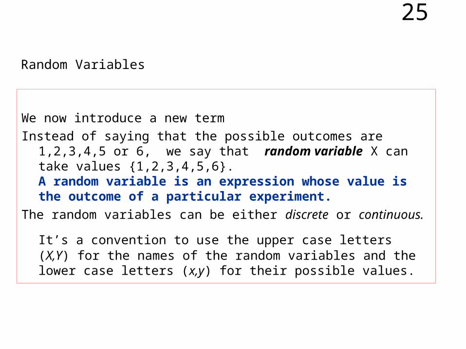
Random Variables

We now introduce a new term

Instead of saying that the possible outcomes are 1,2,3,4,5 or 6, we say that random variable X can take values {1,2,3,4,5,6}.A random variable is an expression whose value is the outcome of a particular experiment.

The random variables can be either discrete or continuous.

It’s a convention to use the upper case letters (X,Y) for the names of the random variables and the lower case letters (x,y) for their possible values.

26

Examples of random variables

Discrete: (you name !)

Continuous:

For instance, weights or a heights of people chosen randomly, amount of water or electricity used during a day, speed of cars passing an intersection.

Please, add a few more examples.

27

The Probability Function for discrete random variables We assigned a probability 1/6 to each face of the dice. In the same manner, we should assign a

probability 1/2 to the sides of a coin.

What we did could be described as distributing the values of probability between different elementary events:

P(X=xk)=p(xk), k=1,2,… (1.9)

It is convenient to introduce the probability function p(x) :P(X=x)=p(x) (1.10)

In other words, the probability of a random variable X taking a particular value xIs called the probability function.

For x=xk (1.10) reduces to (1.9) while for other values of x, p(x)=0.

28

The probability function should satisfy the following equations :

0 1 11

1 1 12

1 13

( ) ( . )

( ) ( . )

( ) ( ) ( . )

ii

ii E

p x

p x

P E p x

Example:

Suppose that a coin is tossed twice, so that the sample space is ={HH,HT,TH,TT}.

Let X represent a number of heads that can come up. Find the probability function p(x).

Assuming that the coin is fair, we have P(HH)=1/4, P(HT)=P(TH)=1/4, P(TT)=1/4;Then, P(X=0)=P(TT)=1/4; P(X=1)=P(HTTH)=1/4+1/4=1/2. P(X=2)= ¼.

29

The probability function is thus given by the table:

x 0 1 2

p(x) 1/4 1/2 1/4

The probability function p(x) is related to the probability density function (PDF) f(x) introduced in the next section for the continuous random variables. For those familiar with the concept of “-function”, this relation can be presented as

1 14( ) ( ) ( ) ( . )f x p x x xii

All others can simply ignore this formula.

30Uniform and non-uniform distributions.

If all the outcomes of an experiment are equally probable, the corresponding probability function is called uniform. If the contrary is true, the probability function is non-uniform.

Example On the face of a die with 6 dots, 5 dots are filled, so that only the central one is left. What is the probability function for this case? The value X=1 will occur in average 2 times more often than in the balanced die. As a result, p(1)=1/3, p(2)=p(3)=p(4)=p(5) = 1/6 .

Working in groups

TryIt Suppose we pick a letter at random from the word TENNESSEE. What is the sample space and what is the probability function for the outcomes? Challenge: For two dice experiment, find the probability function for X=“ Sum of two throws”.

31Continuous distribution (preliminary remarks)

1 1 5 1

1 5 2

( ) ( . . )

( ) ( ) ( . . )

ii

ii E

f x

P E f x

Suppose that the circle has a unit circumference (we simply use units in which 2 Pi R=1).

32Continuous distribution. Probability density function (PDF).

Suppose that every point on the circle is labeled by its distance x from some reference point x=0. The experiment consists of spinning the pointer and recording the label of the point at the tip of the pointer. Let X is the corresponding random variable. The sample space is the interval [0,1). Suppose that all values of X are equally possible. We wish to describe it in terms of probability. If it was a discrete variable (such as a dice), we would simply assign to every outcome a fixed value of probability to all outcomes.. p(xi)=const.

However, for a continuous variable we must assign to each outcome a probability p(x )=0. Otherwise, we would not be able to fulfill the requirement 1.12.

Something is obviously wrong!

33Continuous distribution and the probability density function

1 1 16

1 17

( ) ( . )

( ) ( ) ( . )E

f x

P E f x dx

Dealing with the infinitesimal numbers is a tricky business indeed. Those who studied calculus aware of this.

The analogs of Eqs. 1.12 and 1.13 for the continuous distributions would be

A random variable X is said to have a continuous distribution with density function f(x) if for all a b we have

1 15( ) ( ) ( . )b

a

P a X b f x dx

34

P(E) is a probability that X belongs to E.

a b

f(x)

Geometrically, P(a<X<b) is the area under the curve f(x) between a and b.

P(a<X<b)

35Examples:

1. The uniform distribution on (a,b):

We are picking a value at random from (a,b).1

01 18

,( ) ( . )

a x bb af xotherwise

By direct integration you can verify that (1.18) satisfies the condition (1.16). We can now find PDF which describes the experiment with the spinner in which case b-a=2

1 0 220

,( )

xf

otherwise

The probability that the arrow will stop in the rage between and + equals /2.

36

0

01 19

,( ) ( . )

xe xf x

otherwise

2. The exponential distribution

Those who know how to integrate can verify that (1.19) satisfies (1.16)

(the total area under the curve f(x) equals 1.

Note: In Matematica, the integral of a function f[x] (notice that […] rather than (…) is used) can be found as:

Integrate[f[x],{x,x1,x2}] , Shift+Enter.

Here x1 and x2 are the limits of integration.

37

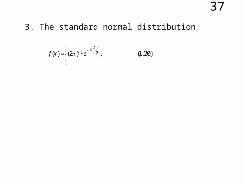
3. The standard normal distribution

21 22 1 20( ) ( ) , ( . )

xf x e

38