1

1. Overview

In these notes we discuss a family of linear analysis methods for identifying and documenting

preferred structures (i.e., linear relationships) in data sets that may be represented as two-

dimensional matrices.

1.1 Makeup of the input data matrix

The row and column indices of the input data matrix define the two domains of the analysis.

In general, the domains are some combination of parameter, space, and time1. ÔParameterÕ in

this discussion refers to scalar variables, such as geopotential height, temperature, zonal or

meridional wind components or ocean currents, concentrations of various chemical species,

satellite radiances in various wavelength bands, derived variables such as vorticity, diabatic

heating, etc. Space may be either one- two- or three-dimensional. By holding parameter, space or

time fixed, it is possible to generate three basic types of data input matrices:

(1) M x N matrices whose elements are values of a single parameter such as temperature at M

different spatial locations and N different times. Here the space domain is represented as a

vector, but the individual elements in that vector can be identified with a wide variety of two-or

three-dimensional spatial configurations: examples include regularly spaced gridpoint values or

irregularly spaced station values of the parameter at one or more levels, zonal averages of the

parameter at various latitudes and/or levels, and expansion coefficients of the basis functions of

a Fourier or EOF expansion of the field of the parameter. In most applications of this type a

row or column that represents the values of the parameter at a prescribed time can be represented

graphically; e.g., as a zonal, meridional or vertical profile; as a map; or as a vertical cross

section.

(2) M x N matrices whose elements are values of M different parameters measured at a single

fixed location in the space domain at N different times. The elements of a row (column) refer to

the values of the various parameters at a fixed time and the elements of the columns (rows) refer

to time series of a given parameter. Obviously, the matrix representation has a clear physical

interpretation only if the values of the parameters in a given row (or column) can be considered

to be simultaneous. This format might be used, for example, to study relationships in

measurements of a suite of pollutants and meteorological variables measured at a single urban

site.

(3) M x N matrices in which the M different parameters are defined a single point in the time

domain, but at N different locations. In this case, the elements of a particular column refer to

1 In some applications one of the domains may be identified with the "run number" in an ensemble of numerical

model integrations or monte carlo simulations.

2

values of the various parameters at a fixed location and the elements of a row refer to values of a

given parameter at various locations. All the parameters included in the analysis need to be

defined at the same set of locations.2

Linear matrix analysis techniques can also be applied to input data matrices that are hybrids of

the above types as illustrated in the following examples:

(a) One of the domains of the matrix may be a mix of space and time: e.g.suites of

measurements of P chemicals (or values of a single parameter P levels) at S different stations

and T different times may be arranged in an P x (S x T) matrix.

(b) Station or gridpoint representations of the spatial fields of P different parameters, each

defined at S locations and T times, may be arranged in a (P x S) x T matrix. In this manner, for

example, data for fields of the zonal and meridional wind components can be incorporated into

the same analysis.

The spacing of the data in the time and space domains need not be regular or in any prescribed

order so long as the parameter/space/time identification of the various rows and columns in the

input data matrix is preserved. For example, an analysis might be based upon daily or monthly

data for a number of different winter seasons. The analysis can be carried out in the presence of

missing elements in the input data matrix (see section 1.x). The impact of missing data upon the

results depends upon the fraction of the data that are missing and the statistical significance or

robustness of the structures inherent in the data.

1.2 Structure versus sampling

In most applications the structure of the input data matrix, that will hopefully be revealed by

the analysis and reproduced in analyses based on independent data sets, resides in one of the two

analysis domains and the sampling of that structure takes place in the other domain. The structures

that atmospheric scientists and oceanographers are interested in usually involve spatial patterns in

the distribution of a single parameter and/or linear relationships between different parameters.

Sampling usually involves realizations of those structures in the time domain (or sometimes in the

combined space/time domain). In some of the methods that will be discussed the distinction

between the Ôdomain of the samplingÕ and the Ôdomain of the structureÕ is obvious from the

makeup of the input data matrices but in others it is determined solely by the statistical context of

the analysis.

2 In the analysis of data from tree rings or sediment cores, the individual rings or varves in the sample are

identified with years in the reconstructed time series. Hence, one of the domains in the analysis may be interpreted

either as space (within the laboratory sample) or as the time in the historical record at which that ring or varve was

formed.

3

As in linear regression analysis, in order to obtain solutions, it is necessary that the effective

number of degrees of freedom in the domain of the sampling be as large or larger than the effective

number of degrees of freedom in the domain of the structure. In order to obtain statistically

significant (i.e., reproducible) results, it must be much larger. Geophysical data are characterized

by strong autocorrelation in the space and time domains. Hence, the effective number of degrees

of freedom may be much smaller than the dimension of the rows or columns in the data input

matrix. It follows that the Ôaspect ratioÕ M/N of the matrix may not be a good indicator of whether

the analysis is likely to yield statistically significant results: in some cases it may be overly

optimistic; in others it may be far roo pessimistic.

1.3 Analysis methods

Eigenvector analysis, commonly referred to as empirical orthogonal function (EOF) analysis in

the geophysical sciences literature after Lorenz (195x), is concerned with the structure of a single

input data matrix. Singular value decomposition (SVD) analysis and canonical correlation analysis

(CCA) are both concerned with linearly related structures in two different input data matrices, but

they use different criteria as a basis for defining the dominant structures. All three of these analysis

techniques can be performed using a single fundamental matrix operation: singular value

decomposition. Henceforth in these notes the term Ôsingular value decompositionÕ (as opposed to

ÔSVD analysisÕ) will be used to refer to this operation, irrespective of whether it is being performed

for the purpose of EOF analysis, SVD analysis or CCA. EOF analysis can also be performed

using matrix diagonalization instead of singular value decomposition.

1.4 Format of the results

The methods described here all yield a finite number of modes. Each mode in an EOF analysis

is identified by an eigenvalue (a positive definite number which defines its rank and relative

importance in the hierarchy of modes), an eigenvector or EOF (a linear combination of the input

variables in the domain of the structure), and a principal component (PC) which documents the

amplitude and polarity of that structure in the domain of the sampling. In the terminology of

Fourier analysis, the PCÕs are the expansion coefficients of the EOFÕs. Each mode in SVD

analysis is defined by a singular value (a positive definite number which defines its rank and

relative importance in the hierarchy of modes), and a pair of structures, referred to as singular

vectors, each with its own set of expansion coefficients that document its variability in the

domain of the sampling. The corresponding quantities in CCA are referred to as canonical

correlations, canonical correlation vectors, and expansion coefficients. In general, the number

of modes obtained from these analysis techniques is equal to the number of rows or columns of the

4

input data matrix (the smaller of the two). However, in most applications, only the leading mode

or modes are of interest in their own right.

1.5 Applications of EOF analysis

(a) data compression

Geophysical data sets for spatial fields are sometimes transformed into time series of expansion

coefficients of sets of orthonormal spatial functions for purposes of archival and transmission.

The most common example is the use of spherical harmonics (products of Legendre functions in

latitude and paired, quantized sine/cosine functions in longitude) for data sets generated by

numerical weather prediction models. Since most of the variance of atmospheric variables tends to

be concentrated in the leading modes in such representations, it is often possible to represent the

features of interest with a truncated set of spectral coefficients. The more severe the truncation the

greater compression of the data. Of all space/time expansions of this type, EOF analysis is, by

construction, the most efficient: i.e., it is the method that is capable of accounting for the largest

possible fraction of the temporal variance of the field with a given number of expansion

coefficients. For some investigators, EOF analysis may also have the advantage of being the most

accessible data compression method, since it is offered as a standard part of many matrix

manipulation and statistical program packages.

For certain applications, the efficiency of EOF analysis in representing seemingly complex

patterns is nothing short of spectacular: a classic example is the human fingerprint, which can be

represented in remarkable detail by the superposition of fewer than ten EOF's. On the other hand,

it will be shown in section 2.7 that EOF analysis is no more efficient at representing "red noise" in

the space domain than conventional Fourier expansions. In general EOF analysis is more likely to

excel, in comparison to Fourier expansions, when the field to be expanded is simple in ways that

conventional Fourier analysis is unable to exploit. For example, the fingerprint pattern is not as

complicated as its fine structure would imply: the features of interest are made up of quasi-periodic

elements with a narrow range of two-dimensional wavenumbers (in x,y). A conventional Fourier

description would require carrying along a great deal of excess baggage associated with lower

wavenumbers (larger space scales), which would be of little interest in this particular case even if

they were present. Geophysical analogues to the fingerprint pattern might include homogeneous

fields of ocean waves, sand dunes, or cellular convection in a stratus cloud deck. EOF expansions

are likely to be less efficient when the fields are nonhomogeneous; e.g., when the edge of a cloud

deck cuts across the image.

In general, fields that are highly anisotropic, highly structured, local in either the space domain

or in the wavenumber domain are likely to be efficiently represented by EOFÕs and their associated

5

PCÕs. Recurrent spatial patterns of this type are likely to be associated with boundary conditions

such as topographical features or coastlines, or with certain types of hydrodynamic instabilities.

Even in situations in which EOF analysis is demonstrably the most efficient representation of a

dataset, the conventional Fourier representation is still usually preferred by virtue of its

uniqueness, its familiarity, and its precise and compact mathematical definition. In addition, the

transformation to Fourier coefficients may be substantially more efficient, in terms of computer

resources, than a transformation to PCÕs in the case of large arrays. In many numerical models

the Fourier coefficients are used, not only for representing the fields, but also as a framework for

representing the governing equations and carrying out the calculations.

(b) pre-filtering

In types of linear analysis procedures such as multiple regression and canonical correlation

analysis it is convenient to preprocess that data to obtain sets of input time series that are mutually

orthogonal in the time domain. This procedure simplifies the formalism, speeds up the calculations

and reduces the risk of computational problems. In addition, it offers the possibility of reducing

the number of input variables simply by truncating the PC expansion at some point, thereby

reducing computational and storage requirements. For certain kinds of calculations such as CCA,

such ÔprefilteringÕ is not only desirable, but may be absolutely necessary in order to ensure the

statistical reliability of the subsequent calculations. The optimality of EOF analysis in representing

as much as possible of the variance of the original time series in as few as possible mutual

orthogonal PCÕs renders it particularly attractive as a prefiltering algorithm. Although slightly less

efficient in this respect, rotated EOF analysis, which will be discussed in section 2.8, can also

serve as a prefiltering operation that yields mutually orthogonal expansion coefficient time series

for input to subsequent analysis schemes.

(c) exploratory analysis

When confronted with a new and unfamiliar dataset consisting of multiple samples of a spatial

field or a set of physical parameters, EOF analysis is one of the best ways of identifying what

spatial patterns (or linear combinations of physical parameters) may be present. If the patterns

revealed by the leading EOFÕs are merely a reflection of seasonal or diurnal variations in the data,

that should be clear from an inspection of the corresponding PCÕs. If they are associated with

boundary conditions or instabilities, the information on their shapes and time dependent behavior

provided by the EOFÕs and PCÕs may be helpful in identifying the processes involved in forcing or

generating them.

Because they are products of spatial patterns and time series, EOF/PC combinations are well

6

suited for resolving structures of the form y (x,t) = Y(x)coswt . Such structures are often

referred to as standing oscillations because their time evolution involves changes in the amplitude

and polarity of a pattern with geographically fixed nodes and antinodes. Normal mode solutions

are of the more general form y (x,t) = A(x)coswt + B(x)sinwt in which two different spatial

patterns appear in quadrature with one another in the time domain. A common pattern of this form

is a propagating wave in which A and B are of sinusoidal form in space and in quadrature with one

another. Such a pattern will typically be represented by a pair of EOF's whose time series will

oscillate in quadrature with one another, in conformity with the orthogonality constraint. In the

case of a pure propagating wave in a domain whose size is an integral multiple of the wavelength,

the eigenvalues corresponding to the two EOF patterns should be equal, indicating that any linear

combination of the two modes (i.e., any phase of the wave in the space domain) explains as much

variance as any other. However, as discussed in section 2.6, similar types of patterns are

observed in association with red noise. Therefore, in order to distinguish between propagating

waves and noise, it is necessary to examine the corresponding PC time series for evidence of a

quadrature phase relationship.

EOFÕs need not be associated with spatial patterns. Preferred linear combinations of physical

or chemical parameters may be associated with specific processes, sources or sinks, or forcing.

For example sunlight may enhance the concentrations of certain chemical tracers and decrease the

concentrations of others: a specific source of pollutants like a coal fired powerplant might be

recognizable as a certain linear combination of chemical species.

1.6 Applications of SVD analysis and CCA

In contrast to EOF analysis, which is concerned with the linear relationships that exist within a

single input data matrix, SVD analysis and CCA are concerned with the linear relationships

between the the variables in two different input data matrices, which share a common Ôdomain of

the samplingÕ. To illustrate with an example from psychology, the domain of the sampling might

be the individual subjects who filled out a pair of questionnaires: one concerned with personality

traits and the other with job preferences. The data from the two questionnaires could be pooled in

a single EOF analysis that would attempt to identify preferred linear combinations in the responses

to the combined set of questions. Alternatively, preferred linear combinations of the responses to

the questions on the personality questionnaire could be related to linear combinations of the

responses to the questions on the job preference questionnaire using SVD analysis or CCA. The

resulting ÔmodesÕ would identify patterns in personality traits that could be used to infer or predict

how individuals would respond to the questions about job preferences (e.g., people who are

extroverts are more inclined towards sales and management jobs).

7

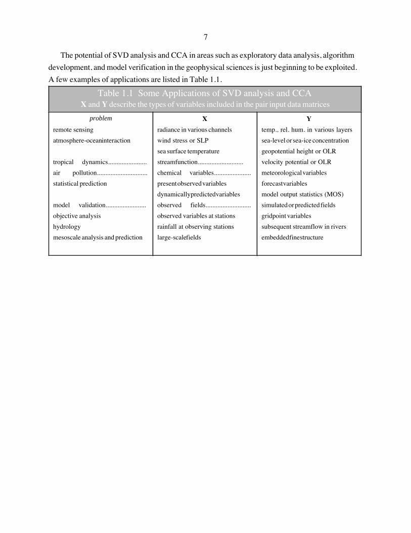
The potential of SVD analysis and CCA in areas such as exploratory data analysis, algorithm

development, and model verification in the geophysical sciences is just beginning to be exploited.

A few examples of applications are listed in Table 1.1.

Table 1.1 Some Applications of SVD analysis and CCAX and Y describe the types of variables included in the pair input data matrices

problem

remote sensing

atmosphere-ocean interaction

tropical dynamics.......................

air pollution..............................

statistical prediction

model validation........................

objective analysis

hydrology

mesoscale analysis and prediction

X

radiance in various channels

wind stress or SLP

sea surface temperature

streamfunction...........................

chemical variables......................

present observed variables

dynamically predicted variables

observed fields...........................

observed variables at stations

rainfall at observing stations

large-scale fields

Y

temp., rel. hum. in various layers

sea-level or sea-ice concentration

geopotential height or OLR

velocity potential or OLR

meteorological variables

forecast variables

model output statistics (MOS)

simulated or predicted fields

gridpoint variables

subsequent streamflow in rivers

embedded fine structure

8

2. EOF Analysis

2.1 Introduction and general formalism

Empirical orthogonal function (EOF) analysis (sometimes also referred to as Principal

Component analysis (PCA)) may be performed by diagonalizing the dispersion matrix C to obtain

a mutually orthogonal set of patterns comprising the matrix E, analogous to the mathematical

functions derived from Fourier analysis, and a corresponding expansion coefficient matrix Z,

whose columns are mutually orthogonal. The patterns are called EOFÕs (or eigenvectors) and the

expansion coefficients as referred to as the the principal components (PCÕs) of the input data

matrix. The leading EOF e1 is the linear combination of the input variables xj that explains the

largest possible fraction of the combined dispersion of the XÕs: the second e2 is the linear

combination that explains the largest possible fraction of the residual dispersion, and so on.

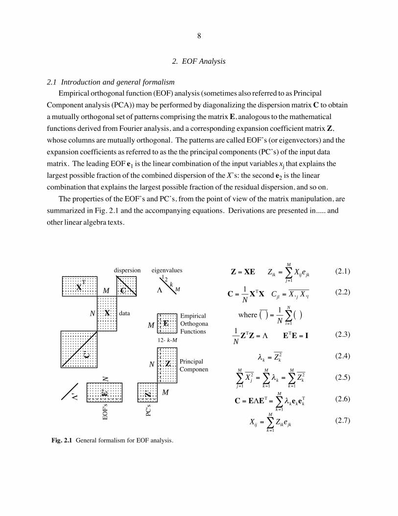
The properties of the EOFÕs and PCÕs, from the point of view of the matrix manipulation, are

summarized in Fig. 2.1 and the accompanying equations. Derivations are presented in..... and

other linear algebra texts.

M

N

X

E

C

C'

X

dispersion

Empirical OrthogonalFunctions

Principal Component

MLk

eigenvalues12

N

M

12- k-M

Z

T

M

EO

F's

E'

L' Z'

PC's

N

data

Fig. 2.1 General formalism for EOF analysis.

Z XE= Z X eik ij jkj

M

==

å1

C =1NXTX

Cjl = X. j X.l

where

( ) =1N

( )i =1

N

å

1NZTZ = L ETE = I

l k = Zk

2

Xj2

j =1

M

å = l kk=1

M

å = Zk2

k=1

M

å

C = ELET

= l kk=1

M

å ekekT

Xij = Zikk=1

M

å ejk

(2.1)

(2.2)

(2.3)

(2.4)

(2.5)

(2.6)

(2.7)

9

The subscript ( )i

is a row index wherever it appears and ( )k

is a column index associated with

the individual EOF/PC modes. ( ) j

is the column index in X and the row index in E and Z. M is

the smaller dimension of the input data matrix X and N is the larger dimension. Capital X’s (lower

case x’s) refer to input data from which the column means have not (have) been removed.

Equation (2.1) identifies the EOFÕs as linear combinations of the input variables (XÕs) that

transform them into PCÕs (ZÕs). Eq. (2.2) defines the dispersion matrix C, which is the input to

the matrix diagonalization routine which yields the eigenvalues (lk) and EOFÕs (ek). Eq. (2.3)

specifies that both the EOFÕs and PCÕs are mutually orthogonal: the EOFÕs are of unit length and

the lengths of the PCÕs are equal to the square roots of their respective eigenvalues. The

relationship between the squared length (or dispersion) of the PCÕs and the eigenvalues is

expressed in component form in (2.4). Eq. (2.5) shows that the total dispersion of the input

variables is conserved when they are transformed into PCÕs. From (2.4) and (2.5) it is evident that

that the dispersion of the XÕs is apportioned among the various PCÕs in proportion to their

respective eigenvalues. Eq. 2.6 shows how the dispersion matrix can be reconstructed from the

eigenvectors and eigenvalues. Each mode can be seen as contributing to each element in the

matrix. Eq. 2.7 shows how the input data can be represented as a sum of the contributions of the

various EOF modes, each weighted by the corresponding PC, much as a continuous field can be

represented as a sum of the contributions of functions derived from a Fourier expansion, each

weighted by the corresponding expansion coefficient.

Either of the dispersion matrices C and CÕ can be formed in three different ways: (1) as the

product matrix X·j X·l , in which the means

X·j are not necessarily equal to zero; (2) as the

covariance matrix x·j x·l , or (3) as the correlation matrix3

r x·j ,x·l( ). The diagonal elements of

the covariance matrix are the variances and the trace is equal to the total variance. The diagonal

elements of the correlation matrix are all equal to unity, so that

l kk=1

M

å = M . Regardless of how it is

formed, the dispersion matrix is symmetric, i.e., Cjl = Clj .

If the columns (rows) of the input data matrix X have zero mean, the diagonal elements of the

dispersion matrix C (CÕ) will correspond to variances and the principal components corresponding

to each EOF mode will have zero mean. If the rows (columns) of X have zero mean, the eigen-

vectors ek. (

¢ek) will have zero mean. Further discussion of how removing (or not removing) the

means from the input data matrix affects the results of EOF analysis is deferred to the next section.

3 A convenient way to form the correlation matrix, based on the product moment formula, is to divide all theelements in each row of the covariance matrix by the standard deviation for that row, which is simply the square rootof the diagonal element for that row, and then divide all the elements in each column by the standard deviation forthat column.

10

2.1.1 EOF analysis by singular value decomposition of the input data matrix

As an alternative to diagonalizing C or CÕ, it is possible to obtain the eigenvalue, EOF and PC

matrices as products of singular value decomposition of the input data matrix X:

X = ULV xij = l kk=1,Må uikvjk = l k

k=1,Må vikujk

In practice, this method of calculation is often the most convenient in the sense that it requires

the minimal amount of customized programming, and it may prove to be the most efficient in terms

of computer time. The only cases in which diagonalizing the dispersion matrix may be the method

of choice are those in which the input matrix is large enough to be of concern in terms of memory

requirements, and/or N>>M.

2.1.2 EOF’s versus PC’s: a statistical perspective

As shown in Fig. 2.1, dispersion matrices can be formed by averaging over either the rows or

the columns of X. Regardless of the way C is formed, the number of nonzero eigenvalues

obtained by diagonalizing it is less than or equal to the smaller dimension of X (M in Fig. 2.1).

Provided that the dispersion matrices are formed and the EOF and PC matrices are handled in a

consistent manner with respect to the removal of the row and column means, it can be shown that

l = ¢l

E = ¢Z and Z = ¢E (2.8)

Hence, the EOF and PC matrices are completely interchangeable from the point of view of the

matrix manipulation: one analystÕs EOFÕs may be another analystÕs PCÕs if one goes by the strictly

mathematical definition.4 This interchangeability is obvious if the EOFÕs and PCÕs are obtained

by singular value decomposition of the input data matrix, but it is no less valid if the EOFÕs are

obtained by diagonalizing either of the dispersion matrices.

However, as noted in section 1.2, the distinction between the EOFÕs and PCÕs is usually clear

in the statistical context of the analysis. The statistical significance or reproducibility of the

analysis resides in the EOFÕs: i.e., if the analysis were to be performed again, but on an

independent data set, it is the EOFÕs that would hopefully be reproducible in the new data set, not

the PCÕs, which are merely documenting the amplitiudes and polarities of the patterns in the

domain of the sampling. In most geophysical applications involving the input data defined in the

space/time or parameter/time domains, the EOFÕs correspond to spatial patterns or sets of relative

weights or loadings to be assigned to the various parameters included in the analysis, and the PCÕs

are time series that document the amplitude and polarity of the spatial patterns or weights during

some particular time interval. If the analysis is repeated on independent data, ÔindependentÕ usually

4 When the EOF and PC matrices are obtained by singular value decomposition of X, it is the analystsÕs choice

of which one is which.

11

refers a different period of record in the time domain. One hopes that the ÔpatternsÕ in physical

space or parameter space will not change radically from one (temporal) sample to another, but one

harbors no such hopes or expectations with respect to the time variability of the PCÕs. (In fact, if

the EOFÕs and PCÕs are both similar in two data sets, the data sets cannot be viewed as

independent samples.) Hence, in most applications the temporal dispersion matrix, in which the

overbar in (2.2), (2.4) and (2.5) refers to a time average, can be viewed as the essential input to the

EOF analysis upon which considerations of statistical significance should be based; the EOFÕs

define specific linear combinations of the input time series; and the PCÕs are the numerical values

of these linear combinations at each time at which the input data are sampled. The PCÕs may be

viewed as linear combinations of the input time series, as in (2.1), or (in the terminology of

Fourier analysis) as the expansion coefficients of the EOFÕs. These labels are applicable regardless

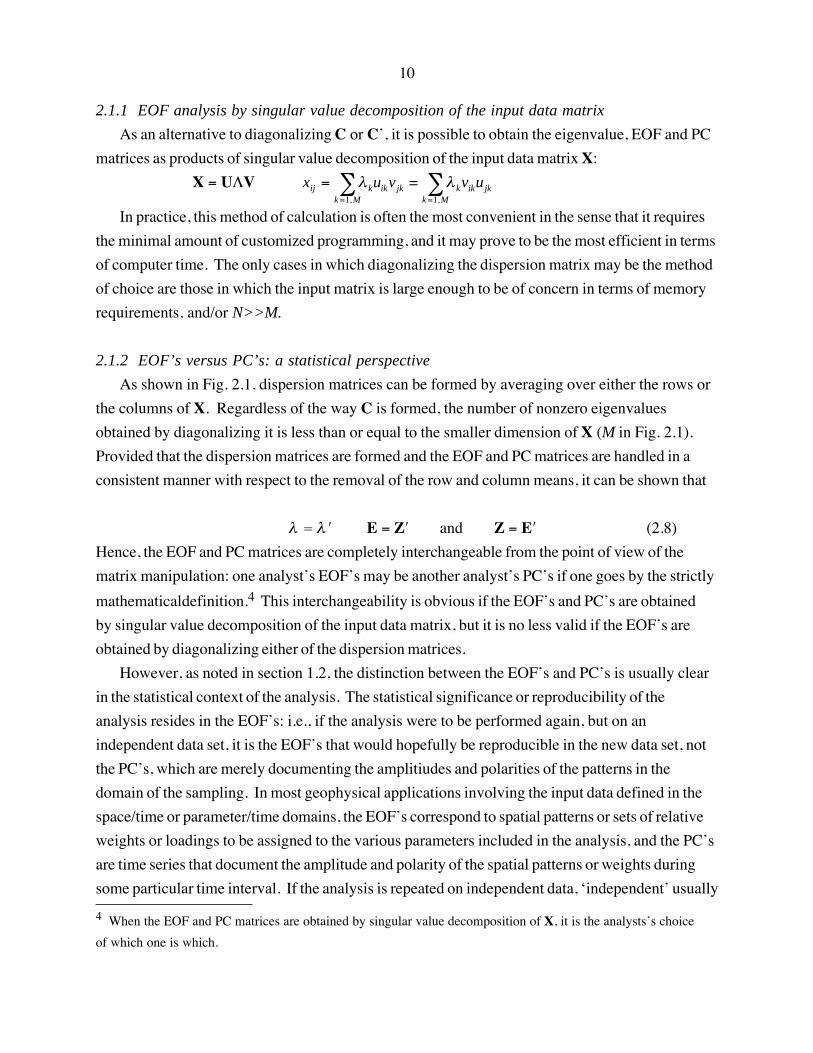
of how the calculations are performed.5 Henceforth, in these notes the spatial patterns (or

relative weights or loadings of the input parameters) will be referred to as EOFÕs and the

corresponding expansion coefficient time series as PCÕs, as indicated in Fig. 2.2. The subscript i

will be used as the row index in the domain of the sampling which can be assumed to be time

unless otherwise noted, j as a column index denoting parameter or position in space, and k as a

column index to denoting mode number. This notation is consistent with what has been used up to

this point, but it is more specific.

M

NE

C

X

dispersion

Empirical OrthogonalFunctions

Principal Components

MLk

eigenvalues12

N

M

12- k-M

Z

M

data

Fig. 2.2 Formalism for EOF analysis based on sampling in the time domain. Columns in the X and Z matrices

refer to time series, and columns in E to patterns. Rows in X refer to stations, gridpoints or physical parameters,

and rows in E and Z to EOF modes.

5 In interpreting the literature, it should not be assumed that all authors adhere to these labeling conventions.

12

2.1.3 A state space interpretation

The ith row in the input data matrix defines a single point in N dimensional space in which Xij

is the position along the jth coordinate. Each point constitutes a single realization of the input

variables. X in its entirety defines a cloud of points in that multidimensional Ôstate spaceÕ. The

EOFÕs define an orthogonal rotation of the state space, and the PCÕs define the positions of the data

points in the rotated coordinate system. The dispersion of the points along the axis of the leading

PC is maximized.

2.2 The input data matrix

With the statistically motivated definition of EOFÕs and PCÕs, the consequences of removing or

not removing the space and time means from the input data (or in the process of computing the

dispersion matrix becomes more clear. In many geophysical applications, time (column) means6

are removed from X, but not space (row) means. The dispersion matrix C is then equal to the

temporal variance matrix x·j x·l and the EOFÕs may be interpreted as orthogonal axes passing

through the centroid of the dataset in multi-dimensional phase space. Since the PC axes pass

through this same centroid, their time series also have zero mean. However, the components of

the individual EOFÕs in the space domain need not sum to zero. For example, one of the EOFÕs

could conceivably describe fluctuations that occur in phase in all the input time series, in which

case all the components of that mode would be of the same polarity.

In some instances it may be desirable to remove the means from the individual rows of X

before calculating the EOFÕs. For example, suppose that the columns of X are time series of

temperature at an evenly spaced array of gridpoints in a global domain. If one were interested, not

so much in the temperature itself, but in spatial temperature gradients that are coupled to the wind

field through the thermal wind equation, it might be advisable to analyze departures from global

mean temperature, rather than temperature itself. It is also possible that because of instrument

problems, measurements of temperature might be much less reliable than measurements of

temperature gradients. One might even consider going a step farther and removing, not only the

global mean, but also the zonal mean on each latitude, thereby isolating what is commonly referred

to as the ÔeddyÕ component of the field. Alternatively (or in addition), one could spatially smooth

the field in order to emphasize the larger scales; or remove a spatially smoothed version of the field

6 When removing the time mean from input data spanning several months or longer, the climatological mean

annual cycle may need to be considered. If one removes only the time mean from the input time series, the annual

march will contribute to the variance, and it will influence and perhaps even dominate the leading EOFÕs. Unless

one is specifically interested in the annual cycle, it is advisable to remove the first two or three harmonics of the

annual cycle from the input data matrix before performing the EOF analysis. Such an analysis is said to be

performed upon the anomalies of the field in question.

13

in order to isolate the variance associated with the smaller scales.

If the time means are not removed from the input data, products of time mean terms of the form

Xj

Xl will contribute to the elements of the dispersion matrix, so the dispersion and the eigenvalues

will be larger. Instead of passing through the centroid of the dataset in multi-dimensional phase

space the axes of the PCÕs pass through the origin. If the time means of the Xj Õs are large in

comparison to the variability about them, the leading EOF will be dominated by the mean field

(i.e., the PC axis directed from the origin toward the centroid of the dataset and the time mean of

the corresponding PC is likely to be large in comparison to its own standard deviation. Such

ÔnoncenteredÕ EOF expansions can be justified if the ratios of the various input variables (the X•j Õs)

are more likely to be useful as a basis for identifying patterns than ratios of the corresponding

departures from the means (the x•j Õs). Such expansions have been used in the analysis of sediment

records and they could conceivably be useful in the analysis of time series of chemical species or

meteorological fields such as precipitation, cloudiness, or wind speed which are positive definite

and may have highly skewed frequency distributions. For variables such as temperature or

geopotential height, the origin in phase space holds no special significance, but the departure from

a domain averaged or zonally averaged value might be be considered as input data for EOF analysis

(as opposed to departures from time means).

Normalizing the input data matrix is equivalent to replacing the dispersion or variance matrix by

the correlation matrix. If the input data were, for example, time series of chemical measurements

with widely differing amplitudes and perhaps even different units (ppm, ppb.A.), one would have

little choice but to normalize. Otherwise, the time series with the largest numerical values of

variance would be likely to determine the character of the leading EOFÕs. But when one is

analyzing a field such as 500 mb height, the choice of whether to normalize or not involves more

subtle considerations.

In general, the leading EOFÕs of unnormalized data explain more of the variance in the dataset

than their counterparts based on the correlation matrix and they tend to be statistically somewhat

more robust. The Ôcenters of actionÕ of the first few EOFÕs tend to be shifted towards and/or more

concentrated in the regions of high variance. Since the spatial gradients of the variance field are

inextricably linked to the spatial structure of the field, it seems artificial to eliminate them.

However, if one is interested in the strucure of the variability even in the relatively quiescent

regions of the field, EOFÕs based on the correlation matrix might provide some useful insights.

Under certain circumstances it may be advantageous to apply certain kinds of weighting to the

various variables xj that enter into the EOF analysis. For example, one might want to weight the

variance for each station by the geographical area that it represents. For a regular latitude-longitude

grid, this could be accomplished by multiplying each gridpoint value by the square root of cosine

14

of latitude. If data for two or more different fields, each with its own units are included in the

analysis (e.g., gridded data for pressure and temperature), it might be advisable to partition the

total variance among the fields intentionally, rather than leaving it to chance. In this case one

proceeds by (1) deciding what fraction of the total variance to assign to each field (e.g., one might

wish to divide it into equal parts so that each field gets equal weight in the analysis) (2) calculating

the variance that each field contributes to the total variance of the unweighted data, and (3)

weighting each input variable by the fraction of the total variance that one wishes to assign to its

field divided by that fieldÕs fractional contribution to the total variance of the unweighted data (both

square rooted). The weighting can be applied to the input data matrix directly, but it is often more

convenient to apply it to the rows and columns of the dispersion matrix.

2.2.1 Treatment of missing data

to be added

2.3 The dispersion matrix

The dispersion matrix contains information that may be of interest in its own right and it may

be of use in interpreting the EOFÕs. In most meteorological applications the means have been

removed from the input time series, so that the elements in this matrix are simply temporal

variances and covariances of the input variables. If, in addition, the input time series have been

normalized to unit variance, it is readily verified that the diagonal elements of the dispersion matrix

will all be equal to unity and the off diagonal elements to correlation coefficients. In this case it is

often referred to as the correlation matrix.

It is often informative to tabulate or map the diagonal elements of the covariance matrixwhich

represent the variances that will be reapportioned among the EOFÕs. The leading EOFÕs usually

tend to be dominated by the series that exhibit the largest variance.

2.4 The eigenvalues

The eigenvalues are all positive semidefinite and have units of dispersion (X squared). They

are ranked from largest (identified with the first or leading mode) to the smallest (the Mth)7.

Their numerical values are not usually of interest in their own right, since the total dispersion to be

partitioned among the eigenvalues is usually determined somewhat arbitrarily, by the analystÕs

choice of the variables (or domain) incorporated into the input data matrix X. The analyst is

usually more interested in the fraction of the total dispersion accounted for by the leading EOF

7 Some matrix diagonalization routines return the eigenvalues in reverse order, with the smallest one first.

15

modes. Noting that the trace of the dispersion matrix is equal to the trace of the eigenvalue matrix,

it is evident that the fraction of the total dispersion accounted for by the kth EOF is simply

l k / Sl , where the summation is over all eigenvalues. Fractions of explained dispersion are often

presented in the form of tables or appended to diagrams showing the EOFÕs and/or PCÕs.

Sometimes the cumulative fraction of the dispersion displayed by the first n modes is tabulated as a

function of n in order to provide an indication of how much of the dispersion of the input data

matrix X would be captured by the transformed matrix Z, truncated at various values of n.

2.5 Scaling and display of EOF’s and PC’s

If EOF analysis is performed by applying singular value decomposition to the input data matrix

(assumed to be M x N , with M being the shorter dimension), the output consists of the

eigenvalues plus two rectangular matrices: one M x N and the other M x M. Which one should be

labeled the EOF matrix and which one the PC matrix depends upon the context of the analysis, as

explained in sections 1.2 and 2.1.1. The next task is to determine whether the singular value

decomposition routine returns the EOF and PC modes as rows or columns. This distinction

should be clear from the manual, but if not, the individual EOF/PC modes in these matrices should

correspond to the (row or column) vectors of the M x N output matrix whose dimension matches

the dimension of the domain of the sampling in the input data matrix. For example, if the input

data are time series of M parameters sampled at N different times, the PC vectors will be of length

N. If these vectors correspond to rows (columns) of the M x N PC matrix, they should also

correspond to rows (columns) in the M x M EOF matrix. They should be ranked in the same

order as the eigenvalues. Finally, the EOF and PC vectors need to be properly scaled. Most

singular value decomposition programs scale the vectors in both rectangular output matrices to unit

length (i.e., so that the sums of the squares of each of the components is equal to one), though

some of the older programs scale them so that the largest component is of unit length. In order to

make them consistent with the formalism in section 2.1, they should be rescaled, if necessary, to

make the lengths of each of the EOFÕs equal to one and the lengths of each of the PCÕs equal to the

square root of the corresponding eigenvalue, in accordance with (2.3). Hence, the EOFÕs are

nondimensional, whereas the PCÕs have the same units as the input data.

If EOF analysis is performed by diagonalizing the dispersion matrix, the orientation of the EOF

matrix will need to be determined either from the manual or by inspection (e.g., if the EOFÕs are

spatial patterns the rows and columns can be mapped to see which ones make sense.) They should

be ranked in the same order as the eigenvalues. They should be scaled to unit length if they are not

already returned in that form by the matrix diagonalization program. If the PCÕs are needed they

can be obtained by transforming the input data matrix in accordance with (2.1).8

16

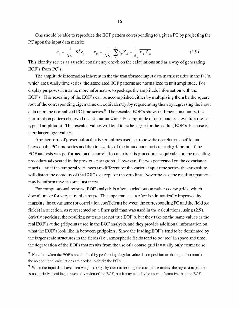
One should be able to reproduce the EOF pattern corresponding to a given PC by projecting the

PC upon the input data matrix:

ek =1

Nl k

XTzk ejk =1

Nl k

xij Ziki =1

N

å =1

l k

x. j Z.k (2.9)

This identity serves as a useful consistency check on the calculations and as a way of generating

EOFÕs from PCÕs.

The amplitude information inherent in the the transformed input data matrix resides in the PCÕs,

which are usually time series: the associated EOF patterns are normalized to unit amplitude. For

display purposes, it may be more informative to package the amplitude information with the

EOFÕs. This rescaling of the EOFÕs can be accomplished either by multiplying them by the square

root of the corresponding eigenvalue or, equivalently, by regenerating them by regressing the input

data upon the normalized PC time series.9 The rescaled EOFÕs show, in dimensional units, the

perturbation pattern observed in association with a PC amplitude of one standard deviation (i.e., a

typical amplitude). The rescaled values will tend to be be larger for the leading EOFÕs, because of

their larger eigenvalues.

Another form of presentation that is sometimes used is to show the correlation coefficient

between the PC time series and the time series of the input data matrix at each gridpoint. If the

EOF analysis was performed on the correlation matrix, this procedure is equivalent to the rescaling

procedure advocated in the previous paragraph. However, if it was performed on the covariance

matrix, and if the temporal variances are different for the various input time series, this procedure

will distort the contours of the EOFÕs, except for the zero line. Nevertheless, the resulting patterns

may be informative in some instances.

For computational reasons, EOF analysis is often carried out on rather coarse grids, which

doesnÕt make for very attractive maps. The appearance can often be dramatically improved by

mapping the covariance (or correlation coefficient) between the corresponding PC and the field (or

fields) in question, as represented on a finer grid than was used in the calculations, using (2.9).

Strictly speaking, the resulting patterns are not true EOFÕs, but they take on the same values as the

real EOFÕs at the gridpoints used in the EOF analysis, and they provide additional information on

what the EOFÕs look like in between gridpoints. Since the leading EOFÕs tend to be dominated by

the larger scale structures in the fields (i.e., atmospheric fields tend to be ÔredÕ in space and time,

the degradation of the EOFs that results from the use of a coarse grid is usually only cosmetic so

8 Note that when the EOFÕs are obtained by performing singular value decomposition on the input data matrix,

the no additional calculations are needed to obtain the PCÕs. 9 When the input data have been weighted (e.g., by area) in forming the covariance matrix, the regression pattern

is not, strictly speaking, a rescaled version of the EOF, but it may actually be more informative than the EOF.

17

that the finer scale structure that would have been revealed by a prohibitively expensive higher

resolution EOF analysis can be filled by the use of this simple procedure. This technique can also

be used to expand the domain of the display beyond what was used in the EOF calculations.

The EOFÕs and PCÕs together define how a given mode contributes to the variability of the

input data matrix. The signs of the two bear a definite relationship to one another, but the sign of

any EOF/PC pair is arbitrary: e.g., if ek and zk for any mode are both multiplied by (Ð1), the

contribution of that mode to the variability in X is unchanged. The sign assigned by the computer

to each EOF/PC pair is arbitrary, but the analyst may have distinct preferences as to how he or she

would like them displayed. For example, if the individual ejkÕs in a given EOF mode all turn out to

be of the same sign (as is not uncommon for the leading EOF), it might be desirable to have that

sign be positive so that positive values of Zik will refer to times or places (i) when xij is positive for

all j. Or the sign convention might be selected to make the EOF (or PC) easy to compare with

patterns displayed in diagrams or tables in previous studies or in the same study. Note that sign

conventions can be specified independently for each EOF/PC pair.

2.6 Statistical significance of EOF’s

The EOFÕs of Ôwhite noiseÕ in which the off diagonal elements in the dispersion matrix are zero

and the diagonal elements are equal but for sampling fluctuations, are degenerate. For Ôred noiseÕ,

in which the correlations between nearby elements in the correlation matrix falls off exponentially,

as in a first order Markov process, the EOFs are families of analytic orthogonal functions. In one

dimension the functions resemble sines and cosines and on a sphere they are the spherical

harmonics (i.e., products of sine or cosine functions in longitude and Legendre polynomials in

latitude). The rate at which the eigenvalues drop off as one proceeds to higher modes depends

upon the ÔrednessÕ of the data in the space domain. Hence EOF patterns with pleasing geometric

symmetries arenÕt necessarily anything to get excited about.

The spatial orthogonality of the EOFÕs imposes constraints upon the shapes of the modes: each

mode must be spatially orthogonal to all the modes that precede it in the hierarchy. The lower the

rank of its eigenvalue the more modes it is required to be to be orthogonal to, and the more likely

that its pattern is dictated by mathematical constraints, rather than physics or dynamics.10 For this

reason many studies emphasize only the leading EOF, and relatively few show results for modes

beyond the third or fourth.

10 The smaller the number of input time series, the fewer the possible ways it has of satisfying these constraints.

As an extreme example, consider the case with just two X time series x1 and x2. If x1 and x2 are positively

correlated in the first EOF they must be negatively correlated in the second EOF and vice versa.

18

The uniqueness and statistical significance of the EOFs is critically dependent upon the degree

of separation between their eigenvalues. For example, if two EOFÕs explain equal amounts of the

total variance, it follows that any linear combination of those EOFs will explain the same amount of

variance, and therefore any orthogonal pair of such linear combinations is equally well qualified to

be an EOF. In the presence of sampling variability a similar ambiguity exists whenever EOFs are

not well separated. The degree of separation required for uniqueness of the EOF modes depends

upon the effective number of the degrees of freedom in the input data, N*, which is equivalent to

the number of independent data points in the input time series. North et al.(1982) showed that the

standard error in the estimates of the eigenvalues is given by

Dl i = l i 2 / N* (2.10)

If the error bars between two adjacent eigenvalues (based on one standard error) donÕt overlap,

there is only a 5% chance that the difference between them could be merely a reflection of sampling

fluctuations.

In practice, (2.10) is difficult to use because the number of degrees of freedom in geophysical

time series is difficult to estimate reliably, even when one takes account of the serial correlation in

the input data by modeling it as a first order Markov process as suggested by Leith (1973).

Therefore, the most reliable way of assessing the statistical significance of EOFÕs is to perform

Monte Carlo tests. One approach is to randomly assign the observation times in the dataset into

subsets of e.g., half the size, and compare the EOFÕs for different subsets against the ones for the

full dataset (or against one another) using an objective measure of similarity such as the spatial

correlation coefficient or the congruence11. By generating 30-100 such subsets it is possible to

estimate the confidence levels with which one can expect that the leading EOFs will retain their

rank in the hierarchy and exhibit prescribed levels of similarity: e.g., the fraction of the monte

carlo runs in which they match their counterparts in a mutually exclusive subset of the data as

evidenced by a spatial correlation coefficient of at least, say, 0.8.

In general, the simpler the structure of a field (i.e., the smaller the number of equivalent spatial

degrees of freedom), the more of the dispersion will be accounted for by the leading EOFÕs and the

larger the degree of separation that can be expected between the leading eigenvalues. Hence,

hemispheric fields of parameters such as monthly mean geopotential height and temperature, which

tend to be dominated by planetary-scale features, are more likely to have statistically significant

leading EOFÕs than fields such as vorticity and vertical velocity, which exhibit more complex

11 The congruence is analogous to the spatial correlation coefficient except that the spatial mean is retained in

calculating the spatial covariance and variances.

19

structures. In this respect, it is worth noting that the number of equivalent spatial dgrees of

freedom is often much less than the number of data points in the grid. For example, the number of

gridpoints in the hemispheric analyses produced at NMC and ECMWF is of order 1000, but the

number of spatial degrees of freedom for, say, 5-day mean maps is estimated to be on the order of

20.

2.7 How large should the domain size be?

The results of EOF analysis are dependent upon the effective number of degrees of freedom in

the domain of the structure. Choosing too small a domain precludes the possibility of obtaining

physically interesting results and choosing too large a domain can, in some instances, preclude the

possibility of obtaining statistically significant results. But before considering this issue in detail,

let us consider the related issue of domain boundaries.

Other things being equal, it is most desirable to use natural boundaries in an EOF analysis or

no boundaries at all (e.g., streamfunction in a global domain, sea surface temperature in an ocean

basin, sea-ice concentration in the Arctic polar cap region). The next best place to put the

boundaries is in regions of low variability (e.g., the 20°N latitude circle for an analysis of Northern

Hemisphere geopotential height variability.

If the domain size is smaller than the dominant scales of spatial organization in the field that is

being analyzed, the structure of the variance or correlation matrix will resemble red noise. The

time series for most gridpoints will be positively correlated with one another, with the possible

exception of those located near the periphery of the domain. In such a situation, one is likely to

obtain, as EOFÕs, the type of geometrically pleasing functions that one obtains form red noise.

The leading EOF will be centered near the middle of the domain and will be predominantly of the

same sign; EOF 2 will have a node running through the middle of the domain, with positive values

on one side and negative values on the other. If the domain is rectangular and elongated in one

direction, the node is likely to run along the shorter dimension. The shapes of the higher modes

are likely to be equally predictable, and equally uninteresting from a physical standpoint.

If the domain size is much larger than the predominant scales of organization, the number of

degrees of freedom in the analysis may decline to the point where sampling fluctuations become a

serious problem. The greater the equivalent number of spatial degrees of freedom of the field that

is being analyzed the greater the chance of obtaining spurious correlations that are just as strong as

the real ones. The fraction of the total variance explained by the leading modes declines, as does

the expected spacing between the eigenvalues, which determines the uniqueness and statistical

significance of the associated EOFÕs. Fortituitous correlations between widely separated

gridpoints are reflected in EOF patterns that fill the domain. The fluctuations at the various centers

of action in such Ôglobal patternsÕ will not necessarily be well correlated with one another.

20

Vestiges of the real structures may still be present in the leading EOFÕs, but they are like flowers in

a garden choked by weeds.

Hence, the optimal domain size depends upon the scale of the dominant structures in the data

field. Horizontal fields such as geopotential height, streamfunction, velocity potential, and

temperature are well suited to EOF analysis in a global or hemispheric domain: fields with smaller

scale structure such as vorticity, vertical motion, cloudiness or precipitation or the eddy field in the

ocean are inherently too complex to analyze in such a large domain. The larger the number of

temporal degrees of freedom, the larger the allowable domain size relative to the dominant spatial

scales of organization.

Another consideration in the choice of domain size (or the number and mix of physical

parameters) in EOF analysis is the shape (or structure in parameter space) of the anticipated

patterns. EOFÕs are orthogonal in the domain of the analysis. Two or more physically meaningful

structures can emerge as EOFÕs only if those structures are orthogonal within the domain of the

analysis: if they are not orthogonal, only the dominant one can emerge.

2.8 Rotated EOF analysis12

For some applications there exists a range of domain sizes larger than optimal for conventional

EOF analysis but still small enough so that the real structure in the data is not completely obscured

by sampling variability. When the domain size is in this range, the EOF patterns can sometimes be

simplified and rendered more robust by rotating (i.e., taking linear combinations of) the leading

EOFÕs and projecting them back on the input data matrix X to obtain the corresponding expansion

coefficient time series.

A number of different criteria have been advocated for obtaining the optimal rotations (linear

combinations) of the EOFÕs. They can be separated into two types: orthogonal and oblique.

Orthogonal rotations preserve the orthogonality of the PCÕs, whereas oblique rotations do not.

Rotation of either type frees the EOFÕs of the constraint of orthogonality, which is often considered

to be an advantage. For a more comprehensive discussion of the methodology for rotating EOFÕs

the reader is referred to Richman (198xx)

A widely used criterion for orthogonal rotation is the Varimax method in which the EOFÕs,

(ek), weighted by the square roots of their respective eigenvalues, are rotated in a manner so as to

maximize the dispersion of the lengths of their individual components:

12 For lack of a universally agreed upon definition of EOFÕs versus PCÕs, rotated EOFÕs are sometimes referred to

as Ôrotated principal components (RPCÕs)Õ in the literature, implying that the time series, rather than the spatial

patterns, have been rotated. In most cases, the rotation has, in fact, been performed on the spatial patterns, in the

manner described in this section.

21

Äejk2 - Äek

2[ ]j =1

M

å2

, where Äejk = l k ejk and

Äek2 =

1M

Äejk2

j =1

M

å , (2.11)

subject to the constraint that the eigenvectors themselves be of fixed length, say Äek2 = 1, which

would require that Äek2 = 1 / M . The optimization criterion has the effect of concentrating as much

as possible of the amplitude of the EOFÕs into as as few as possible of the components of Äek , and

making the other components as close to zero as possible, which is equivalent to making the

rotated EOFÕs (REOFÕs) as local, and as simple as possible in the space domain.13 The REOFÕs

have no eigenvalues as such, but the fraction of the total variance explained by each mode can

easily be calculated. The leading rotated modes account for smaller fractions of the total variance

than their unrotated counterparts, and their contributions often turn out to be so similar that it

makes no sense to rank them in this manner.

If the complete set of EOFÕs were rotated, the individual loading vectors would degenerate into

localized ÔbullseyesÕ scattered around the domain, which would be of little interest. But when the

set is truncated to retain only the R leading EOFÕs the results can be much more interesting. Rough

guidelines have been developed for estimating the optimal value of R based on the size of the

eigenvalues14, but most investigators experiment with a number of values to satisfy themselves

that their results are not unduly sensitive to the choice. If R is too small, the results do, in fact,

tend to be quite sensitive to the choice, but for some fairly wide midrange, they are often quite

insensitive to the choice of R and they are capable of separating the mixture of patterns evident on

the EOF maps to reveal features such as wavetrains and/or dipoles, if they exist. The simplicity of

the REOFÕs, relative to the unrotated EOFÕs often renders them in closer agreement with the

patterns derived from theory and numerical models.

The uniqueness of the rotated EOFÕs does not derive from the separation of their eigenvalues,

but from their role in explaining the variance in different parts of the domain. It often turns out that

they are much more robust with respect to sampling variability than their unrotated counterparts.

The expansion coefficient time series retain their orthogonality, but the REOFÕs themselves are

freed from the constraint of being orthogonal, though in practice, they remain nearly uncorrelated

in space. When the rotation produces the desired results, as many as five or ten of the REOFÕs

may prove to be of interest: more than is typically the case in EOF analysis.

Because of their simpler spatial structure, the REOFÕs more closely resemble one-point

covariance (or correlation) maps than the unrotated EOFÕs from which they are formed. One might

then ask, ÒWhy not simply display a selection of one-point covariance (or correlation) maps in the

13 Matlabª and Fortran routines for Varimax rotation of EOFÕs are available through JISAO.14 For example, when the EOF analysis is based on the correlation matrix, Guttman suggests rotating the PCÕs

with eigenvalues larger than 1.

22

first place?Ó The advantage of the REOFÕs is that they are objectively chosen and, in the case of

orthogonal rotations, their expansion coefficients (PCÕs) are mutually orthogonal.

When the domain size is no larger than the dominant spatial structures inherent in the data,

rotation often has little effect upon the EOFÕs. In some situations, the Varimax solution may be

quite sensitive and difficult to reproduce exactly, but this has not, in our experience, proved to be a

serious problem.

2.9 Choice and treatment of input variables

For handling large input data arrays (e.g., as in dealing with gridded fields of a number of

different variables) it is permissible to condense the input data, for example by projecting the

individual fields onto spherical harmonics or their own EOFÕs and truncating the resulting series of

modes. In this case the analysis is performed on time series of expansion coefficients (or PCÕs).

The resulting EOFÕs can be transformed back to physical space for display purposes. This

sequence of operations is equivalent to filtering the input data in space to retain the largest scales.

Prefiltering the input data in the time domain can serve to emphasize features in certain frequency

ranges: e.g., baroclinic wave signatures in atmospheric data could be emphasized by analyzing 2-

day difference fields, which emphasize fluctuations with periods around 4 days.

Each geophysical field has its own characteristic space/time structure. For example in the

atmosphere, the geopotential and temperature fields are dominated by features with space scales

(wavelengths / 2p) > 1000 km; wind by features with scales between 300 and 1000 km; and

vorticity, vertical motions, and precipitation by features with scales <300 km. Hence, analyses of

temperature and geopotential are well suited for hemispheric or even global domains, whereas an

analysis of a field such as daily precipitation is better suited to a more regional domain. For

analyses that include the tropics, it may be preferable to analyze streamfunction rather than

geopotential because its amplitude is not so strongly latitude dependent.

2.9.1 Special considerations relating to wind15

When wind is used as an input variable for EOF analysis, variance is associated with kinetic

energy. Analysis of the the zonal wind field by itself tends to emphasize zonally elongated features

such as jets, whereas EOF analysis of the meridional wind field tends to emphasize more isotropic

or meridionally elongated features such as baroclinic waves. For some applications it is useful to

consider both components of the wind in the same analysis.

In zonally propagating modes such as Rossby-waves and gravity-waves (with the notable

exception of Kelvin-waves) the zonal and meridional components u and v fluctuate in quadrature

15 The geostrophic wind field can easily be derived from gridded values of the geopotential field.

23

with one another, at a fixed point. For example, consider a train of eastward propagating Rossby-

waves passing to the north of a Northern Hemisphere station. The wave component of the wind

blows from the south as the wave trough approaches from the west. One quarter period later,

when the center of the cyclonic wind perturbations is passing to the north of the station, the local

wind perturbation is from the west, and so on. Hence, south of the Òstorm trackÓ the perturbation

wind field rotates counterclockwise with time, while to the north of the storm track it rotates

clockwise with time. There are two ways of applying EOF analysis in such a situation:

(i) The u and v perturbations can be treated as imaginary complex numbers (i.e., u + iv), in whichcase, separate u and v maps should be presented for the EOF's. The EOF structures associatedwith a given mode appear in the sequence u+ followed by v+ followed by uÐ followed by vÐ, etc.,where u+ refers to the positive polarity of the u pattern, etc. The PC's are complex, the real partreferring to the amplitude and polarity of the u field and the imaginary part to the v field.Propagating waves will be characterized by circular orbits in the PC's with u perturbations leadingor lagging v perturbations by 1/4 cycle. The propagating Rossby-wave described above will berepresented by a single mode.

(ii ) The u and v fields can both be treated as real variables and combined in the input data matrix.The u and v EOF maps can be incorporated into a single vectorial map and the time series will bereal. In this case, two modes, whose PCÕs oscillate in quadrature with one another, will berequired to represent the propagating Rossby-wave described above.

Now consider a standing oscillation of the form

r

V x,y( )coswt , in which r

V involves both

zonal and meridional wind components oscillating in phase with one another, instead of in

quadrature as in the previous example. The second approach described above should be perfectly

adequate for representing such a structure and it is preferable to the complex representation since it

the results are simpler to interpret.

2.10 Exercises:

2.1. Interpret the various matrices in the flow chart for the following applications:

(a) x is a gridded field like 500 mb height and the two domains are space (e.g., the Northern

Hemisphere or the entire globe) and time (e.g., an ensemble of daily data for a group of Januarys).

An individual map can be viewed as a one dimensional column or row of gridpoint values, and a

time series as a specified gridpoint can be also be viewed as a one dimensional row or column of

gridpoint values. M, the shorter dimension may refer either to space or time.

(b) x refers to a set of measurements taken at a particular location at a series of observation times.

24

For example, it might be the concentrations of a group of chemical species. One instantaneous set

of measurements can be represented as a column or row vector, and the time series of the

measurements of a particular chemical species an be viewed as a row or column vector. The

number of chemicals may be greater or less than the number of observation times. The two

domains may be viewed as Ôparameter spaceÕ and time.

(c) x refers to a set of measurements, as in (b) but they are taken at a number of different sites or

stations, all at the same time. From these data we can generate a map for each chemical species. In

this case the two domains are Ôparameter spaceÕ and physical space.

(d) Let the two domains in the analysis (x,y) refer to the two dimensions of a horizontal

distribution of some variable or, for that matter, a picture of the Mona Lisa in a gray scale

converted to numerical values. Let the EOFÕs be functions of x and the PCÕs be functions of y. If

it makes it any easier, imagine the picture to be a time-latitude section or ÒHovm�ller diagramÓ,

whose y axis can be thought of either as time or as Òy–spaceÓ in the picture.

2.2. Suppose you want to perform an EOF analysis of the 500 mb height field in a hemispheric

domain, in which the time dimension is much shorter than the space dimension of the data matrix

X. You want the PCÕs to have zero mean, but not the spatial means of the EOFÕs. How should

you process the data to get the desired results in a computationally efficient way?

2.3. Form a red noise space/time dataset in the following manner. (1) generate M values of about

N random normal time series e1, e2...eN, with a standard deviation of 1.(2) Let the time series

for your first data point x1(t) be the time series e1. For your second data point, use

x2 = ax1 + 1- a2 e2 , for the third

x3 = ax2 + 1- a2 e3, and so on , up to xN. For best results,

let M be at least 300 and N be at least 20. The coefficient a can be varied between 0 and 1. For an

initial value 0.7 will work well. Calculate the temporal covariance matrix, the EOFÕs, and the PCÕs

for two different values of a. What do they look like? How do they depend on a? How would

the results be different for a periodic domain like a latitude circle?

2.4. In an EOF analysis based on the temporal covariance matrix, how would the results

(eigenvalues, EOFÕs and PCÕs) be affected if the order of the data points were scrambled in the

time domain?

25

2.5. Consider the limiting case in which one assigns a weight of zero to one or more of the input

variables to an EOF analysis. How would you interpret the results for those variables?

2.6. The input data matrix consists of temperature data at 100 stations. The temporal standard

deviation, averaged over all stations, is 4 K. The EOF analysis is based upon the temporal

covariance matrix and all stations are weighted equally. The largest eigenvalue has a numerical

value of 400. (a) What fraction of the total variance is explained by the leading mode? (b) What

is the standard deviation of the leading PC time series? (c) Suppose that the analysis is repeated

using the correlation matrix in place of the covariance matrix. What is the largest possible

numerical value of the largest eigenvalue?

2.7. Consider an input data set consisting of climatological monthly mean (Jan., Feb., ....Dec.)

values of tropospheric (surface to 300 mb vertically averged temperature) on a 2° latitude by 2

longitude grid in a global domain. Describe how you would set up an EOF analysis for maximum

computational efficiency? What kind of weighting scheme (if any) would you use? How many

EOF modes would you expect to obtain? Describe the kind of space/time structure you would

expect to observe in the leading EOF/PC pair. What kinds of structures you might expect to

observe in the next few modes? What fraction of the total variance would you expect to be

explained by the leading mode (20%, 50% or 80%)? Explain. Compare these results with what

you might have obtained if you had performed harmonic analysis instead of EOF analysis.

2.8. Year to year variations in the growth of trees is species dependent and it tends to be limited by

different factors in different climates. It tends to be strongly altitude dependent. Tree ring samples

are collected from a variety of species and sites (encompassing a range of altitudes) in Arizona.

Describe how EOF analysis might be used to analyze such samples and speculate on what some of

the EOF modes might look like and what might be learned from them.

2.9. A suite of chemical and aerosol measurements have been made daily at a small to moderate

size inland Pacific Northwest city (the size of Ellensburg) over a period of 20 years. The city has a

pulp mill, some minor traffic congestion, and a serious wintertime pollution problem due to the

widespread use of wood stoves for home heating, which has increased during the period. Thirty

miles up the valley is another city with a nickel smelter that was operating intermittently during the

period. Suppose that the measurements include at least a few chemicals that are specific to each of

these sources, plus some non specific chemicals. Meteorological measurements (wind,

26

temperature, visibility, sky cover, barometric pressure) are available for a number of surrounding

stations, one of which takes daily radiosonde observations. The investigator has access to records

indicating when the pulp mill and the smelter were operating and when they were shut down.

Hospital records are also available indicating daily numbers patients with admitted with respiratory

problems and deaths due to respiratory diseases. Describe how EOF analysis might be used to

analyze these data, and speculate on what some of the EOF modes might look like and what might

be learned from them.

References

Textbooks:

Strang

27

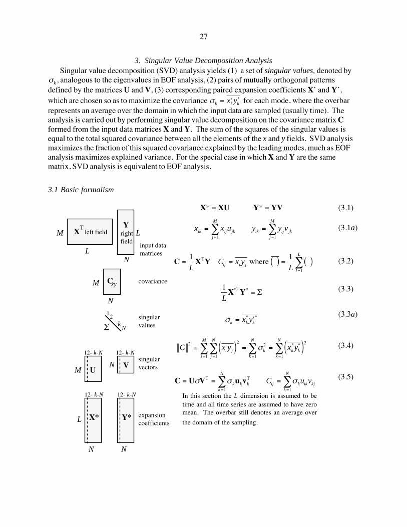
3. Singular Value Decomposition AnalysisSingular value decomposition (SVD) analysis yields (1) a set of singular values, denoted by

sk, analogous to the eigenvalues in EOF analysis, (2) pairs of mutually orthogonal patternsdefined by the matrices U and V, (3) corresponding paired expansion coefficients XÕ and YÕ,which are chosen so as to maximize the covariance

sk = ¢xk ¢yk for each mode, where the overbar

represents an average over the domain in which the input data are sampled (usually time). Theanalysis is carried out by performing singular value decomposition on the covariance matrix Cformed from the input data matrices X and Y. The sum of the squares of the singular values isequal to the total squared covariance between all the elements of the x and y fields. SVD analysismaximizes the fraction of this squared covariance explained by the leading modes, much as EOFanalysis maximizes explained variance. For the special case in which X and Y are the samematrix, SVD analysis is equivalent to EOF analysis.

3.1 Basic formalism

M

12- k-N

M

NS ksingular values

12

M covariance

12- k-N

N Vsingular vectors

LN

N

L

input data matrices

N

Y*

12- k-N

expansion coefficients

X left field Y right field

C

U

N

12- k-N

X*

xy

LT

X* = XU Y* = YV

x x u y y vik ij jkj

M

ik ij jkj

M

= == =

å å1 1

C =1LXTY Cij = xi yj where ( ) =

1L

( )l =1

L

å

1LX*TY* = S

sk = xk

* ¢yk*

C2

º xi yj( )j =1

N

åi =1

M

å2

= sk2

k=1

N

å = xk*yk*( )

k=1

N

å2

C U V u v= = == =

å ås s sT Tk k k

k

N

ij k ikk

N

kjC u v1 1

In this section the L dimension is assumed to betime and all time series are assumed to have zeromean. The overbar still denotes an average over

the domain of the sampling.

(3.1)

(3.1a)

(3.2)

(3.3)

(3.3a)

(3.4)

(3.5)

28

Assuming that the L dimension in section 3.1 refers to time, the input data matrices X and Y

can be defined within different domains and/or on different grids, but they must be defined at the

same times. As in EOF analysis, the left singular vectors comprise a mutually orthogonal basis

set, and similarly for the right singular vectors. However, in contrast to the situation in EOF

analysis, the corresponding expansion coefficients are not mutually orthogonal and the two

domains of the analysis (e.g., space and time) cannot be transposed for computational efficiency.

In contrast to Òcombined EOF analysisÓ (CbEOF) in which two fields X and Y are spliced together

to form the columns of the observation vector, SVD analysis (1) is not directly influenced by the

spatial covariance structure within the individual fields, (2) yields a pair of expansion coefficient

time series for each mode (X* and Y*), instead of a single expansion coefficient time series (Z),

and (3) yields diagnostics concerning the degree of coupling between the two fields, as discussed

in section 3.4.

3.2 The input data and cross-covariance matrices

The cross-covariance matrix that is the input for the singular value decomposition routine is not

necessarily square. Its rows and columns indicate the covariance (or correlation) between the time

series at a given station or gridpoint of one field and the time series at all stations or gridpoints of

the other field. SVD analysis offers the same types of normalizing and scaling options as EOF

analysis (e.g., it can be based on either the covariance matrix or the correlation matrix.)

The total squared covariance, summed over all the elements of C is a measure of the strength of

the relation between the x and y fields. This quantity can be nondimensionalized by forming the

ratio

RMSC º( )

æ

èç

ö

ø÷æ

èç

ö

ø÷

æ

è

çççç

ö

ø

÷÷÷÷

==

= =

åå

å å

x y

x y

i jj

N

i

M

ii

M

ij

N

2

11

2

1

2

1

1

2

(3.6)

which ranges from zero up to a maximum value of the fraction of the variance explained by the

leading EOF, in the event that x and y refer to the same field. For strongly correlated fields this

Ònormalized root-mean squared squared covarianceÓ is typically of order of 0.1 or larger, but even

smaller values may be indicative of a significant relationship between the fields if the number of

independent samples is large.

29

3.3 The singular values

The singular values have units of covariance (i.e., the product of the units of the left and right

fields). The singular value for any mode is equal to the covariance between the expansion

coefficient time series of the left and right fields for that mode, the quantity whose squared value is

maximized in SVD analysis. In addition, the sum of the squares of the singular values is equal to

the square of the Frobenius norm of the covariance matrix, (i.e., the squared covariance, summed

over all the M x N elements of the matrix), and the leading singular value explains the largest

possible fraction of this total squared covariance. That fraction is given by

s12 / sk

2

kå .

For the special case X = Y, the results of SVD analysis are identical to those derived from EOF

analysis and the singular values are identical to the eigenvalues l. However, a larger squared

covariance fraction (SCF) will be accounted for by the first n modes of the SVD analysis than the

variance fraction accounted for by the same first n modes in the corresponding EOF expansion.

For example, suppose that there are five eigenvalues, with values 5, 3, 2, 1 and 1. The first mode

accounts for 5/12 = 43.3% of the variance. The corresponding squares of the singular values are

25, 5, 4, 1 and 1. Hence the same first mode accounts for 25/36 = 70% of the squared covariance.

It will be shown in section 2.5 and 2.6 that high values of SCF for the leading mode obtained from

SVD analysis do not, in themselves guarantee that the relationship between X and Y is statistically

significant. It is also necessary that the normalized squared covariance, as defined in the previous

section, be large.

3.4 Scaling and display of the singular vectors and expansion coefficients

The singular vectors are nondimensional, whereas the expansion coefficient time series have

the same units as the corresponding input data. Like EOFÕs, the singular value vectors U and V

can be scaled and displayed in a number of different ways. Amplitude information can be

incorporated into them, scaling can be undone, signs can be reversed (for uk and vk and the

corresponding expansion coefficient time series simultaneously), just as in EOF analysis. If the

linear transformation of the input data matrices X and Y to obtain the expansion coefficient matrices

XÕ and YÕ is carried out correctly, it should be possible to recover the singular vector patterns for a

given mode by projecting the expansion coefficient tome series upon the input data matrix; i.e.,

uk =1

Lsk

XT ¢yk ujk =1

Lsk

xij ¢yiki =1

L

å =1

sk

x. j ¢y .k (3.7a)

30

vk =1

Lsk

YT ¢xk vjk =1

Lsk

yij ¢xiki =1

L

å =1

sk

y. j ¢x .k (3.7b)

These identities serve as useful consistency checks on the calculations and as a way of recovering

the singular vector patterns from the corresponding expansion coefficient time series. Note that the

patterns for the left field are derived from the expansion coefficient time series for the right field

and vice versa.

The amplitude information inherent in the expansion coefficient time series can be incorporated

into the singular vector patterns for display purposes by mapping the covariance between the

normalized expansion coefficient time series for the left field and the input time series for each

station or gridpoint of the right field and vice versa. These patterns may be viewed as rescaled

versions of the singular vectors that have the same units as the left and right fields. They show

what the patterns in the respective fields characteristically look like when the expansion coefficient

time series of the opposite field has an amplitude of one standard deviation.

In general, two types of covariance (or correlation) maps can be formed from the expansion

coefficient time series derived from SVD analysis: (1) those formed by regressing (or correlating)

the expansion coefficient time series of the left field with the input data for the left field, and the

expansion coefficient time series of the right field with the input data for the right field; (2) and

those formed by regressing (or correlating) the expansion coefficient time series of the left field

with the input data for the right field, and the expansion coefficient time series of the right field

with the input data for the left field. The former are referred to as homogeneous covariance (or

correlation) patterns (i.e., left with left and right with right) and the latter as heterogeneous

patterns. Note that the singular vectors are heterogeneous patterns: they are in some sense the

more fundamental of the two types of patterns because they reveal more directly the relationship

between the left and right fields, which is what SVD analysis is all about. The homogeneous

patterns reveal the structure in a field associated with variations in its own expansion coefficent

time series. Heterogeneous and homogeneous covariance (or correlation) patterns tend to be

similar in shape, but not identical. Homogeneous correlation patterns tend to be stronger than

heterogeneous correlation patterns because they involve relationships within the same field. The

heterogeneous covariance patterns for the various modes are mutually orthogonal in the space

domain, since they are simply rescaled versions of the singular vectors. The same is not true of the

homogeneous covariance maps.

In contrast to the situation in EOF analysis, the expansion coefficient time series are not

mutually orthogonal, though the correlations between them tend to be small. The correlation

coefficient between the left and right expansion coefficient time series provides a useful measure of

the strength of the coupling of the two fields. Often this statistic is displayed together with the

31

squared covariance fraction SCF explained by the mode and the normalized squared covariance

between the two fields.

3.5 SVD analysis of unrelated fields

Consider two unrelated fields as represented by the matrices, X and Y, each having its own

spatial structure as defined by its leading EOFÕs. This situation can be simulated with real data by

randomly scrambling the temporal order of one field relative to the other. The modes obtained

from SVD analysis are entirely spurious in this case, since all the elements of the covariance matrix

would be zero were it not for sampling fluctuations. In the limit, as the sample size becomes

infinitely large the normalized squared covariance and the correlation coefficient between the time

series of the x and y expansion coefficients of the leading mode both tend toward zero, but the

squared covariance fraction SCF explained by the leading mode is indeterminate, since it represents

a fraction of a vanishingly small quantity. Hence, an impressively large value of the SCF for the

leading mode derived from SVD analysis does not, in itself, guarantee that the mode is statistically

significant.

In order to predict what the structure of the leading modes derived from SVD analysis of two

unrelated fields might look like, it is instructive to consider a somewhat roundabout way of

performing the calculations. EOF analysis is first performed on the X and Y input data matrices

separately, and the complete sets of resulting PC time series are used as input data matrices for

SVD analysis (i.e., the elements of the covariance matrix are covariances between PC time series

for the fields of x and y. When the resulting singular vectors are transformed from ÔPC spaceÕ

back to physical space using (2.7), the patterns are identical to those that would have been obtained

if SVD analysis had been performed directly upon the X and Y matrices.

Now consider the PC covariance matrix upon which the SVD analysis is performed. Since the

variances of the PC time series are equal to the corresponding eigenvalues, it follows that the

elements of the covariance matrix with the largest absolute values are likely to be products of x and

y PC time series corresponding to the leading modes in their respective EOF expansions. If one

field is substantially ÔsimplerÕ than the other (i.e., if it has more of its variance concentrated in its

leading EOF, that mode is likely to be associated with the largest squared covariances arising from

the sampling variability. Hence, in the absence of any real relationship between the x and y fields,

the leading modes obtained from SVD analysis resemble the leading EOFÕs of the input data

matrices, particularly those for the simpler field.

32

3.6 Statistical significance

In order to understand the factors that determine the statistical significance of the results derived

from SVD analysis it is covenient to return to the thought experiment in the previous section in

which the time series of the input data matrices are first transformed into a set of orthogonal PCÕs

in the domain of the sampling and SVD analysis is performed upon the covariance matrix generated

from the PCÕs. Let us try to imagine what a typical M x N covariance matrix might actually look

like. The typical magnitudes of the elements of the covariance matrix may be estimated by means

of the product moment formula. The standard deviations of the PCÕs are proportional to the square

roots of the corresponding eigenvalues, which drop off monotonically with mode number.

Whatever relationship might exist between the two fields is usually reflected in the PCÕs of the

leading modes. Hence, the root mean squared amplitude covariances should be expected to drop

off rather steeply with mode number so that the larger values are confined to the upper left corner

of the covariance matrix and the remaining values below, and to the right of them might just as well

be zero, from the point of view of the subsequent singular value decomposition matrix operation.

This is why SVD analysis often yields reproducible results, even when M and/or N are larger than

L. In geophysical applications of SVD analysis, the effective size of the covariance matrix is

usually much smaller than M x N because of the autocorrelation inherent in the x and y fields in the

domains of the patterns. The larger the autocorrelation, the more strongly the variance will be

concentrated in the leading PCÕs. The number of independent samples in the dataset is also

important because it determines the Ônoise levelÕ for the correlation coefficients of the unrelated

PCÕs.16 The lower the background noise level, the more strongly the leading PCÕs, which

presumably contain the ÔsignalÕ will stand out in the covariance matrix above the continuum of

small correlations associated with sampling fluctuations. The smaller the Ôeffective sizeÕ of the

covariance matrix in comparison to the number of independent samples, the more statistically

significant the results.

We are not aware of any formal procedure for evaluating the Ôeffective dimensionÕ of the

covariance matrix, which would be a prerequisite for testing the statistical significance of the

modes derived from SVD analysis. In lieu of a formal statistical test, we have resorted to the

following Monte Carlo procedure. An ensemble of SVD runs on temporally scrambled data is

performed and the ensemble means and standard deviations of the normalized squared covariance,

the squared covariance fraction SCF, and the correlation coefficient between the x and y expansion

coefficient time series are computed. If the leading mode in the SVD analysis is statistically

16 If the number of samples L is less than M (N), it will be possible to determine only L eigenvalues and PC

vectors for the left (right) field, in which case the remaining rows (columns) of the covariance matrix will be

identically equal to zero.

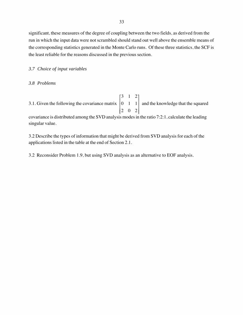
33

significant, these measures of the degree of coupling between the two fields, as derived from the

run in which the input data were not scrambled should stand out well above the ensemble means of

the corresponding statistics generated in the Monte Carlo runs. Of these three statistics, the SCF is

the least reliable for the reasons discussed in the previous section.

3.7 Choice of input variables

3.8 Problems

3.1. Given the following the covariance matrix

3 1 2

0 1 1

2 0 2

é

ë

êêê

ù

û

úúú

and the knowledge that the squared

covariance is distributed among the SVD analysis modes in the ratio 7:2:1, calculate the leadingsingular value.

3.2 Describe the types of information that might be derived from SVD analysis for each of theapplications listed in the table at the end of Section 2.1.

3.2 Reconsider Problem 1.9, but using SVD analysis as an alternative to EOF analysis.

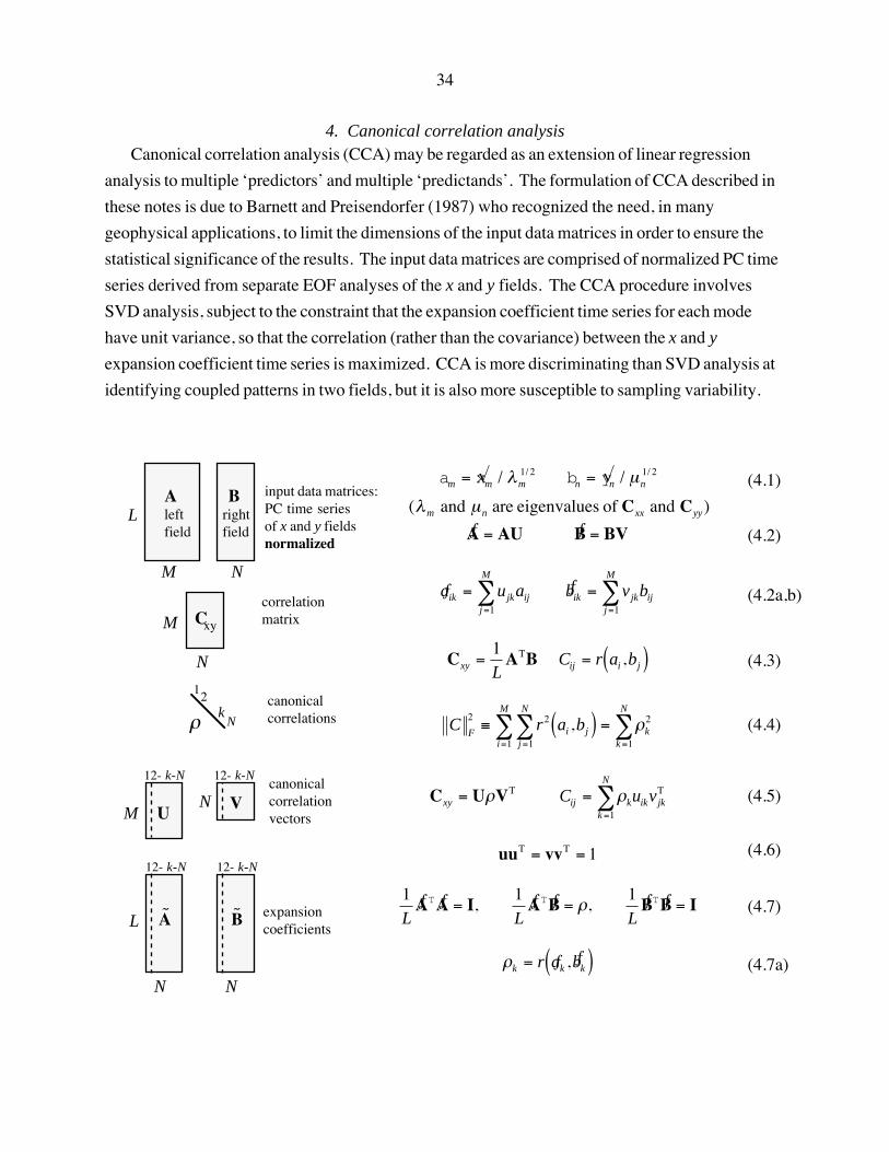
34

4. Canonical correlation analysisCanonical correlation analysis (CCA) may be regarded as an extension of linear regression

analysis to multiple ÔpredictorsÕ and multiple ÔpredictandsÕ. The formulation of CCA described in

these notes is due to Barnett and Preisendorfer (1987) who recognized the need, in many

geophysical applications, to limit the dimensions of the input data matrices in order to ensure the

statistical significance of the results. The input data matrices are comprised of normalized PC time

series derived from separate EOF analyses of the x and y fields. The CCA procedure involves

SVD analysis, subject to the constraint that the expansion coefficient time series for each mode

have unit variance, so that the correlation (rather than the covariance) between the x and y

expansion coefficient time series is maximized. CCA is more discriminating than SVD analysis at

identifying coupled patterns in two fields, but it is also more susceptible to sampling variability.

M

12- k-N

M

Nr kcanonicalcorrelations

12

Mcorrelationmatrix

12- k-N

N Vcanonical correlation vectors

L

N

N

L

input data matrices:PC time series of x and y fieldsnormalized

N

12- k-N

expansion coefficients

A left field

B right field

C

U

N

12- k-N

xy

÷ A

÷ B

am = Ãxm / lm

1/ 2 bn = Ãyn / mn1/ 2

( lm and

mn are eigenvalues of

Cxx and

Cyy)

ÄA = AU ÄB = BV

Äaik = ujkaijj =1

M

å Äbik = vjkbijj =1

M

å

Cxy =1LATB Cij = r ai ,bj( )

CF

2º r 2 ai ,bj( )

j =1

N

åi =1

M

å = rk2

k=1

N

å

Cxy = UrVT

Cij = rkuikk=1

N

å vjkT

uuT = vvT = 1

1LÄAT ÄA = I,

1LÄAT ÄB = r,

1LÄBT ÄB = I

rk = r Äak , Äbk( )

(4.1)

(4.2)

(4.2a,b)

(4.3)

(4.4)

(4.5)

(4.6)

(4.7)

(4.7a)

35

4.2 Input data matrices

Prior to performing CCA the left (x) and right (y) fields are expanded in terms of EOFÕs,

which may be based on either the covariance matrix or the correlation matrix.17 The resulting

principal component matrices are subjected to two procedures:

¥ normalization to make the variance of each mode equal to unity. Hence all input time seriesare weighted equally in CCA regardless of how much of the variance of their respectivepatterns they account for.

¥ truncation to reduce the number of CCA modes among which the degrees of freedom in the xand y fields must be shared. The number of independent samples in the time domain much bemuch larger than the smaller of M or N in order to ensure the reproducibility of the results. Inchoosing the number of modes to be retained as input to CCA, one is faced with a tradeoffbetween statistical significance, which argues for as few modes as possible, and the fraction ofthe variance of the original input matrices X and Y to be retained in the analysis, which arguesfor as many as possible. The number of modes will be determined by the dimension of thesmaller field (in Ònormalized PC spaceÓ).

After these operations, the input matrices no longer contain the information necessary to enable

one to recover the X and Y matrices from which they were derived. To indicate that they are no

longer equivalent, in any sense to the original input data, they are denoted here by different letters

A and B. After normalization they are dimensionless, as are all the other matrices in the diagram in

section 4.1. The remainder of the CCA formalism based on the Barnett and Preisendorfer (BP)

method is disarmingly similar to SVD analysis, as described in the previous section.

4.3 The correlation matrix

Because of the normalization of the ak and

bk , the elements of the covariance matrix are

correlation coefficients between the PCÕs of the left and right fields. Since the input variables are

mutually orthogonal within each of the fields, the Frobenius norm of the correlation matrix may be

interpreted as the fraction of the total variance of A that is explained by B and vice versa. This total

squared correlation is, perhaps, a more natural measure of the strength of the relationship between

17 CCA can be performed upon the X and Y matrices directly, without transformation to PCÕs or normalization.

In this more general case, the matrix used as input to the SVD operation is of the form

ÃCxy º Cxx-1/2CxyCyy

-1/2 and the

interpretation of the canonical correlation vectors is more involved than the one presented here in section 3.4. In

general Cxx and

Cyy are both of full rank and invertible only if L exceeds the larger of M and N. In the Barnett and

Preisendorfer formulation described here, Cxx and

Cyy reduce to identity matrices and the requirement that L>M, N is

satisfied, since the number of PCÕs recovered from the preliminary EOF analysis cannot be larger than L.

36

the left and right fields than the normalized squared covariance defined in section 2.2.18

4.4 The canonical correlations

Because of the constraint imposed in CCA that the expansion coefficient time series have unit

amplitude, the singular values may be interpreted as correlation coefficients and are referred to as

canonical correlations. The singular value decomposition operation encapsulated within CCA

reapportions squared correlation (or explained variance) in C

F

2 so that as much as possible of it is

carried by the leading mode, as much as possible of the remainder by the second mode, etc. The

sum of the squares of the canonical correlations are equal to the total squared correlation in all the

elements of C.

4.4 The canonical correlation vectors and the corresponding expansion coefficients

The orthogonality of the canonical correlation vectors follows from the fact that they are the

singular vectors of the correlation matrix. Hence, (4.2) involves an orthogonal rotation of the PC

time series to obtain the CCA expansion coefficient time series. Since both sets of time series have

unit variance, it follows that the canonical correlation vectors must themselves be of unit length.

The mutual orthogonality expansion coefficient time series in normalized PC space can be

rationalized in the following manner.19 The expansion coefficient time series Äa1 is the linear

combination of the am that explains the maximum possible amount of squared correlation between

A and B and the largest possible fraction of the combined variance of the bn time series. If Äa2 is to

explain as much as possible of the residual variance, it must be orthogonal to Äa1. The argument

can be extended to subsequent modes and to the Äbk.

Applying (3.x) to the canonical correlation vectors, it is apparent that

ujk =1rk

r a·j , Äb·k( ), vjk =1r

r b·j , Äa·k( )Hence, in the terminology developed in section 2.x, the canonical correlation vectors may be

viewed as heterogeneous correlation patterns, scaled by the inverse of the corresponding canonical

correlation. Analogous expressions can be derived relating the canonical correlation vectors to the

homogeneous correlation patterns. Multiplying (3.2a,b) by aij and bij , respectively, averaging

over time, and exploiting the orthonormality of the PC time series yields

18 The statistical significance of the Frobenius norm can be assessed by comparing it with its counterparts derived

from an ensemble of Monte Carlo runs in which the order of the time series in one of the input matrices is

scrambled.19 As an alternative proof it can be shown that, in general, the product of two orthogonal matrices is an

orthogonal matrix. Hence, if A and U are orthogonal, it follows that ÄA is orthogonal, and similarly for B, V and ÄB

37

ujk = r a·j , Äa·k( ), vjk = r b·j , Äb·k( )

Hence, the canonical correlation vectors are the homogeneous correlation patterns in normalized

PC space and the homogeneous correlation patterns in that space are essentially the same patterns,

rescaled by multiplying them by their respective canonical correlations. (The heterogeneous

patterns will generally be weaker than their homogeneous conterparts because the canonical

correlations will generally be smaller than one.

Homogenous and heterogeneous covariance maps in physical space (as opposed to normalized

PC space) can be obtained by regressing the CCA expansion coefficients directly upon the x and y

fields (i.e., without explicit reference to the PCÕs20). The corresponding correlation maps can be

generated in two different ways, which are likely to yield slightly different results: (1) by

correlating the CCA expansion coefficients with original x and y fields or (2) by correlating them

with x and y fields reconstructed from the truncated set of PCÕs weighted by the square roots of

their respective eigenvalues. Since the reconstructed fields have less variance than the total fields,

the correlations obtained by the second method will be stronger. The homogeneous correlation

maps obtained by the second method constitute the appropriate spatial representation of the

canonical correlation vectors. The homogeneous and heterogeneous correlation maps are not

mutually orthogonal in physical space but the heterogeneous correlation maps generated by the

second method should be equivalent to the corresponding homogeneous correlation maps times the

corresponding canonical correlation.

4.5 How many PC’s should be used?

The optimal number of PC time series of the x and y fields to use as input for CCA can be

determined by experimentation or by ad hoc Ôrules of thumbÕ, such as retaining a sufficient number

of PCÕs to retain 70% of the variance of the original fields. If too few PCÕs are retained, the

canonical correlation patterns will be too constrained and they probably will not be able to account

for a sufficient fraction of the variance of the x and y fields to be of physical significance. On the

other hand, if too many modes are included, the statistical significance of the analysis is likely to be

compromised. Of particular importance with regard to statistical significance is the dimension of

the smaller of the input matrices (say, N), for it is that dimension that determines the number of

CCA modes among which the degrees of freedom inherent in the input data will be shared. In

order to ensure the statistical significance of the results, N must be much smaller than the number

of independent samples L* .

The canonical correlation of the leading mode increases monotonically with the number of PCÕs

retained in the smaller of the input data matrices (say, N) and approaches 1 as N/L* approaches 1.

20 The fact that the PC matrix was truncated doesnÕt affect the results because the CCA expansion coefficients are

uncorrelated with the PC time series that are not included in A and B.

38

The squared covariance fraction (SCF)21 usually increases as the first few beyond the leading one

PCÕs are incorporated into the analysis, allowing the canonical correlation vectors more flexibility

in representing the dominant coupled modes of variability in the data. Once the dominant patterns

are well represented, the incorporation of additional modes should have little effect upon the shape

of the leading mode or upon its SCF. When N increases to the point where it is no longer small in

comparison to L* , SCF the leading CCA mode becomes increasingly influenced by sampling

variability. The deterioration of the statistical significance is reflected in an increasing complexity

of the canonical correlation vectors (e.g., more Ôcenters of actionÕ) and a decline in the SCF; both

consequences of the increasing role of the less prominent EOFÕs, which account for only small

fractions of the variances of their respective fields. If L is sufficiently large and the coupling

between the x and y fields is sufficiently strong, there is likely to be a fairly broad range of

truncations N for which CCA yields similar patterns, similar values of SCF and even quite similar

canonical correlations. But if these conditions are not met, the CCA solutions may prove to be

quite sensitive to the choice of N throughout its full range, in which case CCA may not be the

method of choice.

4.6 Statistical significance of CCA modes

The thought experiment conducted at the beginning of section 3.6 can be readily adapted to

CCA. The only difference is that in this case, the PCÕs used to form the covariance matrix are

normalized so that the covariance matrix is, in effect, the correlation matrix between the PCÕs. In

this case, it is evident that the r.m.s. amplitude of the elements of the matrix do not fall off as

rapidly with row or column number as they do in the case of SVD analysis, so that the Ôeffective

dimensionÕ of the matrix will be larger than in the case of SVD. (Unless the number of

independent samples is fairly large, the effective dimension of the matrix may not be much smaller

than M x N). In the Barnett and Preisendorfer method, the rows and columns associated with the

less important PCÕs are zeroed out so that the size of the matrix is forcibly reduced. In the event

that the elements rows and columns that are zeroed out are not small to begin with, the results will

be truncation dependent.

Let us consider two fields as represented by the matrices, X and Y, each having its own spatial

structure as defined by its leading EOFÕs but with one of the matrices scrambled in the time domain

so that there is no statistically significant relationship between the two fields. The PC matrices are

truncated at M and N modes, respectively, and SVD analysis is performed, with and without

normalizing the PC time series. The modes obtained from the former may be interpreted as CCA

21 The SCF for a CCA mode is the sum of the squares of its heterogeneous correlation coefficients divided by the

number of gridpoints or stations.

39

modes and those from the latter as SVD analysis modes, whose properties were discussed in

section 3.5. Whereas the dominant PCÕs are likely dominate the structure of the leading SVD

analysis modes, all PCÕs participate equally in determining the structure of the CCA modes. The

canonical correlations will be higher than the corresponding correlation coefficients derived from

SVD analysis because the normalized PCÕs can all be used effectively to ÔfitÕ the spurious structure

in the covariance matrix, whereas the smaller of the unnormalized PCÕs have much less influence

than the larger ones.

The Monte Carlo test described in section 3.6 can equally well be applied to CCA...

4.7 Relative merits of CCA and SVD analysis

END

40

1.12 Detection of standing oscillations vs. normal mode solutions

1.13 Detection of normal modes

EOF analysis can be extended in several different ways to ehhance its effectiveness in

representing normal mode type space/time patterns. These methods make it possible to represent

such a pattern in terms of a single mode as opposed to a pair of modes.

(a) Extended EOF analysis

The observations at n sequential times are spliced together to form an extended input data

vector. Hence the observations for the nth observation time appear in all the extended input data

vectors from the first up to and including the nth. Each of the resulting EOFÕs consists of n

patterns, which follow one another in chronological order. If the time span n dt, where dt is the

time interval between observations is short in comparison to the time scale of the fluctuations, the

patterns will all look alike and nothing will have been gained by doing extended EOF analysis. But

if it is comparable to it, one might hope to see an orderly evolution of the patterns in the sequence

which would reveal the normal mode structure. Multi-channel singular spectrum analysis may be

viewed as an elaboration of this approach.

(b) EOF analysis in the frequency domain

The covariance matrix in section 1.1 is replaced by the cross spectrum matrix Fxy(f). Diagonal

elements are power spectra and Fyx = Fxy for all the off-diagonal elements, so the matrix is

Hermitian. The frequency band is chosen to be fairly wide so as to encompass a substantial

fraction of the variance of x. Diagonalization of the cross-spectrum matrix yields real, positive

eigenvalues, which can be interpreted in terms of the contributions of their respective EOFÕs to the

power (variance) in that frequency band. The EOFÕs will, in general, be complex. In a normal

mode type solution the real and imaginary parts would appear in quadrature with one another in the

time domain. Separate analysis can be performed for different frequency bands. This method

does not yield PC's directly, although in some cases it may be possible to generate time series that

resemble PC's.

(c) EOF analysis of complex time series

To the existing real time series x, imaginary components are added which represent the time

derivative at each observation time. The time derivative can be estimated in either of two ways:

(i) as a centered difference between the values of x at the two adjacent observation times, or (ii) in

terms of the Hilbert transform. In (i) the time step dt should be chosen such that the time

41

derivative will emphasize the frequency range of particular interest in the study. For best results, it

should be roughly 1/4 as long as the period of interest. (If decimation is performed to reduce the

sampling frequency, a lowpass filter should be applied beforehand.) The Hilbert transform (ii)

weights all frequencies equally in computing the time derivative.

In forming the dispersion matrix, the real and imaginary parts of the time series are assigned

equal weight. As in (b) it is Hermitian, so the eigenvalues are real and positive and the EOF's are

complex. In this case, complex PC time series can be generated from the formulas in section 1.1.

An arbitrary phase angle can be added to each of the EOF/PC modes. One way to render them

unique is to choose that angle so that the real part of the EOF is as large as possible, thus ensuring

that any standing oscillations that might be present will appear in the maps for the real component.

In an idealized normal mode patterns, the PC would trace out a counterclockwise circular orbit

centered on the origin in the complex plane, with the real part of the EOF appearing in its positive

polarity when the PC crosses the x axis, the imaginary part appearing in its positive polarity 1/4

cycle later, when the PC crosses the y axis, and so on.

As an alternative to dealing with complex arithmetic, the time derivatives at each station or

gridpoint can simply be appended to the observations themselves to create an extended input data

matrix with twice as many columns as there are stations or gridpoints. Each EOF then consists of

two patterns: one for x and the other for its time derivative. In this case the PC's are real and

describe the amplitude and polarity of the x part of the EOF. The time derivative part varies in

quadrature with the PC's.