1

Optimal Training for Residual Self-Interference for

Full-Duplex One-way Relays

Xiaofeng Li, Cihan Tepedelenlioglu Member, IEEE,

and Habib Senol Member, IEEE

Index Terms

Full-duplex relays, residual self-interference, maximum likelihood estimation, optimal training sequence,

Toeplitz matrix, frequency-selective channels, multiple relays

Abstract

Channel estimation and optimal training sequence design for full-duplex one-way relays are investigated.

We propose a training scheme to estimate the residual self-interference (RSI) channel and the channels be-

tween nodes simultaneously. A maximum likelihood estimator is implemented with Broyden-Fletcher-Goldfarb-

Shanno (BFGS) algorithm. In the presence of RSI, the overall source-to-destination channel becomes an inter-

symbol-interference (ISI) channel. With the help of estimates of the RSI channel, the destination is able to

cancel the ISI through equalization. We derive and analyze the Cramer-Rao bound (CRB) in closed-form by

using the asymptotic properties of Toeplitz matrices. The optimal training sequence is obtained by minimizing

the CRB. Extensions for the fundamental one-way relay model to the frequency-selective fading channels and

the multiple relays case are also considered. For the former, we propose a training scheme to estimate the

overall channel, and for the latter the CRB and the optimal number of relays are derived when the distance

between the source and the destination is fixed. Simulations using LTE parameters corroborate our theoretical

results.

I. INTRODUCTION

Due to the growing demands on wireless bandwidth, the need for high spectral efficiency has

become more urgent. In-band full-duplex (FD) relays, which transmit and receive simultaneously in

Xiaofeng Li and Cihan Tepedelenlioglu are with the Department of Electrical, Computer and Energy Engineering, Arizona StateUniversity, Tempe, AZ, 85287, USA (email: xiaofen2,cihan@asu.edu).

Habib Senol is with Department of Computer Engineering, Faculty of Engineering and Natural Sciences, Kadir Has University,Istanbul 34083, Turkey (e-mail: hsenol@khas.edu.tr).

arX

iv:1

709.

0614

0v2

[ee

ss.S

P] 1

8 Ju

l 201

8

2

the same frequency band, offer a viable solution since they theoretically have the ability to double the

spectral efficiency, compared to half duplex relays. In practice, however, the relay receives strong self-

interference in FD mode, which is challenging to overcome. Recently, self-interference cancellation

techniques have been developed with great promise [1]–[3]. With these techniques, the self-interference

can be canceled by estimating the self-interference channels [4]–[6] in FD mode, or be suppressed with

null-space methods in MIMO systems [7]. However, despite these advances, residual self-interference

(RSI) still exists after the self-interference cancellation [3], [7]–[9]. Therefore, accurate channel esti-

mation in the presence of RSI is required at the destination to further improve the system performance

by canceling RSI.

Several works analyze the system performance in the presence of RSI with different criteria such as

interference power, outage probability, and bit error rate (BER) [9]–[12]. Reference [10] investigates

the outage probability of an amplify-and-forward (AF) FD relay. Reference [9] takes advantages of

multiple antennas to suppress the RSI power using a null-space pre-coding matrix. References [11]

and [12] analyze the diversity and the capacity of FD relays in the presence of RSI. However, these

works do not consider the cancellation of the RSI. Some of the works assume perfect channel state

information (CSI) [10], [11] while others assume imperfect CSI [9], but they do not mention training

schemes for FD systems. As shown by the results of these works, the system performance suffers

from the RSI since it is still quite high as compared to the desired received signal, and does not yield

good performance when treated as noise. In [10], the authors assume that the RSI power is as high as

10 dB than the desired signal power and also results in inter-symbol interference (ISI) in AF relays.

References [3], [8], and [9] report that the power of RSI may be as high as 30 dB than the noise floor

even after applying self-interference cancellation. As the estimation error in analog cancellation [3],

RSI cannot be further estimated at the relay, which motivates incorporating the RSI into the end-to-end

channel model, and then estimating it, and removing it at the destination.

In addition to the one-way relay system, in-band FD can also be applied in two-way relays in which

two sources exchange their messages through the relay [13]–[17]. The achievable rates of FD relays

and half duplex relays are compared in [13]. References [14], [15] consider the channel estimation

error as an additive noise terms and analyze the effect of it without showing specific training schemes.

In contrast to them, we propose training schemes for the FD relay system in this paper. Reference

3

[16] considers an amplify-and-forward FD two-way relay system in the presence of RSI with multiple

antennas. However, [16] assumes the RSI can be eliminated by designing precoding matrices where

the product of the precoding matrix and the RSI channel matrix equals to zero, which is impractical.

The channel estimation problem for RSI in FD two-way relays is addressed in [17]. The RSI channel,

which is the loop self-interference channel from the relay receive antenna to its transmit antenna after

self-interference cancellation, and the channels between nodes are estimated simultaneously at the

sources, and the asymptotic behavior of the Fisher information is analyzed.

The AF FD relay system can be also combined with MIMO [18], [19]. In the MIMO case, the signal

distortion caused by hardware impediments like the limited dynamic-range of non-ideal amplifiers,

oscillators, ADCs, and DACs has to be considered [20]–[24] when modeling the RSI channel. However,

with sufficient passive self-interference suppression and analog cancellation in RF [3], the distortion can

be ignored [8], which leads to a Gaussian model for the RSI channel [16], [25], [26]. The Gaussian

model still works when the distortion has to be considered. That is because the distortion is well

modeled as additive Gaussian noise terms which can be incorporated into the system noise variance

[20].

From the RSI channel estimation point of view, reference [26] proposes two methods for the RSI

channel in an AF relay system where the destination is equipped with massive MIMO. In the first

method the authors consider the case where the RSI channel is estimated by the relay itself, and in the

second method the base station estimates the RSI channel. However, in their system model, the RSI

is incorporated into the noise term and the ISI caused by the RSI is treated as noise. A conference

version of this manuscript [27] proposes a maximum likelihood (ML) estimator for the RSI channel and

derives the Cramer-Rao bounds (CRBs). In this work, we further analyze the CRB by using asymptotic

properties of Toeplitz matrices and design the optimal training sequences. We also extend our training

method to the case in which the channels in the relay system are frequency-selective and the case

of multi-relay systems, which were not considered in [27]. Reference [17] investigates the channel

estimation problem in FD two-way relays which is fundamentally different than the one-way relay

setting considered herein. We consider the one-way relay case where only the source sends training

and the relay forwards in contrast to [17] which considers a specific training scheme in two-way

relays in where the relay sends its own training sequence. In this paper we eliminate one parameter of

4

interest and integrate out a nuisance parameter, making the objective function depend on only a single

parameter. In contrast, the ML estimator in [17] is with respect to multiple parameters due to the

differences in the system model. From the analysis point of view, we are able to obtain a closed-form

expression for the CRB and find the optimal training sequence accordingly, which is a step further

than the Fisher information analysis in [17]. Moreover, we have extensions to the frequency-selective

and multi-relay cases. The closed-form expression for the CRB is also extended in the multi-relay

case to determinate the optimum number of relays.

In this work, we consider an AF FD one-way relay system with the relay working in FD mode. The

RSI in the relay propagates to the destination, creating an end-to-end ISI channel. We further cancel the

RSI at the destination by estimating the RSI channel and applying equalization. Different from studies

which focus on canceling the self-interference at the relay itself, we reduce the complexity burden at the

relay and aim to cancel the interference at the destination. Thus, the destination performs the estimation

and cancellation operations. To estimate the RSI channel as well as the channels between nodes, an ML

estimator is proposed, which is formulated by maximizing the log-likelihood function through a quasi-

Newton method. The CRBs are derived in closed-form. By using asymptotic properties for Toeplitz

matrices, we are able to find the corresponding optimal training sequences through minimizing the

CRB. We also extend our training method and analysis for the basic relay system to the case when the

channels between nodes are frequency-selective and the case of multiple relays. The main contribution

of this paper is that the effective end-to-end channel of the FD relay system in the presence of RSI

is investigated and an ML estimation of the effective channel including the RSI channel is proposed.

The CRB and optimal training sequences are also analyzed in closed-form. We will briefly explain

how to address practical issues such as the synchronization of the relay received signal and the RSI

signal, and the possibility of clipping of the received signal due to the relay gain in Section II.

The rest of the paper is organized as follows: Section II describes the system model of an AF FD

one-way relay system. Section III proposes the training scheme and the ML estimator. The CRBs are

derived and analyzed in Section IV, and the optimal and the approximately optimal training sequences

are also discussed. Section V and VI extend our training method to frequency-selective channel and

multi-relay case. Section VII shows the numerical results and Section VIII concludes the paper.

5

II. SYSTEM MODEL

We consider a system consisting of a source, a relay, and a destination, without any direct link

between the source and the destination, as shown in Figure 1. Amplify-and-forward relay protocol is

adopted. The relay uses two antennas, one receiving the current symbol while the other one amplifying

and forwarding the previously received symbol, to operate in FD mode [10]. The channel coefficients

between the source and the relay, and the relay and the destination are hsr and hrd respectively. The

two channels between nodes are assumed to be flat fading modeled by independent complex Gaussian

random variable with zero means and variances σ2sr, σ

2rd, respectively. A separate pre-stage is assumed

to gather the information of the self-interference channel to perform analog and digital cancellation

methods in the next transmission stage [3], [26]. During the transmission, the self-interference is

reduced in RF with analog cancellation methods until the residual self-interference power falls in

the ADC dynamic range, and then is further suppressed by digital methods. However, despite these

suppression methods, the RSI is still present at the destination. We consider the RSI as the residual

(error) through either analog cancellation only or analog-plus-digital cancellation. The non-zero residual

is an unavoidable result of the self-interference cancellation. Even though the LoS component is largely

canceled, the RSI power is still not small enough to be treated as noise, and is often higher than the

desired signal power [3], [8]. Moreover, the RSI makes the overall end-to-end channel an ISI channel

at the AF relay, even when the channels on all links are flat fading. Thus, estimating the RSI at the

destination is needed for equalizers to alleviate the ISI at the destination receiver.

Since the line of sight (LoS) component of the self-interference varies very slowly, it can be much

reduced by the RF cancellation, which means the reflected multi-path component dominates the RSI

in the transmission stage [25], [26]. Under the assumption that the LoS component is reduced and

the bulk of the interference is from scattering components, the RSI channel hrr can be modeled as a

complex Gaussian random variable with zero mean and variance σ2rr [25]. Moreover, the RSI channel is

also assumed to be frequency-flat and time-invariant within blocks. The Gaussian model is also used by

[16] and [26] for mathematical tractability. In our system model, we assume that hrr is time-invariant

and flat fading in one transmission block and varies from block to block. The Gaussian assumption

is used in the simulations to generate realizations of the channels for multiple blocks but not in the

derivation of our training scheme and analysis. Different channel models such as Rician model for the

6

Fig. 1. A full-duplex one-way relay system.

self-interference channel before active cancellation [8] can also be adopted.

We assume the processing delay for the relay to forward its received symbols is τ0 which is a

integer multiple of the symbol duration Ts, i.e τ0 = mTs, m = 1, 2, · · · . The processing delay τ0 is a

deterministic system parameter and can be known at the system design level once the hardware and the

self-interference cancellation approaches are chosen. We introduce an artificial additional processing

delay to make τ0 an integer multiple of the symbol duration, which can be implemented by analog

delay filters [28]. With the synchronized signal, the resulting discrete-time equivalent channel model is

sparse with zero coefficients and can simplify the analysis. We use τ0 = mTs in the derivation of the

ML estimator and CRB analysis but we show that it is possible to update our ML estimator and CRB

derivation and analysis with an additional unknown parameter τ0 (which means no synchronization at

the relay) in Appendix II. Let the transmitted signal at the relay be tr[n] = αyr[n−m] where α is a

real and positive power scaling factor. The factor controls the stability of the system through scaling

the relay transmit power. We will discuss the choices of it later in this section. At the destination, the

received symbol at the nth time interval is

yd[n] = hrdt[n] + nd[n] = hrd(αyr[n−m]) + nd[n]

=∞∑k=1

hθk−1x[n− km] +∞∑k=1

dθk−1nr[n− km] + nd[n] n = 0, 1, · · · (1)

where yr[n] = hsrx[n] + αhrryr[n − m] + nr[n] is the nth received symbol at the relay. x[n] is the

transmitted signal of the source and satisfies E[|x[n]|2] = Ps where Ps is the transmit power of the

source and incorporates the path loss. For brevity, we define d := αhrd, h := αhsrhrd and θ := αhrr.

Noise terms nr[n] and nd[n] are complex Gaussian with zero mean and variance σ2r and σ2

d respectively.

If there is no RSI, the effective end-to-end channel h is the overall channel for the system. However,

7

the self-interference link θ forms a feedback at the relay, which makes the overall channel a single

pole infinite impulse response (IIR) channel and causes ISI. Additionally, the effective noise at the

destination is colored with correlations that depend on the pole. The overall IIR channel has channel

taps [h, 0, · · · , 0︸ ︷︷ ︸m terms

, hθ, 0, · · · , 0︸ ︷︷ ︸m terms

, hθ2, 0, · · · ]T . We can see that m only affects the position of the non-zero

coefficients, which means that m has no effect on calculating the gradients in Section III-B. Moreover,

in Section IV-B, the zero coefficients have no contribution to (25) which is the key component in the

CRB analysis. Thus, assuming m = 1 is without loss of generality.

The self-interference cancellation at the relay should be such that |θ| < 1 is possible with proper

choice of α. Such α keeps the system stable and guarantees finite average relay transmit power. The

average relay transmit power is calculated as

E[tr[n]t∗r [n]] = α2

∞∑k=1

(α2|hrr|2)(k−1)(Ps|h|2 + σ2

r

)= α2 Ps|h|2 + σ2

r

1− α2|hrr|2. (2)

Define Pr as the maximum relay transmit power. The condition for the stability of the system is given

by [29]

E[tr[n]t∗r [n]] ≤ Pr, (3)

where the expectation in (3) is with respect to the noise. By solving (3), α should satisfy α2|hrr|2 =

|θ|2 < 1. However, in a channel estimation scenario, the expectation value of hrr is used instead of its

instantaneous value in α. We can choose α to satisfy a long term condition E[α2|hrr|2] < 1 which leads

to α2σ2rr < 1. The RSI variance σ2

rr can be obtained at the pre-stage. Using the variance of the RSI

channel instead of its realizations is a common problem in AF FD relays since the RSI is considered

as the residual error which cannot be further estimated after all the self-interference cancellation

approaches. Note that RSI channel realization might exceed some threshold. If that happens, α can be

adjusted to make the relay transmit with its maximum power. This will lead to clipping and distortions

but not instability. In addition, the clipping case happens with small probability since the RSI channel

has small variance [3] which limits the dynamic range of the realizations. To further reduce the clipping

probability, a fixed power margin between the relay gain power and the maximum power can be made

on α to increase the threshold. Therefore, we do not incorporate these distortions in our system model

8

and analysis. We can choose α to first normalize the received signal power, and then to amplify the

signal power to Pr which is the maximum power the relay can use given the power margin. Such an

α is given by

α2 =Pr

Ps + Prσ2rr + σ2

r

. (4)

Since the non-zero coefficients θk−1 at the kth taps of the IIR channel decrease in amplitude with

increasing tap index k, we can assume that most of the energy (e.g. 99%) is contained in a finite length

of the overall channel impulse response [10]. Define L as the effective length of the overall impulse

response which is h[k] := hθk, k = 0, · · · , L − 1. Thus, we use a block-based transmission with a

guard time of L symbol intervals to avoid inter-block interference [17]. At the receiver, it receives

N + L symbols and discards the last L symbols. Without loss of generality, the block length N is

assumed to be far greater than L, so the rate loss due to the guard time is negligible. With the effective

length L and block-based transmission, we can truncate the IIR channel.

Let Hθ be the matrix form of the channel in one block, which is given by an N × N Toeplitz

matrix with first column [1, θ, θ2, · · · , θL−1, 0, · · · , 0]T and first row [1, 0, · · · , 0].

We rewrite the output in terms of x := [x[0], · · · , x[N − 1]]T and y := [yd[1], · · · , yd[N ]]T as:

y = hHθx+ dHθnr + nd, (5)

where nr and nd are noise vectors composed of independent samples from the same distribution as

nr[n] and nd[n] respectively. As can be seen from the matrix expression, hHθ is the overall channel

and the sum of the last two terms in (5) is the colored noise. Thus, the overall channel becomes an ISI

channel. In (5), we assume distortion of the signal caused by hardware impediment is negligible due

to sufficient passive self-interference suppression and analog cancellation in RF [8]. However, if the

distortion has to be considered, (5) does not change because the distortion can be incorporated as part

of the noise. To be specific, the distortion from the transmitter and the receiver are incorporated into

the colored noise term dHθnr and additive noise term nd respectively [20]. Since we have explicitly

labeled the noise variances of nr and nd as σ2r and σ2

d respectively, the incorporation of the distortion

can be captured by modifying the noise variance values.

9

III. CHANNEL ESTIMATION

A. Maximum Likelihood Formulation

We now derive the ML estimator of h and θ for a given training sequence x. We are only interested in

h and θ since knowing them is enough for detection and equalization. In (5) we have three parameters

h, θ and d. The coefficients of the desired signal x is hHθ which only contain h and θ while d appears

in the colored noise term dHθnr. When detecting x, d is not necessary. For example, at high SNR,

a zero-forcing detector can be used which is obtained by using h and θ to calculate the inverse of

hHθ. We set d as a nuisance parameter and integrate out the nuisance parameter from the likelihood

function which is an established method [30] to deal with it in the likelihood function. We have

p(y|h, θ) =

∫p(y|h, θ, d)p(d)dd. (6)

Since p(y|h, θ, d) and p(d) are Gaussian distributed, it is shown in Appendix I that the distribution of

p(y|h, θ) is also Gaussian with mean and covariance matrix

µ = hHθ,C = α2σ2rHθH

Hθ + σ2

dIN . (7)

Therefore, the likelihood function of y is

p(y|h, θ) =1

πN |C|exp

(−(y − µ)HC−1(y − µ)

), (8)

where |C| denotes the determinant of matrix C. The corresponding log-likelihood function is [30]

log p(y|h, θ) =−N log π − log |C| − (y − µ)HC−1(y − µ). (9)

Maximizing (9) is equivalent to minimizing the last two terms of it. Let f denote our objective

function.

f(h, θ) = log |C|+ (y − µ)HC−1(y − µ). (10)

The ML estimator is given by

h, θ = arg minh,θ

log |C|+ (y − µ)HC−1(y − µ)

. (11)

10

Note that the two parameters are complex. We denote h = hx + jhy where hx and hy are the real

part and imaginary part of h respectively and j is the imaginary unit. Similarly we have θ = θx + jθy.

Before we solve the ML estimator, we will simplify the objective function to express it in terms of

only one complex parameter θ. First we take derivative of f with respect to h,

∂f

∂h= −yHC−1Hθx+ h∗xHHH

θ C−1Hθx. (12)

Setting the derivative to 0 we have

h = (xHHHθ C

−1Hθx)−1xHHHθ C

−1y. (13)

We can substitute (13) into (10) to eliminate h.

The objective function is not convex with respect to θ. To solve the problem numerically, we use the

Broyden-Fletcher-Goldfarb-Shanno (BFGS) algorithm [31], which is a popular quasi-Newton method.

Note that the constraint |θ| < 1 is imposed to ensure stability in (1). Euclidean projection is further

applied to θ to ensure that |θ| < 1 so that the estimates conform with the stability assumption. Because

the algorithm can only deal with real valued parameters, the real and imaginary parts are optimized

separately.

B. BFGS algorithm

We use the BFGS algorithm which is also used in [17] to solve the ML estimator in a different

two-way relay context. The algorithm needs the gradients of f with respect to θx and θy. We derive the

gradients in Appendix III. A linear MMSE estimator is used to initialize the BFGS algorithm, which

helps the algorithm to converge faster and to reduce the possibility of trapping in a local minimum.

We now elaborate on the initialization before we provide the details of the BFGS algorithm.

Pairs of received samples can be used for linear MMSE estimation even though the received samples

y are not linear in the desired parameters h and θ. We take two received symbols yd[2] and yd[3] to

estimate h and θ. For estimating h, the second received symbol at the destination is used, which is

yd[2] = hx[1] + dnr[1] + nd[2]. (14)

11

The linear MMSE estimator h0 is given by [30, Sec. 12.3]

h0 =α2σ2

srσ2rdx∗[1]yd[2]

α2σ2srσ

2rd|x[1]|2 + α2σ2

rdσ2r + σ2

d

. (15)

Let h0 be the residual estimation error of h, i.e. h = h0 + h0. Thus, h0 is a random variable with zero

mean and variance σ2h0

which is given by

σ2h0

=α2σ2

srσ2rd(α2σ2

rdσ2r + σ2

d)

α2σ2srσ

2rd|x[1]|2 + α2σ2

rdσ2r + σ2

d

. (16)

After having h0, we can estimate θ. First we use h0 to remove the known part h0x[2] in yd[3]. The

remaining signal of yd[3] is as follows:

y′d[3] =h0θx[1] + h0θx[1] + h0x[2] + hdnr[1] + dnr[2] + nd[3]. (17)

The linear MMSE estimator of θ is

θ0 =h0α

2σ2rrx∗[1]y′d[3]

h20α

2σ2rr|x[1]|2 + σ2

h0|x[2]|2 + σ2

h0α2σ2

rr|x[1]|2 + α4σ2srσ

4rdσ

2r + α2σ2

rdσ2r + σ2

d

. (18)

Though we only make use of one training symbol in the above linear MMSE method, it is possible

to extend the method to use multiple symbols, in which case a special training sequence with L− 1

zeros followed by one symbol is transmitted, where L is the effective length of the channel impulse

response.

We now provide the BFGS algorithm which uses the initialization explained above, and the gradients

in Appendix III.

Initialize: z0 , [θx θy]T , A−1

0 = I2×2.

Repeat until convergence for k: (BFGS)

1. Obtain a search direction pk = −A−1k ∇f(zk).

2. Find stepsize λk by backtracking linesearch, then update zk+1 = zk + λkpk.

3. Set sk = λkpk, vk = ∇f(zk+1)−∇f(zk)

4. Update the inverse Hessian approximation by

A−1k+1 = A−1

k +(sTk vk+vTkA

−1k vk)sks

Tk

(sTk vk)2− A−1

k vksTk +skv

TkA

−1k

sTk vk

12

Obtain the converged result zk and construct the estimate θ from it.

If |θ| > 1, θ = θ/|θ| (Euclidean projection).

After the initial values are input, the complex parameter θ is optimized by the BFGS algorithm.

The iteration is controlled by the index k. The results of one iteration will be used as initial values

for the next iteration. Let θ be the estimate of θ and is obtained from zk. In particular, there is a

constraint |θ| < 1 on θ. We use Euclidean projection, which in this case is a vector normalization, to

keep θ in its valid region. If the result of θ is a point outside of the valid region, Euclidean projection

maps the outside point to its nearest valid point. The BFGS algorithm is able to converge since it

uses the Hessian approximation matrix to update the search direction. The positive definite property of

the Hessian approximation matrix implies a descent search direction, which guarantees convergence

[31, Sec. 8.3.5]. However, due to the non-convexity of the objective function, the algorithm might be

trapped in a local minimum. To avoid this, we use MMSE estimates of the parameters to initialize the

algorithm as mentioned above.

The complexity of the algorithm is dominated by the matrix inversion of the covariance matrix

C in the calculation of the gradients and the objective function (10). For large training length N ,

C asymptotically becomes to a positive definite Toeplitz matrix. The complexity of inverting it is

O(N log2N) [30]. The approximate inverse-Hessian matrix update only depends on the number of

parameters to be estimate but not on N . Therefore, the total complexity of the BFGS algorithm in

one iteration is O(N log2N) for large N . Moreover, the algorithm with linear MMSE initialization

converges faster than random initialization based on our observation in the simulation. Thus, our

initialization method also helps to reduce the complexity of the algorithm.

IV. OPTIMAL TRAINING SEQUENCES

A. Cramer-Rao Bounds

The CRB is derived not only to show the accuracy of the estimates but also to act as a metric when

designing the training sequences. Differentiating the log-likelihood function log p(y|h, θ) twice, we

13

can obtain the Fisher information matrix (FIM). Let ξ = [h θ]T be the vector of parameters. The FIM

is given by

Γ(ξ) = E

[∂ log p

∂ξ∗∂ log p

∂ξT

]. (19)

The (m,n) element of Γ is given by

Γmn =∂µH

∂ξ∗mC−1 ∂µ

∂ξn+ tr

(C−1 ∂C

∂ξ∗mC−1∂C

∂ξn

), (20)

where ξm is the mth element of ξ. Thus we have

Γ11 =∂µH

∂h∗C−1∂µ

∂h+ tr

(C−1 ∂C

∂h∗C−1∂C

∂h

)= xHHH

θ C−1Hθx, (21)

Γ22 =∂µH

∂θ∗C−1∂µ

∂θ+ tr

(C−1∂C

∂θ∗C−1∂C

∂θ

)= |h|2xHBH

θ C−1Bθx+ α4σ4

r tr(C−1HθB

Hθ C

−1BθHHθ

). (22)

Since C is not a function of h,

Γ12 =∂µH

∂h∗C−1∂µ

∂θ= hxHHH

θ C−1Bθx, Γ21 =

∂µH

∂θ∗C−1∂µ

∂h= h∗xHBH

θ C−1Hθx. (23)

The CRB is given by the trace of the inverse of Γ, which is CRBξ = tr(Γ−1). In particular,

the CRBs for each parameter are the diagonal elements of the inverse FIM. Since Γ is a 2 by 2

complex matrix, we can find its inverse by calculating its determinant and adjoint. The determinant is

|Γ| = Γ11Γ22 − Γ12Γ21. Therefore, the CRBs are given by

CRBh = Γ22/|Γ|, CRBθ = Γ11/|Γ| (24)

B. Training Sequence Design via the CRB

In this subsection, we analyze the CRB by using theorems for inverses, products, and eigenvalues

of Toeplitz matrices derived in [32] based on Szego’s theorem about asymptotic behavior of Toeplitz

matrix eigenvalues. The CRB is minimized in the regime where the training length N is large. We

show that the optimal training sequence that minimizes the CRB is sinusoidal and we characterize

the frequency of this sinusoidal. The key idea behind this is that circulant matrices have sinusoidal

14

eigenvectors and the Toeplitz matrices in the CRB expression can be well approximated by circulant

matrices for large N .

To analyze the asymptotic behavior of Toeplitz matrices, we define an N ×N Toeplitz matrix TN

whose elements tk satisfy∑∞

k=−∞ |tk| <∞. According to [32], TN is equivalent to a circulant matrix

as N → ∞, and can be expressed as TN(t(λ)) where t(λ) =∑∞

k=−∞ tkejλk. Now we show that

Hθ is asymptotically equivalent to TN(t(λ)). First, since both Hθ and TN(t(λ)) are banded Toeplitz

matrices [32, Sec. 4.3], their strong norms (operator norms) are bounded. Secondly, let tk = θk for

k = 0, · · · , L−1 and otherwise tk = 0, we have limN→∞ ||Hθ−TN(t(λ))|| = 0, where ||A|| denotes

the weak norm (Hilbert-Schmidt norm) of matrixA. With the two conditions above, we can say thatHθ

and TN(t(λ)) are asymptotically equivalent [32, Sec. 2.3]. Therefore, we will write Hθ = TN(t(λ))

which will be understood to hold for asymptotically large N and thus the asymptotic properties which

are introduced later can be applied to analyze the CRB. We have the following expression for t(λ),

t(λ) =L−1∑k=0

θkejλk =1− |θ|L

1− θejλ=

1

1− θejλ, (25)

where the assumption of channel energy |θ|L ≈ 0 is used. The covariance matrix C is

C = α2σ2rTN(t(λ))TN(t∗(λ)) + σ2

dIN . (26)

Without loss of generality, we set σ2r = σ2

d = 1. According to [32], the product of two Toeplitz matrices

is a Toeplitz matrix asymptotically, as well as the inverse of a Toeplitz matrix. Thus we have

C ≈ α2TN(|t(λ)|2) + IN = TN(α2|t(λ)|2 + 1), C−1 ≈ TN

(1

α2|t(λ)|2 + 1

). (27)

The Fisher information of the source-relay-destination channel h is

Γ11 = xHHHθ C

−1Hθx = xHTN(t∗(λ))TN

(1

α2|t(λ)|2 + 1

)TN(t(λ))x (28)

≈ xHTN

(|t(λ)|2

α2|t(λ)|2 + 1

)x =

|t(λ)|2

α2|t(λ)|2 + 1||x||2, (29)

where |t(λ)|2α2|t(λ)|2+1

is the eigenvalue of TN

(|t(λ)|2

α2|t(λ)|2+1

)and depends on λ. Similarly, we can denote

Bθ = TN(g(λ)) where g(λ) = ejλ

(1−θejλ)2is the derivative of t(λ) with respect to θ. The Fisher

15

information of the RSI channel can be represented by Toeplitz matrices as

Γ22 = |h|2xHBHθ C

−1Bθx+ α4tr(C−1HθB

Hθ C

−1BθHHθ

)(30)

≈ |h|2xHTN

(|g(λ)|2

α2|t(λ)|2 + 1

)x+ α4tr

(TN

(|g(λ)|2|t(λ)|2

(α2|t(λ)|2 + 1)2

))(31)

= |h|2 |g(λ)|2

α2|t(λ)|2 + 1||x||2 + α4 ||x||2

2πPs

∫ 2π

0

|g(λ)|2|t(λ)|2

(α2|t(λ)|2 + 1)2dλ. (32)

We can simplify the first term in (32) similarly to Γ11. The second term comes from the fact that

the trace of Toeplitz matrices is equal to the integral of the function of λ that characterizes it [32].

Simplifying this integral we have∫ 2π

0

|g(λ)|2|t(λ)|2

(α2|t(λ)|2 + 1)2dλ =

∫ 2π

0

1

|1− θejλ|2(α2 + |1− θejλ|2)2dλ. (33)

In our FD relay system, we assume Pr Ps since Ps is the transmit power at the source which

incorporates the path loss. Thus α2 1. Note that since |θ| < 1, we have α2 |1− θejλ|2. We can

approximate the integral as

1

2π

∫ 2π

0

1

|1− θejλ|2(α2 + |1− θejλ|2)2dλ ≈ 1

2π

∫ 2π

0

1

|1− θejλ|2α4dλ =

1

α4

1

(|θ|+ 1)∣∣|θ| − 1

∣∣ . (34)

Therefore, the Fisher information of the RSI channel θ becomes

Γ22 =|h|2|g(λ)|2

α2|t(λ)|2 + 1||x||2 +

1

Ps(|θ|+ 1)∣∣|θ| − 1

∣∣ ||x||2. (35)

Similarly, we can represent Γ12 and Γ21 as

Γ12 = hxHBHθ C

−1Hθx ≈ xHTN

(ht(λ)g∗(λ)

α2t(λ)|2 + 1

)x, (36)

Γ21 = h∗xHHHθ C

−1Bθx ≈ xHTN

(h∗t∗(λ)g(λ)

α2|t(λ)|2 + 1

)x. (37)

To calculate the CRB, we need the product of Γ12 and Γ21 which is

Γ12Γ21 = |h|2 p2(λ)

(α2|t(λ)|2 + 1)2||x||4. (38)

where p(λ) = 12[t∗(λ)g(λ) + t(λ)g∗(λ)]. Function p(λ) is the real part of t∗(λ)g(λ) and it shows that

16

only the symmetric part of the Toeplitz matrix affects the product. Thus, the CRB of θ is

CRBθ =Γ11

Γ11Γ22 − Γ12Γ21

=1

Γ11Γ22 − Γ12Γ21

xHTN(|t(λ)|2

α2|t(λ)|2 + 1)x. (39)

Minimizing (39) is to find a eigenvalue of TN( |t(λ)|2α2|t(λ)|2+1

) which depends on λ. Note that the term

Γ11Γ22 − Γ12Γ21 also depends on λ, the minimization of (39) is only through λ and the optimal

training sequence is the corresponding eigenvector. Since TN( |t(λ)|2α2|t(λ)|2+1

) is asymptotically equivalent

to a circulant matrix, the eigenvector is sinusoidal. Plug (29), (35), and (38) into (39),

CRBθ =1

||x||2|t(λ)|2(α2|t(λ)|2 + 1)

|h|2|t(λ)|2|g(λ)|2 + A|t(λ)|2(α2|t(λ)|2 + 1)− |h|2|p(λ)|2,

1

||x||2F (λ), (40)

where A = (Ps(|θ| + 1)∣∣|θ| − 1

∣∣)−1. To find the frequency of the sinusoidal training sequence, we

minimize the F (λ) in (40) with λ ∈ [0, 2π]. Simplifying F (λ) we have

F (λ) =α2 + |1− θejλ|2

|h|2|1−θejλ|2 + A(α2 + |1− θejλ|2)− 1

4|h|2 (Re[ejλ−θ∗])2

|1−θejλ|4. (41)

Let z = |1− θejλ|2 and z ∈ [(1− |θ|2), (1 + |θ|)2]. Substitute it into F (λ), we have

G(z) =α2 + z

|h|2z

+ A(α2 + z)− |h|24z2

((1+|θ|2−z)θx

2|θ|2 +√

1− (1+|θ|2−x)2

4|θ|2θy|θ| − θx

)2 , (42)

where θx and θy are the real and imaginary parts of θ respectively.

The optimal solution that minimizes F (λ) can be found by numerically solving G′(z) = 0 which

can be rewritten as a polynomial in z with highest order 8. The coefficients of the polynomial are

given in Appendix II. Note that z ∈ [(1− |θ|2), (1 + θ)2], so that the two endpoints of the interval are

also candidates for the optimal solution in case that the only solution to G′(z) = 0 is a saddle point or

there is no solution in the interval. After we get all the candidates (of which there are a maximum of

8), we are able to substitute each of them into G(z) to find the one that minimizes the function. Since

the Toeplitz matrices asymptotically behave equivalently to circulant matrices according to Lemma

4.2 in [32], the same way for circulant matrices can be used to find the corresponding eigenvector for

Toeplitz matrices. Assume the solution that minimizes CRBθ is λ∗, the corresponding optimal training

sequence is given by 1√N

[1, · · · , ej2πkλ∗ , · · · , ej2π(N−1)λ∗ ]T for k = 0, · · · , N − 1.

17

The CRB for h can be also derived the same way as the CRB of θ,

CRBh =1

||x||2|h|2|g(λ)|2(α2|t(λ)|2 + 1) + A(α2|t(λ)|2 + 1)2

|h|2|t(λ)|2|g(λ)|2 + A|t(λ)|2(α2|t(λ)|2 + 1)− |h|2|p(λ)|2. (43)

It can also be minimized by finding the roots of a polynomial. Note that when minimizing the CRB

for θ, it is not guaranteed that the CRB of h is minimized as well. However, we can minimize the

sum of CRBs of θ and h if both parameters are considered, also through polynomial rooting.

The optimal training sequence depends on both of the channel h and θ through λ. In practice, we do

not have the information of h and θ until the first training sequence is sent. We can apply an adaptive

training method where the optimal training sequence is designed by using estimates obtained from its

previous training sequence. In what follows we show through an approximation that the minimizer of

(42) only weakly depends on h.

C. Low Complexity Approximation

The optimal solution can be found by minimizing the CRB numerically via finding the polynomial

roots. However, the complexity can be reduced by a certain approximation which we now describe.

This provides an approximately optimal and practical solution for the problem. Assume |θ| is small,

so that the value of x is very close to 1. Then we can have the following approximation((1 + |θ|2 − z)θx

2|θ|2+

√1− (1 + |θ|2 − z)2

4|θ|2θy|θ|− θx

)2

≈ 1 . (44)

Thus,

G(z) ≈ α2 + z|h|2z

+ A(α2 + z)− |h2|4z2

. (45)

Solving G′(x) = 0 is equivalent to solving the following equation:

8|h2|z3 + (4α2 − 3)|h|2z2 − 2α2|h|2z = 0. (46)

Equation (46) shows that h does not affect the solution of G′(z) = 0. One can verify that none of the

three real roots of (46) is in the valid interval of z which is [(1−|θ|)2, (1+ |θ|)2]. Note that G(z) is an

increasing function since |h|2 > 0. Therefore the approximately optimal solution is the left endpoint

18

of the interval i.e. z = (1− |θ|)2. Thus λ = −∠θ where ∠ represents the phase of a complex number.

Moreover, the channel |h| does not affect the solution of z, so that the training sequence for estimating

θ only depends on θ and not |h|, making it easier to implement than the optimal training sequence.

The normalized corresponding training sequence is given by 1√N

[1, · · · , ej2πkλ∗1 , · · · , ej2π(N−1)λ∗1 ]T for

k = 0, · · · , N − 1 where λ∗1 minimizes (45).

V. FREQUENCY-SELECTIVE CHANNELS

In this section, we extend our channel estimation method to the case where the channels between

nodes are frequency-selective fading. We show that our training method and CRB calculation can be

extended to this case based on our analysis of the basic one-way relay system.

We assume the source-to-relay and relay-to-destination channels are frequency-selective fading with

channel taps hsr = [hsr[1], hsr[2], · · · , hsr[L1]] and hrd = [hrd[1], hrd[2], · · · , hrd[L2]] respectively.

Therefore, with block based transmission, the channel matrix for the source-to-relay channel Hsr

is an N × N Toeplitz matrix with first column [hTsr, 0, · · · , 0]T and first row [1, 0, 0, · · · , 0]. For the

relay-to-destination channel, the channel matrix Hrd is also an N×N Toeplitz matrix with first column

[hTrd, 0, · · · , 0]T and first row [1, 0, 0, · · · , 0]. The received signal for the training phase is similar to

(5) and becomes

yf = αfHrdHθHsrx+ αfHrdHθnr + nd, (47)

where αf is the new power scaling factor for the frequency-selective channel given by

α2f =

Pr

Ps(∑L1

i=1 σ2sri) + Prσ2

rr + σ2r

. (48)

where σ2sri is the variance of the ith source-to-relay channel tap. The overall channel is αfHrdHθHsr

in the frequency-selective case instead of hHθ for flat fading.

To extend our training method, we can use the theorem for products of Toeplitz matrices which is

explained in Section IV-B to approximate the overall channel matrix as a Toeplitz matrix. According to

the theorem, when the training length is large, the product of two Toeplitz matrices is still a Toeplitz

matrix and the elements of the product can be determined by the elements of the two matrices.

Similar to the way we define Hθ = TN(t(λ)) for large N , we can define Hsr = TN(q(λ)) and

19

Hrd = TN(p(λ)), where q(λ) =∑L1−1

k=0 hsr[k + 1]ejλk and p(λ) =∑L2−1

k=0 hrd[k + 1]ejλk. Thus, the

overall channel matrix is

H f = HrdHθHsr = αfTN(p(λ))TN(t(λ))TN(q(λ)) ≈ αfTN(p(λ)t(λ)q(λ)). (49)

H f is also a Toeplitz matrix. Assume the elements in its first column are hf [k] for k = 1, 2, · · · , N ,

we have

hf [k] = αf1

2π

∫ 2π

0

p(λ)t(λ)q(λ)e−jkλdλ. (50)

The parameters to be estimated are hf [k] for k = 1, 2, · · · , Lf where Lf = L1 + L2 + L− 2. Assume

ξf = [hf [1], · · · , hf [Lf ]]T , our ML estimator can be extended to estimate ξf by the following. First

hf [1] has the same position as h in (11). Then using hf [i+ 1] replace θi in (11). Thus, our ML method

can be applied to estimate the overall channel even in the frequency-selective setup.

The Fisher information for the frequency-selective can be obtained similarly to the flat fading case

by using

Γ(f)mn =

∂µHf∂ξ∗fm

C−1f

∂µf

∂ξfn

+ tr

(C−1

f

∂C f

∂ξ∗fmC−1

f

∂C f

∂ξfn

), (51)

where µf = H fx and C f = α2f σ

2rHrdHθH

Hθ H

Hrd + σ2

dIN . The CRBs are given by the diagonal

elements of the inverse of the Fisher information matrix Γ(f). If desired, a single scalar quantity

representing the overall CRB can be computed by find the trace of this matrix: CRBξf = tr(

(Γ(f))−1)

.

VI. MULTIPLE RELAYS

The multi-relay case is also an intuitive extension from the basic one-way relay system. With the

analysis for the one-way relay, we can modify the estimation method and CRB analysis. In the multi-

relay case, the distance between the source and the destination is fixed. The relays are placed in an

equally-spaced manner in series between the source and the destination. Assume there are M relays

which satisfy M(L − 1) < N (There is a guard time of L − 1 symbols for each relay). Each relay

works in FD mode with AF relay protocol. The relays have their own RSI, and they do not perform

estimation or equalization to keep relay complexity low. The estimation and equalization are performed

only at the destination. The channel between the (i − 1)th relay and the ith relay is flat fading with

20

coefficients hi for i = 2, 3, · · · ,M . The channels from the source to the first relay and from the last

relay to the destination are h1 and hM+1. Channel coefficients hi for i = 1, · · · ,M + 1 are Gaussian

random variables with zero-mean and variance σ2h. Each relay has its own RSI channel hrri and power

scaling factor αi which is given by

α2i =

Pr

Psiσ2h + Prσ2

rr + σ2r

, (52)

where Psi is the received power of the desired signal at the ith relay. We also assume all the relays

have the same average transmit power Pr and average RSI power for simplicity.

The distance between the source and the destination is fixed in our model and M relays are placed

in the line between the source and the destination in an equally spaced manner. Assume the distance

between the source and the destination is normalized and the corresponding path loss is K dB. Then

by using a simplified path loss model [33], the path loss between two relays is

KmdB = KdB + 10γ log10(M + 1), (53)

where γ is the path loss exponent. We incorporate the path loss into hi which leads to σ2h = 1/Km

and Psi = PrK(M + 1)γ .

The transmit signal at the mth relay is

ym =m∏i=1

(αihiHθi)x+m∑i=1

[(m∏

n=i+1

αnhn

m∏n=i

Hθn

)nri

], (54)

where Hθi is the RSI channel at the ith relay defined similarly as Hθ with θi = αihrri, and nri is

the additive Gaussian white noise at the ith relay. The received signal at the destination from the mth

relay is given by

yd = hM+1yM + nd = hM+1

M∏i=1

(αihiHθi)x+M∑i=1

[(m∏

n=i+1

αnhn

m∏n=i

Hθn

)nri

]+ nd. (55)

Define H(n) =∏M

i=nHθi and its corresponding function t(n)(λ). By using the property of product

of Toeplitz matrix for large N , we have

H(n) =M∏i=n

T (tθi(λ)) = T

(M∏i=n

tθi(λ)

), (56)

21

where tθi(λ) is defined the same as (25) with θi. H(n) is also a Toeplitz matrix and the elements in

its first row defined through an inverse Fourier transform

h(n)k =

1

2π

∫ 2π

0

t(n)(λ)e−jkλdλ, (57)

where t(n)(λ) =∏M

i=n tθi(λ). Thus we can approximate yd for large N as

yd = zMH(1)x+

M∑i=1

[(M∏n=i

αnhn

)/(αihi)H

(i)nri

]+ nd, (58)

where zM = hM+1

∏Mi=1 αihi. The first row of H(1) is [1, h

(1)2 , h

(1)3 , · · · , h(1)

M(L−1), 0, · · · , 0]T which

is an N × 1 vector (Assume M(L − 1) < N ). The channel parameters to be estimated is ξM =

[zM , h(1)2 , h

(1)3 , · · · , h(1)

M(L−1)]T . The superscript of h(n)

m means the overall channel is the channel from

the nth relay to the last relay while the subscript means the index of the taps of the overall ISI channel,

i.e. the index of elements of ξM . The signal model of (58) is the same to that of (47) except additional

noise terms. We can also extend our ML estimator to estimate the channel parameters using the same

way in the frequency-selective case where zM and h(1)k are analogous to h and θk in (47) respectively.

The advantage of estimating the multi-relay channel at the destination rather than at each relay is to

keep the relays low complexity with just analog signal processing capability. However, the performance

is better if estimation and equalization are performed at each relay, at the cost of complexity.

The CRB for multiple relays can be derived and analyzed similarly to the single relay case. We

derive the CRBs for the first two strongest channel taps zM and h(1)2 which dominate the data detection.

The CRBs for other parameters can also be found similarly to (51). The CRB of h(1)2 is given by

CRBh(1)2

=|t(M)(λ)|2|(

∑Mi=1 |ci|2|tθi(λ)|2 + 1)

J(∑M

i=1 |ci|2|tθi(λ)|2 + 1)

+ ||x||2||zM ||2 (|t(M)(λ)|2|g(M)(λ)|2 − |p(M)(λ)|2), (59)

where ci =∏M

n=i αnhn/(αihi) and

J = |c1|41

2π

∫ 2π

0

|t(M)(λ)|2|g(M)(λ)|2

(∑M

i=1 |ci|2|tθi(λ)|2 + 1)2. (60)

Define functions g(M)(λ) = ∂t(M)(λ)∂λ

and p(M)(λ) = 12

[(t(M)(λ))∗g(M)(λ) + t(M)(λ)(g(M)(λ))∗

]. For

22

zM we have

CRBzM =[|zM |2|g(M)(λ)|2|+ J(

∑Mi=1 |ci|2|tθi(λ)|2 + 1)](

∑Mi=1 |ci|2|tθi(λ)|2 + 1)

J(∑M

i=1 |ci|2|tθi(λ)|2 + 1)

+ ||x||2||zM ||2 (|t(M)(λ)|2|g(M)(λ)|2 − |p(M)(λ)|2). (61)

We further approximate the CRBs and have simple expressions to find how the number of relays

affects the CRBs. From (25) we have |tθi(λ)| ≈ 1 for small θi. We also assume the training power is

large so that J ||x||2. Therefore, the CRB becomes

CRBh(1)2≈∑M

i=1 |ci|2 + 1

|zM |2||x||2, CRBzM ≈

∑Mi=1 |ci|2 + 1

||x||2. (62)

By plugging in |ci|2 = (α2i )M−i∏M

n=i+1 |hi|2, and α2i = Pr

PrK(M+1)γ+Prσ2rr+1

, we have the CRB expres-

sions as a function of M .

CRBh(1)2

=

∑Mi=1(K(M + 1)γ + k1)i−M(

∏Mn=i+1 |hi|2)i−M + 1

||x||2(L(M + 1)γ + k1)−M∏M

n=i+1 |hi|2, (63)

CRBzM =

∑Mi=1(K(M + 1)γ + k1)i−M(

∏Mn=i+1 |hi|2)i−M + 1

||x||2. (64)

where k1 = σ2rr + 1/Pr. Equation (63) and (64) are simple functions of M . Intuitively, the estimates of

zM will become more inaccurate as the noise goes strong for increasing M . However, as the number of

relays increases, the RSI for each relay accumulates at the destination, which makes the RSI channel

h(1)2 stronger and easier to estimate. Thus there is an optimal M which minimizes the sum MSE of

zM and h(1)2 . Since M is an integer and is not quite large, the optimal number of relays with respect

to the minimum sum CRBs of (63) and (64) can be found by searching over M .

VII. NUMERICAL RESULTS

We first simulate the performance of the proposed ML estimator and compare it with the corre-

sponding CRBs. We set Pr = 30 dB and σ2rr = −10 dB. For the channels we set σ2

sr = σ2rd = 1 and the

realization of hsr and hrd are drawn from their distributions. The variances of noise at the relay and

the destination are set to 1. For each block we estimate the channels and calculate the mean squared

error (MSE) which is averaged over multiple independent realizations of the channels. The training

length is N = 140 according to the LTE FDD downlink standard.

23

Fig. 2. Performance of ML estimator compared with CRB. Fig. 3. Number of iterations to convergence for different initialvalues.

In Figure 2, we compare the MSEs of h and θ to their CRBs. For h, we obtain the simulated MSEs

of hx and hy because our optimization only deals with real numbers. To make a fair comparison with

its CRB which is derived for complex numbers, we use the fact that the MSE of h is the sum of the

MSEs of its real and imaginary parts. The comparisons for θ are similar. When Ps is small, the RSI

dominates the signal, which makes the parameter hard to estimate and results in a large gap between

MSE and CRB. Moreover, the colored noise dHθnr also degrades the estimation performance because

we use the expectation value of d in the estimation. The effect of colored noise reduces when Ps is

large. For θ, the MSE does not decrease when Ps is less than 10 dB. The MSE for θ is also affected

by the relay power Pr. It can be seen analytically from (45) that when the amplitude of Ps is close to

that of Prσ2rr, the decrease in α is apparent, which leads to a decrease in the CRB.

Figure 3 illustrates the convergence speed of the objective function f for different initialization

methods, namely, random initialization and MMSE-based initialization. We calculate the average of f in

each step for the same h and θ. We observe that with MMSE-based initialization, the objective function

converges in 3 iterations while it needs 2 more iterations to converge with random initialization. Thus

MMSE-based initialization increases the convergence speed of the algorithm.

We compare the CRBs of θ with different training sequences in Figure 4. We generate a training

sequence which consists of i.i.d Bernoulli symbols which are random +1 and −1 with equal probability

to compare with the optimal training sequence. The optimal and approximately optimal curves are

almost overlapped. We observe that for different θ values, the roots calculated from the 8th order

24

Fig. 4. Comparison of optimal, approximately optimal,and random training sequences.

Fig. 5. Effect of training length N to the CRB.

equation do not fall in the interval [(1− |θ|)2, (1 + |θ|)2] discussed in Section IV-B. Thus the optimal

solution is on the boundary values which is consistent with the approximately optimal solution.

Therefore the simulation results of the optimal and the approximately optimal cases are very close.

Figure 4 also shows that the optimal training sequences save approximately 3dB in power compared

to the case of random training sequences.

Figure 5 shows the influences of training length N on the simulated CRB and the CRB calculated

asymptotically, with the optimal training sequence. As N increases, the MSE gradually gets close to

the CRB as we expect, since the ML estimator is asymptotically efficient (when N goes to infinity)

[30] which shows the estimate of the RSI channel gets more accurate. The asymptotic CRB from (40)

is an approximation of the CRB from (22) when the training length goes to infinity, and has a closed-

form expression which can be efficiently calculated and analyzed. The small gap in the simulation

shows the accuracy of the approximation.

In Figure 6, we compare the performance of different detectors including the Viterbi equalizer and

matched filter (MF) detector with channel tap length L = 3. The Viterbi equalizer we use is the

standard one for ISI channel [33]. However, in our system the ISI is caused by the RSI and forms

a channel with taps [h, hθ, hθ2]T which can be obtained from the estimates of h and θ. Thus, the

standard Viterbi equalizer can be applied for RSI mitigation. On the other hand, the MF detects the

signal by multiplying the received signal by the strongest tap of the ISI channel which is h. There are

25

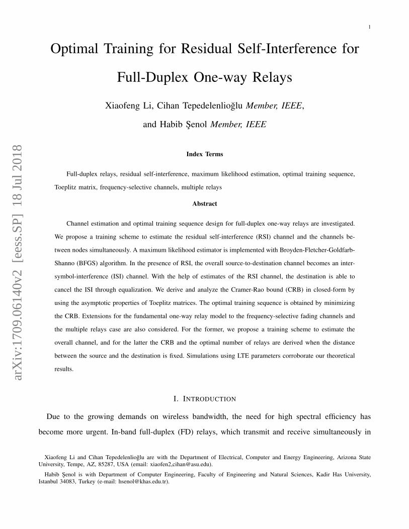
Fig. 6. BER comparison of different detectors. Fig. 7. MSE with increasing N in frequency-selective case.

also two cases for MF detector. In one case, MF detector is directly used to the received signal which

has colored noise. The other case is obtained by first applying a noise whitening filter to the received

signal and then doing MF detection. So the noise is whitened in this case. From the perspective of how

much CSI is needed, the former case only needs h while the latter needs both h and θ. Figure 6 shows

the Viterbi equalizer outperforms any MF detector since the equalizer cancels the RSI while MF treats

the RSI as noise. For the two MF detectors, the one that whitens the noise has better performance

which comes from the noise whitening filter by using the CSI of θ. The fact that canceling the RSI and

whitening the noise lead to better performance illustrates the benefits of estimating the RSI channel

θ.

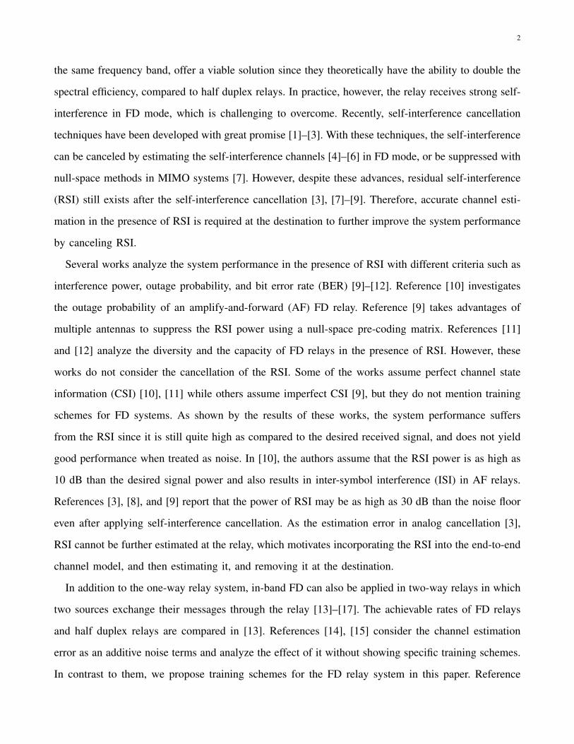
Figures 7 and 8 show the MSE of the two extensions. Note that the estimator are derived by

using H f in (49) and H(1) in (58) which are the approximation of the exact channels for frequency-

selective case and multi-relay case respectively. The MSE is calculated by comparing the estimates

of the approximation to the exact channels. Figure 7 shows that in the frequency-selective case, the

MSE reduces with the training length N increasing, implying that the asymptotic approximation H f

gets closer to the exact channels. The reducing MSE shows the accuracy of the approximation.

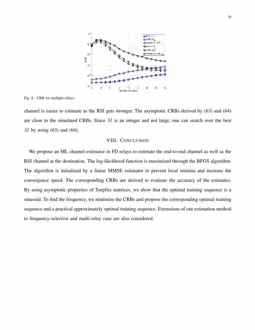
Figure 8 shows the MSEs of zM and h(1)2 compared with their CRBs in the multi-relay case.

Specifically, the total path loss between the source and the relay is K = −60 dB and path-loss

exponent is γ = 3.71 for the outdoor environment. As M increases, the MSE of zM increases because

more noise and interference are added. On the other hand, the MSE of h(1)2 decreases, since the RSI

26

Fig. 8. CRB for multiple relays.

channel is easier to estimate as the RSI gets stronger. The asymptotic CRBs derived by (63) and (64)

are close to the simulated CRBs. Since M is an integer and not large, one can search over the best

M by using (63) and (64).

VIII. CONCLUSION

We propose an ML channel estimator in FD relays to estimate the end-to-end channel as well as the

RSI channel at the destination. The log-likelihood function is maximized through the BFGS algorithm.

The algorithm is initialized by a linear MMSE estimator to prevent local minima and increase the

convergence speed. The corresponding CRBs are derived to evaluate the accuracy of the estimates.

By using asymptotic properties of Toeplitz matrices, we show that the optimal training sequence is a

sinusoid. To find the frequency, we minimize the CRBs and propose the corresponding optimal training

sequence and a practical approximately optimal training sequence. Extensions of our estimation method

to frequency-selective and multi-relay case are also considered.

27

APPENDIX I

MEAN AND COVARIANCE MATRIX OF p(y|h, θ)

In (5), h and θ are parameters of interest and d is the nuisance parameter. The likelihood function

p(y|h, θ) is obtained through integrating p(y|h, θ, d) with respect to d [30],

p(y|h, θ) =

∫p(y|h, θ, d)p(d)dd. (65)

Since p(y|h, θ, d) and p(d) are Gaussian distributed, it can be shown that the distribution of p(y|h, θ)

is also Gaussian. Denoting the mean of y given h and θ to be E[y|h, θ] and the covariance matrix as

V [y|h, θ]. It can be shown that

E[y|h, θ] = Ed[Ey[y|h, θ, d]], V [y|h, θ] = Vd[Ey[y|h, θ, d]] + Ed[Vy[y|h, θ, d]]. (66)

Since we know p(y|h, θ, d) is a Gaussian distribution with mean µ and co-variance matrix C, then it

is straight forward to get

Ey[y|h, θ, d] = hHθ, Vy[y|h, θ, d] = |d|2σ2rHθH

Hθ + σ2

dIN . (67)

The distribution of p(d) is also Gaussian with zero mean and variance α2, thus

Ed[Ey[y|h, θ, d]] = Ed[hHθ] = hHθ, Vd[Ey[y|h, θ, d]] = Vd[hHθ] = 0N×N , (68)

Ed[Vy[y|h, θ, d]] = Ed[|d|2σ2rHθH

Hθ + σ2

dIN ] = α2σ2rHθH

Hθ + σ2

dIN . (69)

Therefore, we can obtain the mean and covariance matrix of the Gaussian distribution p(y|h, θ),

µ = E[y|h, θ] = hHθ, C = V [y|h, θ] = α2σ2rHθH

Hθ + σ2

dIN . (70)

APPENDIX II

UNKNOWN DELAY τ0 AT THE RELAY

We first begin considering our discrete signal model under unknown τ0 ∈ R+. When the desired

received signal and the RSI signal are not synchronized, we jointly estimate τ0 and the channels.

Assume that the analog transmitted signal, the received signal at the relay, and the received signal

28

at the destination are x(t), yr(t), and yd(t) respectively. The source-relay, relay-destination, and RSI

channels are hsr(τ) = hsrδ(τ), hrd(τ) = hrdδ(τ) and hrr(τ) = θδ(τ) where hsr, hrd and θ are the

channel coefficients and the variable τ is the delay of the channels. The three channels are assumed

to be time-invariant and flat fading. Let s[n] be the sequence that the source transmitted. The source

transmit signal is x(t) =∑+∞

n=−∞ s[n]ptr(t − nTs) where Ts is the symbol duration and ptr(t) is a

pulse shaping filter. The relay forwards the superimposed signal of the desired received signal and the

RSI signal to the destination. By ignoring the noise, we have

yr(t) = (hsr ∗ x)(t) + (hrr ∗ yr)(t− τ0), yd(t) = (hrd ∗ yr ∗ prec)(t), (71)

where prec(t) is the matched filter at the destination. The notation ∗ stands for convolution. The delayed

version of yr(t) is yr(t − τ0) = (hsr ∗ x)(t − τ0) + (hrr ∗ yr)(t − 2τ0). By substituting yr(t − τ0) and

x(t) into yd(t), we have

yd(t) = h+∞∑

n=−∞

s[n]

(L−1∑l=0

θlp(t− nTs − lτ0)

)(72)

where L is the effective length of the overall channel impulse response, |θ|L ≈ 0 by the finite energy

assumption, coefficient h = hrdhsr, and p(t) = ptr(t)∗prec(t) is a raised-cosine filter. At the destination,

we sample the received signal with the same sampling rate 1/Ts. The sampled signal is

yd(kTs) = h+∞∑

n=−∞

s[n]

(L−1∑l=0

θlp(kTs − nTs − lτ0)

). (73)

We can obtain a discrete signal model

yd(kTs) = yd[k] = s[n] ∗ h[k − n], (74)

where

h[k] =L−1∑l=0

hθlp(kTs − lτ0) , hg[k]. (75)

Note that since τ0 is not an integer multiple of Ts, the delayed signal and the source-relay signal

are not synchronized. The sampling point of the overlapped signal of the two signals is not exactly

the zero positions of the raised-cosine filter. Therefore, the resulting discrete-time channel model has

non-zero coefficients given by (75). Define an N by N Toeplitz matrix as H [a] whose first column is

29

[a[0], a[1], · · · , a[M − 1], 0, · · · , 0]T and first row is [a[0], 0, · · · , 0] where a = [a[0], a[1], · · · , a[M ]]T ,

M ≤ N . Therefore, the channel matrix is hH [g] with g = [g[0], g[1], · · · , g[N − 1]]T . The destination

received signal in vector form is

y = hH [g]x+ dH [g]nr + nd. (76)

ML estimator: We can find the mean and covariance matrix of y as

µ = hH [g], C = α2σ2rH [g]HH [g] + σ2

dIN . (77)

The ML estimator is given by

h, θ, τ0 = arg minh,θ,τ0

log |C|+ (y − µ)HC−1(y − µ)

. (78)

We can eliminate h and find the derivatives of the log-likelihood function with respect to θ by the

same way as the case with known τ0. For the unknown τ0, we need to find the derivatives of the

log-likelihood function with respect to it as follows.

Define b[k] and q[k] as the derivatives of g[k] with respect to θ and τ0 respectively,

b[k] =L−1∑l=0

lθl−1p(kTs − lτ0), q[k] = −L−1∑l=0

lθlp′(kTs − lτ0) (79)

where p′(t) is the derivative of p(t). The derivative of C with respect to τ0 is

Bτ0 =∂C

∂τ0

= α2σ2r

(H [g]HH [q] +HH [g]H [q]

). (80)

Therefore, we have

∂f

∂τ0

= −tr(C−1Bτ0

)+ (y − µ)HC−1Bτ0C

−1(y − µ) + 2Re[(y − µ)HC−1hH [q]x

]. (81)

With the gradients of τ0 and θ, the ML estimator can be solved by the BFGS algorithm.

CRBs: Let ξ = [h θ τ0]T be the vector of unknown parameters. The Fisher information of the

parameters is given by the following.

30

Γ11 = xHHH [g]C−1H [g]x, (82)

Γ22 = |h|2xHHH [b]C−1H [b]x+ α4σ4r tr(C−1H [g]HH [b]C−1H [b]HH [g]

), (83)

Γ33 = |h|2xHHH [q]C−1H [q]x+ tr(C−1Bτ0C

−1Bτ0

). (84)

Similarly, Γ12, Γ13, and Γ23 can be found. The CRBs are given by the trace of the inverse of the Fisher

information matrix.

Updated asymptotic CRB analysis: Next we explain how to update our CRB analysis with un-

known τ0. The key idea in the analysis is that the Toeplitz channel matrix behaves as a circulant matrix

asymptotically when the size of it goes to infinity and we can find the eigenvalues and corresponding

eigenvectors through function t(λ) which characterizes the asymptotic circulant matrix. To modify the

analysis, we need to find a new function tτ0(λ) =∑+∞

k=−∞ h[k]ejλk which is a discrete-time Fourier

transform (DTFT) of h[k] in closed-form. When the delay lτ0 in h[k] is not an integer multiple of

Ts, the DTFT with a time shift cannot be applied directly. We use the relationship of the continuous

signal hc(t) of which h[n] are the samples, the impulse train hp(t) with amplitudes corresponding to

the samples of hc(t), and the discrete samples h[n] [34]. We can find the DTFT of h[n] as

Hd(ejΩ) =1

Ts

L−1∑l=0

hθlPc (jΩ/Ts) e−jΩlτ0/Ts , (85)

where Pc(jω) is the continuous Fourier transform of hc(t), Ω is the frequency variable with period

2π/Ts. We have tτ0(λ) = Hd(ejλ). Therefore, our CRB analysis based on the closed-form expression

of t(λ) also works for tτ0(λ).

APPENDIX III

THE GRADIENTS USED IN THE BFGS ALGORITHM

Now we derive the gradients of f with respect to θx and θy which are used in the BFGS algorithm.

The gradients for both real and imaginary parts are needed as inputs of the algorithm. For θ, we first

obtain the derivative of Hθ with respect to θ, denoted as Bθ, which is also an N ×N Toeplitz matrix

with first column [0, 1, 2θ, · · · , (L− 1)θL−2, 0, · · · , 0]T and first row 0TN×1.

31

Both C and µ contain θ, therefore there are three terms in its gradient. We have

∇fθx = tr(α2σ2

rC−1(BθH

Hθ +HθB

Hθ ))− 2Re

[(y − µ)HC−1hBθx

]− α2σ2

r (y − µ)HC−1(BθHHθ +HθB

Hθ )C−1(y − µ), (86)

∇fθy = tr(jα2σ2

rC−1(BθH

Hθ −HθB

Hθ ))− 2Re

[(y − µ)HC−1jhBθx

]− jα2σ2

r (y − µ)HC−1(BθHHθ −HθB

Hθ )C−1(y − µ). (87)

REFERENCES

[1] M. Heino, D. Korpi, T. Huusari, E. Antonio-Rodriguez, S. Venkatasubramanian, T. Riihonen, L. Anttila, C. Icheln, K. Haneda,

and R. Wichman, “Recent advances in antenna design and interference cancellation algorithms for in-band full duplex relays,”

IEEE Communications Magazine, vol. 53, no. 5, pp. 91–101, Oct. 2015.

[2] S.-K. Hong, J. Brand, J. Choi, M. Jain, J. Mehlman, S. Katti, and P. Levis, “Applications of self-interference cancellation in 5G

and beyond,” IEEE Communications Magazine, vol. 52, no. 2, pp. 114–121, Oct. 2014.

[3] A. Sabharwal, P. Schniter, D. Guo, D. W. Bliss, S. Rangarajan, and R. Wichman, “In-band full-duplex wireless: Challenges and

opportunities,” IEEE Journal on Selected Areas in Communications, vol. 32, no. 9, pp. 1637–1652, Sep. 2014.

[4] J. Ma, G. Y. Li, J. Zhang, T. Kuze, and H. Iura, “A new coupling channel estimator for cross-talk cancellation at wireless relay

stations,” in Proc. IEEE Global Telecommun. Conf., Oct. 2009, pp. 1–6.

[5] A. Masmoudi and T. Le-Ngoc, “A maximum-likelihood channel estimator for self-interference cancellation in full-duplex systems,”

IEEE Transactions on Vehicular Technology, vol. 65, no. 7, pp. 5122–5132, Oct. 2016.

[6] A. Koohian, H. Mehrpouyan, M. Ahmadian, and M. Azarbad, “Bandwidth efficient channel estimation for full duplex communi-

cation systems,” in Proc. IEEE ICC, Oct. 2015, pp. 4710–4714.

[7] T. Riihonen, S. Werner, and R. Wichman, “Mitigation of loopback self-interference in full-duplex MIMO relays,” IEEE Transactions

on Signal Processing, vol. 59, no. 12, pp. 5983–5993, Dec. 2011.

[8] M. Duarte, C. Dick, and A. Sabharwal, “Experiment-driven characterization of full-duplex wireless systems,” IEEE Transactions

on Wireless Communications, vol. 11, no. 12, pp. 4296–4307, Dec. 2012.

[9] T. Riihonen, S. Werner, and R. Wichman, “Residual self-interference in full-duplex MIMO relays after null-space projection and

cancellation,” in Proc. IEEE 44th Asilomar Conf. Signals, Syst. Comput., Nov. 2010, pp. 653–657.

[10] T. M. Kim and A. Paulraj, “Outage probability of amplify-and-forward cooperation with full duplex relay,” in Proc. IEEE WCNC,

Oct. 2012, pp. 75–79.

[11] L. Jimenez Rodriguez, N. H. Tran, and T. Le-Ngoc, “Performance of full-duplex af relaying in the presence of residual self-

interference,” IEEE Journal on Selected Areas in Communications, vol. 32, no. 9, pp. 1752–1764, Jun. 2014.

[12] ——, “Optimal power allocation and capacity of full-duplex af relaying under residual self-interference,” IEEE Wireless

Communications Letters, vol. 3, no. 2, pp. 233–236, Apr. 2014.

[13] X. Cheng, B. Yu, X. Cheng, and L. Yang, “Two-way full-duplex amplify-and-forward relaying,” in Proc. IEEE Military Commun.

Conf., Oct. 2013, pp. 1–6.

32

[14] F. S. Tabataba, P. Sadeghi, C. Hucher, and M. R. Pakravan, “Impact of channel estimation errors and power allocation on analog

network coding and routing in two-way relaying,” IEEE Transactions on Vehicular Technology, vol. 61, no. 7, pp. 3223–3239,

Oct. 2012.

[15] D. Kim, H. Ju, S. Park, and D. Hong, “Effects of channel estimation error on full-duplex two-way networks,” IEEE Transactions

on Vehicular Technology, vol. 62, no. 9, pp. 4666–4672, Oct. 2013.

[16] G. Zheng, “Joint beamforming optimization and power control for full-duplex MIMO two-way relay channel,” IEEE Transactions

on Signal Processing, vol. 63, no. 3, pp. 555–566, Oct. 2015.

[17] X. Li, C. Tepedelenlioglu, and H. Senol, “Channel estimation for residual self-interference in full duplex amplify-and-forward

two-way relays,” IEEE Transactions on Wireless Communications, vol. 16, no. 8, pp. 4970–4983, Oct. 2017.

[18] M. Mohammadi, B. K. Chalise, H. A. Suraweera, C. Zhong, G. Zheng, and I. Krikidis, “Throughput analysis and optimization

of wireless-powered multiple antenna full-duplex relay systems,” IEEE Transactions on Communications, vol. 64, no. 4, pp.

1769–1785, Oct. 2016.

[19] J. S. Lemos, F. A. Monteiro, I. Sousa, and A. Rodrigues, “Full-duplex relaying in MIMO-OFDM frequency-selective channels

with optimal adaptive filtering,” in Proc. IEEE Global Conf. on Signal and Inf. Process., Oct. 2015, pp. 1081–1085.

[20] A. C. Cirik, M. C. Filippou, and T. Ratnarajaht, “Transceiver design in full-duplex MIMO cognitive radios under channel

uncertainties,” IEEE Transactions on Cognitive Communications and Networking, vol. 2, no. 1, pp. 1–14, Oct. 2016.

[21] B. P. Day, A. R. Margetts, D. W. Bliss, and P. Schniter, “Full-duplex MIMO relaying: Achievable rates under limited dynamic

range,” IEEE Journal on Selected Areas in Communications, vol. 30, no. 8, pp. 1541–1553, Sep. 2012.

[22] ——, “Full-duplex bidirectional MIMO: Achievable rates under limited dynamic range,” IEEE Transactions on Signal Processing,

vol. 60, no. 7, pp. 3702–3713, Jul. 2012.

[23] O. Taghizadeh, M. Rothe, A. C. Cirik, and R. Mathar, “Distortion-loop analysis for full-duplex amplify-and-forward relaying in

cooperative multicast scenarios,” in Proc. IEEE Int. Conf. Signal Process. and Commun. Syst., Oct. 2015, pp. 1–9.

[24] O. Taghizadeh, T. Yang, A. C. Cirik, and R. Mathar, “Distortion-loop-aware amplify-and-forward full-duplex relaying with multiple

antennas,” in Proc. IEEE Int. Symp. Wireless Commun. Syst., Oct. 2016, pp. 54–58.

[25] H. Q. Ngo, H. A. Suraweera, M. Matthaiou, and E. G. Larsson, “Multipair full-duplex relaying with massive arrays and linear

processing,” IEEE Journal on Selected Areas in Communications, vol. 32, no. 9, pp. 1721–1737, Oct. 2014.

[26] X. Xiong, X. Wang, T. Riihonen, and X. You, “Channel estimation for full-duplex relay systems with large-scale antenna arrays,”

IEEE Transactions on Wireless Communications, vol. 15, no. 10, pp. 6925–6938, Oct. 2016.

[27] X. Li and C. Tepedelenlioglu, “Maximum likelihood channel estimation for residual self-interference cancellation in full duplex

relay,” in Proc. IEEE 49th Asilomar Conf. Signals, Syst. Comput., Nov. 2015, pp. 807–811.

[28] J. B. Calvert. Analog delay devices. [Online]. Available: http://mysite.du.edu/∼etuttle/electron/elect39.htm

[29] T. Riihonen, S. Werner, and R. Wichman, “Optimized gain control for single-frequency relaying with loop interference,” IEEE

Transactions on Wireless Communications, vol. 8, no. 6, pp. 2801–2806, Oct. 2009.

[30] S. M. Kay, Fundamentals of Statistical Signal Processing: Estimation Theory. Englewood Cliffs, NJ, USA: Prentice-Hall, 1993.

[31] K. P. Murphy, Machine Learning: A Probabilistic Perspective. Cambridge, MA, USA: MIT Press, 2012.

[32] R. M. Gray, Toeplitz and Circulant Matrices: A Review. LP Breda, The Netherlands: Now Publishers, Oct. 2006.

[33] A. Goldsmith, Wireless Communications. New York, NY, USA: Cambridge University Press, 2005.

[34] A. Oppenheim, A. Willsky, and S. Nawab, Signals and Systems. New Jersey, NJ, USA: Prentice Hall, 1997.