1

Online (Recursive) Robust Principal Components AnalysisNamrata Vaswani, Chenlu Qiu, Brian Lois, Han Guo and Jinchun Zhan

Iowa State University, Ames IA, USAEmail: namrata@iastate.edu

Abstract

This work studies the problem of sequentially recovering a sparse vector St and a vector from a low-dimensional subspaceLt from knowledge of their sum Mt := Lt + St. If the primary goal is to recover the low-dimensional subspace in which theLt’s lie, then the problem is one of online or recursive robust principal components analysis (PCA). An example of where such aproblem might arise is in separating a sparse foreground and a slowly changing dense background in a surveillance video. In thischapter, we describe our recently proposed algorithm, called Recursive Projected Compressed Sensing (ReProCS), to solve thisproblem and demonstrate its significant advantage over other robust PCA based methods for this video layering problem. We alsosummarize the performance guarantees for ReProCS. Lastly, we briefly describe our work on modified-PCP, which is a piecewisebatch approach that removes a key limitation of ReProCS, however it retains a key limitation of existing work.

I. INTRODUCTION

Principal Components Analysis (PCA) is a widely used dimension reduction technique that finds a small number of orthogonalbasis vectors, called principal components, along which most of the variability of the dataset lies. It is well known that PCAis sensitive to outliers. Accurately computing the principal subspace in the presence of outliers is called robust PCA [?],[?], [?], [?]. Often, for time series data, the principal subspace changes gradually over time. Updating its estimate on-the-fly(recursively) in the presence of outliers, as more data comes in is referred to as online or recursive robust PCA [?], [?], [?].“Outlier” is a loosely defined term that refers to any corruption that is not small compared to the true data vector and thatoccurs occasionally. As suggested in [?], [?], an outlier can be nicely modeled as a sparse vector whose nonzero values canhave any magnitude.

A key application where the robust PCA problem occurs is in video analysis where the goal is to separate a slowly changingbackground from moving foreground objects [?], [?]. If we stack each frame as a column vector, the background is wellmodeled as being dense and lying in a low dimensional subspace that may gradually change over time, while the movingforeground objects constitute the sparse outliers [?], [?]. Other applications include detection of brain activation patterns fromfunctional MRI (fMRI) sequences (the “active” part of the brain can be interpreted as a sparse outlier), detection of anomalousbehavior in dynamic social networks and sensor networks based detection and tracking of abnormal events such as forest firesor oil spills. In most of these applications, an online solution is desirable.

The moving objects or the active regions of the brain or the oil spill region may be “outliers” for the PCA problem, but inmost cases, these are actually the signals-of-interest whereas the background image is the noise. Also, all the above signals-of-interest are sparse vectors. Thus, this problem can also be interpreted as one of recursively recovering a time sequenceof sparse signals, St, from measurements Mt := St + Lt that are corrupted by (potentially) large magnitude but dense andstructured noise, Lt. The structure that we require is that Lt be dense and lie in a low dimensional subspace that is eitherfixed or changes “slowly enough”.

A. Related Work

There has been a large amount of work on robust PCA, e.g. [?], [?], [?], [?], [?], [?], [?], and recursive or online orincremental robust PCA e.g. [?], [?], [?]. In most of these works, either the locations of the missing/corruped data points areassumed known [?] (not a practical assumption); or they first detect the corrupted data points and then replace their valuesusing nearby values [?]; or weight each data point in proportion to its reliability (thus soft-detecting and down-weighting thelikely outliers) [?], [?]; or just remove the entire outlier vector [?], [?]. Detecting or soft-detecting outliers (St) as in [?], [?],[?] is easy when the outlier magnitude is large, but not otherwise. When the signal of interest is St, the most difficult situationis when nonzero elements of St have small magnitude compared to those of Lt and in this case, these approaches do not work.

In recent works [?], [?], a new and elegant solution to robust PCA called Principal Components’ Pursuit (PCP) has beenproposed, that does not require a two step outlier location detection/correction process and also does not throw out the entirevector. It redefines batch robust PCA as a problem of separating a low rank matrix, Lt := [L1, . . . , Lt], from a sparse matrix,St := [S1, . . . , St], using the measurement matrix, Mt := [M1, . . . ,Mt] = Lt + St.

2

Let ‖A‖∗ be the nuclear norm of A (sum of singular values of A) while ‖A‖1 is the `1 norm of A seen as a long vector.It was shown in [?] that, with high probability (w.h.p.), one can recover Lt and St exactly by solving PCP:

minL,S‖L‖∗ + λ‖S‖1 subject to L+ S =Mt (1)

provided that (a) the left and right singular vectors of Lt are dense; (b) any element of the matrix St is nonzero w.p. %, andzero w.p. 1− %, independent of all others; and (c) the rank of Lt and the support size of St are bounded by a small enoughvalues.

B. Our work: provably correct and practically usable recursive robust PCA solutions

As described earlier, many applications where robust PCA is required, such as video surveillance, require an online (recursive)solution. Even for offline applications, a recursive solution is typically faster than a batch one. Moreover, in many of theseapplications, the support of the sparse part changes in a correlated fashion over time, e.g., in video foreground objects donot move randomly, and may also be static for short periods of time. In recent work [?], [?], [?], [?], we introduced a novelsolution approach, called Recursive Projected Compressive Sensing (ReProCS), that recursively recovered St and Lt at eachtime t. Moreover, as we showed later in [?], [?], it can also provably handle correlated support changes significantly betterthan batch approaches because it uses extra assumptions (accurate initial subspace knowledge and slow subspace change).In simulation and real data experiments (see [?] and http://www.ece.iastate.edu/∼chenlu/ReProCS/ReProCS main.htm), it wasfaster than batch methods such as PCP and also significantly outperformed them in situations where the support changes werecorrelated over time (as long as there was some support change every few frames). In [?], we studied a simple modificationof the original ReProCS idea and obtained a performance guarantee for it. This result needed mild assumptions except one: itneeded an assumption on intermediate algorithm estimates and hence it was not a correctness result. In very recent work [?],[?], we also have a complete correctness result for ReProCS that replaces this restrictive assumption by a simple and practicalassumption on support change of St.

The ReProCS algorithm itself has a key limitation that is removed by our later work on modified-PCP [?], [?] (see Section??), however as explained in Sec ??, modified-PCP does not handle correlated support change as well as ReProCS. In thisbookchapter we provide an overview of both ReProCS and modified-PCP and a discussion of when which is better and why.We briefly also explain their correctness results and show simulation and real data experiments comparing them with variousexisting batch and online robust PCA solutions.

To the best of our knowledge, [?] provided the first performance guarantee for an online robust PCA approach or equivalentlyfor an online sparse + low-rank matrix recovery approach. Of course it was only a partial result (depended on intermediatealgorithm estimates satisfying a certain property). Another partial result for online robust PCA was given in more recent workby Feng et al [?]. In very recent work [?], [?], we provide the first complete correctness result for an online robust PCA /online sparse + low-rank matrix recovery approach. Another online algorithm that addresses the online robust PCA problem isGRASTA [?], however, it does not contain any performance analysis. We should mention here that our results directly applyto the recursive version of the matrix completion problem [?] as well since it is a simpler special case of the current problem(the support set of St is the set of indices of the missing entries and is thus known) [?]. We explicitly give the algorithm andresult for online MC in [?].

The proof techniques used in our work are very different from those used to analyze other recent batch robust PCA works[?], [?], [?], [?], [?], [?], [?], [?], [?], [?], [?], [?]. The works of [?], [?] also study a different case: that where an entire vectoris either an outlier or an inlier. Our proof utilizes (a) sparse recovery results [?]; (b) results from matrix perturbation theory thatbound the estimation error in computing the eigenvectors of a perturbed Hermitian matrix with respect to eigenvectors of theoriginal Hermitian matrix (the famous sin θ theorem of Davis and Kahan [?]) and (c) high probability bounds on eigenvaluesof sums of independent random matrices (matrix Hoeffding inequality [?]).

A key difference of our approach to analyzing the subspace estimation step compared with most existing work analyzingfinite sample PCA, e.g. [?] and references therein, is that it needs to provably work in the presence of error/noise that iscorrelated with Lt. Most existing works, including [?] and the references it discusses, assume that the noise is independentof (or at least uncorrelated with) the data. However, in our case, because of how the estimate Lt is computed, the erroret := Lt − Lt is correlated with Lt. As a result, the tools developed in these earlier works cannot be used for our problem.This is also the reason why simple PCA cannot be used and we need to develop and analyze a projection-PCA algorithm forsubspace tracking (this fact is explained in detail in the Appendix of [?]).

The ReProCS approach is related to that of [?], [?], [?] in that all of these first try to nullify the low dimensional signalby projecting the measurement vector into a subspace perpendicular to that of the low dimensional signal, and then solve

3

for the sparse “error” vector (outlier). However, the big difference is that in all of these works the basis for the subspaceof the low dimensional signal is perfectly known. Our work studies the case where the subspace is not known. We have aninitial approximate estimate of the subspace, but over time it can change significantly. In this work, to keep things simple,we mostly use `1 minimization done separately for each time instant (also referred to as basis pursuit denoising (BPDN))[?], [?]. However, this can be replaced by any other sparse recovery algorithm, either recursive or batch, as long as the batchalgorithm is applied to α frames at a time, e.g. one can replace BPDN by modified-CS or support-predicted modified-CS [?].We have used a combination of simple `1 minimization and modified-CS / weighted `1 in the practical version of the ReProCSalgorithm that was used for our video experiments (see Section ??).

C. Chapter Organization

This chapter is organized as follows. In Section ??, we give the problem definition and the key assumptions required. Weexplain the main idea of the ReProCS algorithm and develop its practically usable version in Section ??. We develop themodified-PCP solution in Section ??. The performance guarantees for both ReProCS and modified-PCP are summarized inSection ??. Numerical experiments, both for simulated data and for real video sequences, are shown in Section ??. Conclusionsand future work are discussed in Section ??.

D. Notation

For a set T ⊂ 1, 2, . . . , n, we use |T | to denote its cardinality, i.e., the number of elements in T . We use T c to denoteits complement w.r.t. 1, 2, . . . n, i.e. T c := i ∈ 1, 2, . . . n : i /∈ T .

We use the interval notation, [t1, t2], to denote the set of all integers between and including t1 to t2, i.e. [t1, t2] :=

t1, t1 + 1, . . . , t2. For a vector v, vi denotes the ith entry of v and vT denotes a vector consisting of the entries of v indexedby T . We use ‖v‖p to denote the `p norm of v. The support of v, supp(v), is the set of indices at which v is nonzero,supp(v) := i : vi 6= 0. We say that v is s-sparse if |supp(v)| ≤ s.

For a matrix B, B′ denotes its transpose, and B† its pseudo-inverse. For a matrix with linearly independent columns,B† = (B′B)−1B′. We use ‖B‖2 := maxx 6=0 ‖Bx‖2/‖x‖2 to denote the induced 2-norm of the matrix. Also, ‖B‖∗ is thenuclear norm (sum of singular values) and ‖B‖max denotes the maximum over the absolute values of all its entries. We letσi(B) denotes the ith largest singular value of B. For a Hermitian matrix, B, we use the notation B EVD

= UΛU ′ to denote theeigenvalue decomposition of B. Here U is an orthonormal matrix and Λ is a diagonal matrix with entries arranged in decreasingorder. Also, we use λi(B) to denote the ith largest eigenvalue of a Hermitian matrix B and we use λmax(B) and λmin(B) denoteits maximum and minimum eigenvalues. If B is Hermitian positive semi-definite (p.s.d.), then λi(B) = σi(B). For Hermitianmatrices B1 and B2, the notation B1 B2 means that B2−B1 is p.s.d. Similarly, B1 B2 means that B1−B2 is p.s.d. Fora Hermitian matrix B, ‖B‖2 =

√max(λ2

max(B), λ2min(B)) and thus, ‖B‖2 ≤ b implies that −b ≤ λmin(B) ≤ λmax(B) ≤ b.

We use the notation B SV D= UΣV ′ to denote the singular value decomposition (SVD) of B with the diagonal entries of Σ

being arranged in non-decreasing order.We use I to denote an identity matrix of appropriate size. For an index set T and a matrix B, BT is the sub-matrix of B

containing columns with indices in the set T . Notice that BT = BIT . Given a matrix B of size m×n and B2 of size m×n2,[B B2] constructs a new matrix by concatenating matrices B and B2 in the horizontal direction. Let Brem be a matrix formedby some columns of B. Then B \Brem is the matrix B with columns in Brem removed.

The notation [.] denotes an empty matrix.For a matrix M ,• span(M) denotes the subspace spanned by the columns of M .• M is a basis matrix if M ′M = I .• The notation Q = basis(span(M)), or Q = basis(M) for short, means that Q is a basis matrix for span(M) i.e. Q

satisfies Q′Q = I and span(Q) = span(M).• The b% left singular values’ set of a matrix M is the smallest set of indices of its singular values that contains at

least b% of the total singular values’ energy. In other words, if M SV D= UΣV ′, it is the smallest set T such that∑

i∈T (Σ)2i,i ≥ b

100

∑ni=1(Σ)2

i,i.• The corresponding matrix of left singular vectors, UT , is referred to as the b% left singular vectors’ matrix.• The notation [Q,Σ] = approx-basis(M, b%) means that Q is the b% left singular vectors’ matrix for M and Σ is the

diagonal matrix with diagonal entries equal to the b% left singular values’ set.• The notation Q = approx-basis(M, r) means that Q contains the left singular vectors of M corresponding to its r largest

singular values. This is also sometimes referred to as: Q contains the r top singular vectors of M .

4

Definition 1.1. The s-restricted isometry constant (RIC) [?], δs, for an n×m matrix Ψ is the smallest real number satisfying(1− δs)‖x‖22 ≤ ‖ΨTx‖22 ≤ (1 + δs)‖x‖22 for all sets T with |T | ≤ s and all real vectors x of length |T |.

II. PROBLEM DEFINITION AND MODEL ASSUMPTIONS

We give the problem definition below followed by the model and then describe the key assumptions needed.

A. Problem Definition

The measurement vector at time t, Mt, is an n dimensional vector which can be decomposed as

Mt = Lt + St (2)

Here St is a sparse vector with support set size at most s and minimum magnitude of nonzero values at least Smin. Lt is adense but low dimensional vector, i.e. Lt = P(t)at where P(t) is an n × r(t) basis matrix with r(t) < n, that changes everyso often according to the model given below. We are given an accurate estimate of the subspace in which the initial ttrain

Lt’s lie, i.e. we are given a basis matrix P0 so that ‖(I − P0P′0)P0‖2 is small. Here P0 is a basis matrix for span(Lttrain), i.e.

span(P0) = span(Lttrain). Also, for the first ttrain time instants, St is zero. The goal is

1) to estimate both St and Lt at each time t > ttrain, and2) to estimate span(Lt) every so often, i.e. compute P(t) so that the subspace estimation error, SE(t) := ‖(I−P(t)P

′(t))P(t)‖2

is small.

We assume a subspace change model that allows the subspace to change at certain change times tj rather than continuouslyat each time. It should be noted that this is only a model for reality. In practice there will typically be some changes at everytime t; however this is difficult to model in a simple fashion. Moreover the analysis for such a model will be a lot morecomplicated. However, we do allow the variance of the projection of Lt along the subspace directions to change continuously.The projection along the new directions is assumed to be small initially and allowed to gradually increase to a large value (seeSec ??).

Model 2.1 (Model on Lt).1) We assume that Lt = P(t)at with P(t) = Pj for all tj ≤ t < tj+1, j = 0, 1, 2 · · · J . Here Pj is an n × rj basis matrix

with rj < min(n, (tj+1 − tj)) that changes as

Pj = [Pj−1 Pj,new]

where Pj,new is a n× cj,new basis matrix with P ′j,newPj−1 = 0. Thus

rj = rank(Pj) = rj−1 + cj,new.

We let t0 = 0. Also tJ+1 = tmax which is the length of the sequence. This can be infinite too. This model is illustratedin Figure ??.

2) The vector of coefficients, at := P(t)′Lt, is a zero mean random variable (r.v.) with mutually uncorrelated entries, i.e.

E[at] = 0 and Λt := Cov[at] = E(ata′t) is a diagonal matrix. This assumption follows automatically if we let P(t)ΛtP(t)

′

be the eigenvalue decomposition (EVD) of Cov(Lt). .3) Assume that 0 < λ− ≤ λ+ <∞ where

λ− := inftλmin(Λt), λ+ := sup

tλmax(Λt)

Notice that, for tj ≤ t < tj+1, at is an rj length vector which can be split as

at = Pj′Lt =

[at,∗at,new

]where at,∗ := Pj−1

′Lt and at,new := Pj,new′Lt. Thus, for this interval, Lt can be rewritten as

Lt = [Pj−1 Pj,new]

[at,∗at,new

]= Pj−1at,∗ + Pj,newat,new

Also, Λt can be split as

Λt =

[Λt,∗ 0

0 Λt,new

]

5

Fig. 1. The subspace change model explained in Sec ??. Here t0 = 0 and 0 < ttrain < t1.

where Λt,∗ = Cov[at,∗] and Λt,new = Cov[at,new] are diagonal matrices.

Definition 2.2. Define

f :=λ+

λ−

Define

λ−new := mintλmin(Λt,new), λ+

new := maxtλmax(Λt,new), g :=

λ+new

λ−new

Notice that the set of new directions changes with each subspace change interval and hence at any time g is an upper boundon the condition number of Λt,new for the currrent set of new directions.

The above simple model only allows new additions to the subspace and hence the rank of Pj can only grow over time. TheReProCS algorithm designed for this model can be interpreted as a recursive algorithm for solving the robust PCA problemstudied in [?] and other batch robust PCA works. At time t we estimate the subspace spanned by L1, L2, . . . Lt. We give thismodel first for ease of understanding. Both our algorithm and its guarantee will apply without any change even if one or moredirections were deleted from the subspace with the following more general model.

Model 2.3. Assume Model ?? with the difference that Pj now changes as

Pj = [(Pj−1Rj \ Pj,old) Pj,new]

where Pj,new is a n × cj,new basis matrix with P ′j,newPj−1 = 0, Rj is a rotation matrix and Pj,old is a n × cj,old matrixcontaining columns of (Pj−1Rj).

B. Slow subspace change

By slow subspace change we mean all of the following.First, the delay between consecutive subspace change times is large enough, i.e., for a d large enough,

tj+1 − tj ≥ d (3)

Second, the magnitude of the projection of Lt along the newly added directions, at,new, is initially small but can increasegradually. We model this as follows. Assume that

λ+new ≤ g+λ−new (4)

for a g+ ≥ 1 but not too large; and for an α > 0 1 the following holds

‖at,new‖∞ ≤ min(vt−tjα −1γnew, γ∗

)(5)

when t ∈ [tj , tj+1 − 1] for a v ≥ 1 but not too large and with γnew < γ∗ and γnew < Smin. Clearly, the above assumptionimplies that

‖at,new‖∞ ≤ γnew,k := min(vk−1γnew, γ∗)

for all t ∈ [tj + (k − 1)α, tj + kα− 1].Third, the number of newly added directions is small, i.e. cj,new ≤ cmax r0.The last two assumptions are verified for real video data in [?, Section IX-A].

1As we will see in the algorithm α is the number of previous frames used to get a new estimate of Pj,new.

6

Remark 2.4 (Large f ). Since our problem definition allows large noise, Lt, but assumes slow subspace change, thus f =

λ+/λ− cannot be bounded by a small value. The reason is as follows. Slow subspace change implies that the projectionof Lt along the new directions is initially small, i.e. γnew is small. Since λ− ≤ γnew, this means that λ− is small. SinceE[‖Lt‖2] ≤ rmaxλ

+ and rmax is small (low-dimensional), thus, large Lt means that λ+ needs to be large. As a result fcannot be upper bounded by a small value.

C. Measuring denseness of a matrix and its relation with RIC

Before we can state the denseness assumption, we need to define the denseness coefficient.

Definition 2.5 (denseness coefficient). For a matrix or a vector B, define

κs(B) = κs(span(B)) := max|T |≤s

‖IT ′basis(B)‖2 (6)

where ‖.‖2 is the vector or matrix `2-norm.

Clearly, κs(B) ≤ 1. First consider an n-length vector B. Then κs measures the denseness (non-compressibility) of B. Asmall value indicates that the entries in B are spread out, i.e. it is a dense vector. A large value indicates that it is compressible(approximately or exactly sparse). The worst case (largest possible value) is κs(B) = 1 which indicates that B is an s-sparsevector. The best case is κs(B) =

√s/n and this will occur if each entry of B has the same magnitude. Similarly, for an n× r

matrix B, a small κs means that most (or all) of its columns are dense vectors.

Remark 2.6. The following facts should be noted about κs(.):

1) For a given matrix B, κs(B) is an non-decreasing function of s.2) κs([B1]) ≤ κs([B1 B2]) i.e. adding columns cannot decrease κs.3) A bound on κs(B) is κs(B) ≤

√sκ1(B). This follows because ‖B‖2 ≤

∥∥[‖b1‖2 . . . ‖br‖2]∥∥2where bi is the ith column

of B.4) For a basis matrix P = [P1, P2], κs([P1, P2])2 ≤ κs(P1)2 + κs(P2)2

The lemma below relates the denseness coefficient of a basis matrix P to the RIC of I−PP ′. The proof is in the Appendix.

Lemma 2.7. For an n× r basis matrix P (i.e P satisfying P ′P = I),

δs(I − PP ′) = κ2s(P ).

In other words, if the columns of P are dense enough (small κs), then the RIC of I − PP ′ is small.In this work, we assume an upper bound on κ2s(Pj) for all j, and a tighter upper bound on κ2s(Pj,new), i.e., there exist

κ+2s,∗ < 1 and a κ+

2s,new < κ+2s,∗ such that

maxjκ2s(Pj−1) ≤ κ+

2s,∗ and maxjκ2s(Pj,new) ≤ κ+

2s,new (7)

The denseness coefficient κs(B) is related to the denseness assumption required by PCP [?]. That work uses κ1(B) toquantify denseness. To relate to their condition, define the incoherence parameter µ as in [?] to be the smallest real numbersuch that

κ1(P0)2 ≤ µr0

nand κ1(Ptj ,new)2 ≤ µcj,new

nfor all j = 1, 2, . . . J (8)

Then, using Remark ??, it is easy to see that (??) holds if

2s(r0 + Jcmax)µ

n≤ κ+

2s,∗2

and2scmaxµ

n≤ κ+

2s,new

2(9)

where

cmax := maxjcj,new.

7

D. Definitions and assumptions on the sparse outliers

Define the following quantities for the sparse outliers.

Definition 2.8. Let Tt := i : (St)i 6= 0 denote the support set of St. Define

Smin := mint>ttrain

mini∈Tt|(St)i|, and s := max

t|Tt|

In words, Smin is the magnitude of smallest nonzero entry of St for all t, and s is an upper bound on the support size of Stfor all t.

An upper bound on s is imposed by the denseness assumption given in Sec ??. Moreover, we either need a densenessassumption on the basis matrix for the the currently unestimated part of span(Pj,new) (a quantity that depends on intermediatealgorithm estimates) or we need an assumption on how slowly the support can change (the support should change at least onceevery β time instants and when it changes, the change should be by at least s/ρ indices and be such that the sets of changedindices are mutually disjoint for a period of α frames). The former is needed in the partial result from our recently publishedwork [?]. The latter is needed in our complete correctness result that will appear in the proceedings of ICASSP and ISIT 2015[?], [?].

III. RECURSIVE PROJECTED COMPRESSED SENSING (REPROCS) ALGORITHM

In Sec ??, we first explain the projection-PCA algorithm which is used for the subspace update step in the ReProCSalgorithm. This is followed by a brief explanation of the main idea of the simplest possible ReProCS algorithm in Sec ??. Thisalgorithm is impractical though since it assumes knowledge of model parameters including the subspace change times. In Sec??, we develop a practical modification of the basic ReProCS idea that does not need model knowledge and can be directlyused for experiments with real data. We further improve the sparse recovery and support estimation steps of this algorithm inSec ??.

A. Projection-PCA algorithm for ReProCS

Given a data matrix D, a basis matrix P and an integer r, projection-PCA (proj-PCA) applies PCA on Dproj := (I−PP ′)D,i.e., it computes the top r eigenvectors (the eigenvectors with the largest r eigenvalues) of 1

αDprojDproj′. Here α is the number

of column vectors in D. This is summarized in Algorithm ??.If P = [.], then projection-PCA reduces to standard PCA, i.e. it computes the top r eigenvectors of 1

αDD′.

The reason we need projection PCA algorithm in step 3 of Algorithm ?? is because the error et = Lt − Lt = St − St iscorrelated with Lt; and the maximum condition number of Cov(Lt), which is bounded by f , cannot be bounded by a smallvalue (see Remark ??). This issue is explained in detail in the Appendix of [?]. Most other works that analyze standard PCA,e.g. [?] and references therein, do not face this issue because they assume uncorrelated-ness of the noise/error and the truedata vector. With this assumption, one only needs to increase the PCA data length α to deal with the larger condition number.

We should mention that the idea of projecting perpendicular to a partly estimated subspace has been used in other differentcontexts in past work [?], [?].

Algorithm 1 projection-PCA: Q← proj-PCA(D, P, r)1) Projection: compute Dproj ← (I − PP ′)D

2) PCA: compute 1αDprojDproj

′ EVD=[QQ⊥

] [Λ 0

0 Λ⊥

] [Q′

Q⊥′

]where Q is an n × r basis matrix and α is the number of

columns in D.

B. Recursive Projected CS (ReProCS)

We summarize the Recursive Projected CS (ReProCS) algorithm in Algorithm ??. It uses the following definition.

Definition 3.1. Define the time interval Ij,k := [tj +(k−1)α, tj +kα−1] for k = 1, . . .K and Ij,K+1 := [tj +Kα, tj+1−1].

The key idea of ReProCS is as follows. First, consider a time t when the current basis matrix P(t) = P(t−1) and this hasbeen accurately predicted using past estimates of Lt, i.e. we have P(t−1) with ‖(I − P(t−1)P

′(t−1))P(t)‖2 small. We project

the measurement vector, Mt, into the space perpendicular to P(t−1) to get the projected measurement vector yt := Φ(t)Mt

8

where Φ(t) = I − P(t−1)P′(t−1) (step 1a). Since the n× n projection matrix, Φ(t) has rank n− r∗ where r∗ = rank(P(t−1)),

therefore yt has only n− r∗ “effective” measurements2, even though its length is n. Notice that yt can be rewritten as

yt = Φ(t)St + bt, where bt := Φ(t)Lt.

Since ‖(I− P(t−1)P′(t−1))P(t−1)‖2 is small, the projection nullifies most of the contribution of Lt and so the projected noise bt

is small. Recovering the n dimensional sparse vector St from yt now becomes a traditional sparse recovery or CS problem insmall noise [?], [?], [?], [?], [?], [?]. We use `1 minimization to recover it (step 1b). If the current basis matrix P(t), and henceits estimate, P(t−1), is dense enough, then, by Lemma ??, the RIC of Φ(t) is small enough. Using [?, Theorem 1], this ensuresthat St can be accurately recovered from yt. By thresholding on the recovered St, one gets an estimate of its support (step 1c).By computing a least squares (LS) estimate of St on the estimated support and setting it to zero everywhere else (step 1d), wecan get a more accurate final estimate, St, as first suggested in [?]. This St is used to estimate Lt as Lt = Mt− St. It is easyto see that if γnew is small enough compared to Smin and the support estimation threshold, ω, is chosen appropriately, we canget exact support recovery, i.e. Tt = Tt. In this case, the error et := St − St = Lt − Lt has the following simple expression:

et = ITt(Φ(t))Tt†bt = ITt [(Φ(t))

′Tt(Φ(t))Tt ]

−1ITt′Φ(t)Lt (10)

The second equality follows because (Φ(t))T′Φ(t) = (Φ(t)IT )

′Φ(t) = IT

′Φ(t) for any set T .Now consider a time t when P(t) = Pj = [Pj−1, Pj,new] and Pj−1 has been accurately estimated but Pj,new has not been

estimated, i.e. consider a t ∈ Ij,1. At this time, P(t−1) = Pj−1 and so Φ(t) = Φj,0 := I−Pj−1P′j−1. Let r∗ := r0 +(j−1)cmax

(we remove subscript j for ease of notation) and c := cmax. Assume that the delay between change times is large enough so thatby t = tj , Pj−1 is an accurate enough estimate of Pj−1, i.e. ‖Φj,0Pj−1‖2 ≤ r∗ζ 1. Clearly, κs(Φ0Pnew) ≤ κs(Pnew)+r∗ζ,i.e. Φ0Pnew is dense because Pnew is dense and because Pj−1 is an accurate estimate of Pj−1 (which is perpendicular to Pnew).Moreover, using Lemma ??, it can be shown that φ0 := max|T |≤s ‖[(Φ0)′T (Φ0)T ]−1‖2 ≤ 1

1−δs(Φ0) ≤1

1−(κs(Pj−1)+r∗ζ)2. The

error et still satisfies (??) although its magnitude is not as small. Using the above facts in (??), we get that

‖et‖2 ≤κs(Pnew)

√cγnew + r∗ζ(

√r∗γ∗ +

√cγnew)

1− (κs(Pj−1) + rζ)2

If√ζ < 1/γ∗, all terms containing ζ can be ignored and we get that the above is approximately upper bounded by

κs(Pnew)1−κ2

s(Pj−1)

√cγnew. Using the denseness assumption, this quantity is a small constant times

√cγnew, e.g. with the numbers

assumed in Theorem ?? given later, we get a bound of 0.18√cγnew. Because of slow subspace change, c and γnew are small

and hence the error et is small, i.e. St is recovered accurately. With each projection PCA step, as we explain below, the erroret becomes even smaller.

Since Lt = Mt− St (step 2), et also satisfies et = Lt− Lt. Thus, a small et means that Lt is also recovered accurately. Theestimated Lt’s are used to obtain new estimates of Pj,new every α frames for a total of Kα frames by projection PCA (step 3).We illustrate the projection PCA algorithm in Figure ??. In the first projection PCA step, we get the first estimate of Pj,new,Pj,new,1. For the next α frame interval, P(t−1) = [Pj−1, Pj,new,1] and so Φ(t) = Φj,1 = I − Pj−1P

′j−1 − Pnew,1P

′new,1. Using

this in the projected CS step reduces the projection noise, bt, and hence the reconstruction error, et, for this interval, as long asγnew,k increases slowly enough. Smaller et makes the perturbation seen by the second projection PCA step even smaller, thusresulting in an improved second estimate Pj,new,2. Within K updates (K chosen as given in Theorem ??), it can be shown thatboth ‖et‖2 and the subspace error drop down to a constant times

√ζ. At this time, we update Pj as Pj = [Pj−1, Pj,new,K ].

C. Practical ReProCS

The algorithm described in the previous subsection and in Algorithm ?? cannot be used in practice because it assumes knowl-edge of the subspace change times tj and of the exact number of new directions added at each change time, cj,new. Moreover,the choices of the algorithm parameters are also impractically large. In this section, we develop a practical modification ofthe ReProCS algorithm from the previous section that does not assume any model knowledge and that also directly works forvarious video sequences. The algorithm is summarized in Algorithm ??. We use the YALL-1 solver for solving all `1 normminimization problems. Code for Algorithm ?? is available at http://www.ece.iastate.edu/∼hanguo/PracReProCS.html#Code .

Given the initial training sequence which does not contain the sparse components,Mtrain = [L1, L2, . . . Lttrain ] we compute P0

as an approximate basis forMtrain, i.e. P0 = approx-basis(Mtrain, b%). Let r = rank(P0). We need to compute an approximatebasis because for real data, the Lt’s are only approximately low-dimensional. We use b% = 95% or b% = 99.99% depending

2i.e. some r∗ entries of yt are linear combinations of the other n− r∗ entries

9

Algorithm 2 Recursive Projected CS (ReProCS)Parameters: algorithm parameters: ξ, ω, α, K, model parameters: tj , cj,new

(set as in Theorem ?? )Input: Mt, Output: St, Lt, P(t)

Initialization: Compute P0 ← proj-PCA([L1, L2, · · · , Lttrain ], [.], r0) where r0 = rank([L1, L2, · · · , Lttrain ]).Set P(t) ← P0, j ← 1, k ← 1.For t > ttrain, do the following:

1) Estimate Tt and St via Projected CS:

a) Nullify most of Lt: compute Φ(t) ← I − P(t−1)P′(t−1), compute yt ← Φ(t)Mt

b) Sparse Recovery: compute St,cs as the solution of minx ‖x‖1 s.t. ‖yt − Φ(t)x‖2 ≤ ξc) Support Estimate: compute Tt = i : |(St,cs)i| > ωd) LS Estimate of St: compute (St)Tt = ((Φ(t))Tt)

†yt, (St)T ct= 0

2) Estimate Lt: Lt = Mt − St.3) Update P(t): K Projection PCA steps.

a) If t = tj + kα− 1,

i) Pj,new,k ← proj-PCA([Ltj+(k−1)α, . . . , Ltj+kα−1

], Pj−1, cj,new

).

ii) set P(t) ← [Pj−1 Pj,new,k]; increment k ← k + 1.

Else

i) set P(t) ← P(t−1).

b) If t = tj +Kα− 1, then set Pj ← [Pj−1 Pj,new,K ]. Increment j ← j + 1. Reset k ← 1.

4) Increment t← t+ 1 and go to step 1.

(Subspace change time)

K times Projection PCA

First Projection PCA Second Projection PCA

K times Projection PCA

Fig. 2. The K projection PCA steps.

on whether the low-rank part is approximately low-rank or almost exactly low-rank. After this, at each time t, ReProCSproceeds as follows.

Perpendicular Projection. In the first step, at time t, we project the measurement vector, Mt, into the space orthogonalto span(P(t−1)) to get the projected measurement vector,

yt := Φ(t)Mt. (11)

Sparse Recovery (Recover Tt and St). With the above projection, yt can be rewritten as

yt = Φ(t)St + bt where bt := Φ(t)Lt (12)

As explained earlier, because of the slow subspace change assumption, projecting orthogonal to span(P(t−1)) nullifies most ofthe contribution of Lt and hence bt can be interpreted as small “noise”. Thus, the problem of recovering St from yt becomesa traditional noisy sparse recovery / CS problem. To recover St from yt, one can use `1 minimization [?], [?], or any of the

10

greedy or iterative thresholding algorithms from literature. In this work we use `1 minimization: we solve

minx‖x‖1 s.t. ‖yt − Φ(t)x‖2 ≤ ξ (13)

and denote its solution by St,cs. By the denseness assumption, Pt−1 is dense. Since P(t−1) approximates it, this is true forP(t−1) as well [?, Lemma 6.6]. Thus, by Lemma ??, the RIC of Φ(t) is small enough. Using [?, Theorem 1], this and the factthat bt is small ensures that St can be accurately recovered from yt. The constraint ξ used in the minimization should equal‖bt‖2 or its upper bound. Since bt is unknown we set ξ = ‖βt‖2 where βt := Φ(t)Lt−1.

By thresholding on St,cs to get an estimate of its support followed by computing a least squares (LS) estimate of St onthe estimated support and setting it to zero everywhere else, we can get a more accurate estimate, St, as suggested in [?]. Wediscuss better support estimation and its parameter setting in Sec ??.

Recover Lt. The estimate St is used to estimate Lt as Lt = Mt − St. Thus, if St is recovered accurately, so will Lt.Subspace Update (Update P(t)). Within a short delay after every subspace change time, one needs to update the subspace

estimate, P(t). To do this in a provably reliable fashion, we introduced the projection PCA (p-PCA) algorithm [?] in the previoustwo subsections. In this section, we design a practical version of projection-PCA (p-PCA) which does not need knowledgeof tj or cj,new. This is summarized in Algorithm ??. The key idea is as follows. We let σmin be the rth largest singular valueof the training dataset. This serves as the noise threshold for approximately low rank data. We split projection PCA into twophases: “detect subspace change” and “p-PCA”. We are in the detect phase when the previous subspace has been accuratelyestimated. Denote the basis matrix for this subspace by Pj−1. We detect the subspace change as follows. Every α frames, weproject the last α Lt’s perpendicular to Pj−1 and compute the SVD of the resulting matrix. If there are any singular valuesabove σmin, this means that the subspace has changed. At this point, we enter the “p-PCA” phase. In this phase, we repeatthe K p-PCA steps described earlier with the following change: we estimate cj,new as the number of singular values aboveσmin, but clipped at dα/3e (i.e. if the number is more than dα/3e then we clip it to dα/3e). We stop either when the stoppingcriterion given in step ?? is achieved (k ≥ Kmin and the projection of Lt along Pnew,k is not too different from that alongPnew,k) or when k ≥ Kmax.

Remark 3.2. The p-PCA algorithm only allows addition of new directions. If the goal is to estimate the span of [L1, . . . Lt],then this is what is needed. If the goal is sparse recovery, then one can get a smaller rank estimate of P(t) by also includinga step to delete the span of the removed directions, P(j),old. This will result in more “effective” measurements available forthe sparse recovery step and hence possibly in improved performance. The simplest way to do this is to by simple PCA doneat the end of the K p-PCA steps. A provably accurate solution is the cluster-PCA approach described in [?, Sec VII].

Remark 3.3. The p-PCA algorithm works on small batches of α frames. This can be made fully recursive if we computethe SVD needed in projection-PCA using the incremental SVD [?] procedure summarized in Algorithm ?? (inc-SVD) for oneframe at a time. As explained in [?] and references therein, we can get the left singular vectors and singular values of anymatrix M = [M1,M2, . . .Mα] recursively by starting with P = [.], Σ = [.] and calling [P , Σ] = inc-SVD(P , Σ, Mi) for everycolumn i or for short batches of columns of size of α/k. Since we use α = 20 which is a small value, the use of incrementalSVD does not speed up the algorithm in practice.

D. Exploiting slow support change when valid and improved two-step support estimation

In [?], [?], we always used `1 minimization followed by thresholding and LS for sparse recovery. However if slow supportchange holds, one can replace simple `1 minimization by modified-CS [?] which requires fewer measurements for exact/accuraterecovery as long as the previous support estimate, Tt−1, is an accurate enough predictor of the current support, Tt. In ourapplication, Tt−1 is likely to contain a significant number of extras and in this case, a better idea is to solve the followingweighted `1 problem [?], [?]

minxλ‖xT ‖1 + ‖xT c‖1 s.t. ‖yt − Φ(t)x‖2 ≤ ξ, T := Tt−1 (14)

with λ < 1 (modified-CS solves the above with λ = 0). Denote its solution by St,cs. One way to pick λ is to let it beproportional to the estimate of the percentage of extras in Tt−1. If slow support change does not hold, the previous supportestimate is not a good predictor of the current support. In this case, doing the above is a bad idea and one should instead solvesimple `1, i.e. solve (??) with λ = 1. As explained in [?], if the support estimate contains at least 50% correct entries, thenweighted `1 is better than simple `1. We use the above criteria with true values replaced by estimates. Thus, if |Tt−2∩Tt−1|

|Tt−2|> 0.5,

then we solve (??) with λ = |Tt−2\Tt−1||Tt−1|

, else we solve it with λ = 1.

11

1) Improved support estimation: A simple way to estimate the support is by thresholding the solution of (??). This canbe improved by using the Add-LS-Del procedure for support and signal value estimation [?]. We proceed as follows. Firstwe compute the set Tt,add by thresholding on St,cs in order to retain its k largest magnitude entries. We then compute a LSestimate of St on Tt,add while setting it to zero everywhere else. As explained earlier, because of the LS step, St,add is a lessbiased estimate of St than St,cs. We let k = 1.4|Tt−1| to allow for a small increase in the support size from t − 1 to t. Alarger value of k also makes it more likely that elements of the set (Tt \ Tt−1) are detected into the support estimate3.

The final estimate of the support, Tt, is obtained by thresholding on St,add using a threshold ω. If ω is appropriately chosen,this step helps to delete some of the extra elements from Tadd and this ensures that the size of Tt does not keep increasing(unless the object’s size is increasing). An LS estimate computed on Tt gives us the final estimate of St, i.e. St = LS(yt, A, Tt).We use ω =

√‖Mt‖2/n except in situations where ‖St‖ ‖Lt‖ - in this case we use ω = 0.25

√‖Mt‖2/n. An alternate

approach is to let ω be proportional to the noise magnitude seen by the `1 step, i.e. to let ω = q‖βt‖∞, however this approachrequired different values of q for different experiments (it is not possible to specify one q that works for all experiments).

The complete algorithm with all the above steps is summarized in Algorithm ??.

IV. MODIFIED-PCP: A PIECEWISE BATCH ONLINE ROBUST PCA SOLUTION

A key limitation of ReProCS is that it does not use the fact that the noise seen by the sparse recovery step of ReProCS,bt, approximately lies in a very low dimensional subspace. To understand this better, consider a time t just after a subspacechange time, tj . Assume that before tj the previous subspace Pj−1 has been accurately estimated. For t ∈ [tj , tj +α), bt canbe written as

bt = Pj,newat,new + wt, where wt := (I − Pj−1Pj−1′)Pj−1at,∗ + Pj−1P

′j−1Pj,newat,new

Conditioned on accurate recovery so far, wt is small noise because ‖(I− Pj−1Pj−1′)Pj−1‖2 ≤ rζ and ‖Pj−1P

′j−1Pj,new‖2 ≤

rζ. Thus, bt approximately lies in a cj,new ≤ cmax dimensional subspace. Here cmax is the maximum number of newly addeddirections and by assumption cmax r n.

The only way to use the above fact is in a piecewise batch fashion (one cannot impose a low-dimensional subspace assumptionon a single vector). The resulting approach can be understood as a modification of the PCP idea that uses an idea similar toour older work on modified-CS (for sparse recovery with partial support knowledge) [?] and hence we call it modified-PCP.We introduced and studied modified-PCP in [?], [?]

A. Problem re-formulation: robust PCA with partial subspace knowledge

To understand our solution, one can reformulate the online robust PCA problem as a problem of robust PCA with partialsubspace knowledge Pj−1. To keep notation simple, we use G to denote the partial subspace knowledge. With this we havethe following problem.

We are given a data matrix M ∈ Rn1×n2 that satisfies

M = L + S (15)

where S is a sparse matrix with support set Ω and L is a low rank matrix with reduced singular value decomposition (SVD)

LSVD= UΣV′ (16)

Let r := rank(L). We assume that we are given a basis matrix G so that (I −GG′)L has rank smaller than r. The goalis to recover L and S from M using G. Let rG := rank(G).

Define Lnew := (I−GG′)L with rnew := rank(Lnew) and reduced SVD given by

Lnew := (I−GG′)LSVD= UnewΣnewV′new (17)

We explain this a little more. With the above, it is easy to show that there exist rotation matrices RU ,RG, and basis matricesGextra and Unew with Gextra

′Unew = 0, such that

U = [(GRG \Gextra)︸ ︷︷ ︸U0

Unew]R′U . (18)

Define r0 := rank(U0) and rextra := rank(Gextra). Clearly, rG = r0 + rextra and r = r0 + rnew = (rG − rextra) + rnew.

3Due to the larger weight on the ‖x(T ct−1)‖1 term as compared to that on the ‖x(Tt−1)

‖1 term, the solution of (??) is biased towards zero on T ct−1 and

thus the solution values along (Tt \ Tt−1) are smaller than the true ones.

12

Algorithm 3 Practical ReProCS

Input: Mt; Output: Tt, St, Lt; Parameters: q, b, α,Kmin,Kmax. We used α = 20,Kmin = 3,Kmax = 10 in all experiments(α needs to only be large compared to cmax); we used b = 95 for approximately low-rank data (all real videos and the lakevideo with simulated foreground) and used b = 99.99 for almost exactly low rank data (simulated data); we used q = 1

whenever ‖St‖2 was of the same order or larger than ‖Lt‖2 (all real videos and the lake video) and used q = 0.25 when itwas much smaller (simulated data with small magnitude St).Initialization• [P0, Σ0]← approx-basis( 1√

ttrain[M1, . . .Mttrain ], b%).

• Set r ← rank(P0), σmin ← ((Σ0)r,r), t0 = ttrain, flag = detect• Initialize P(ttrain) ← P0 and Tt ← [.].

For t > ttrain do1) Perpendicular Projection: compute yt ← Φ(t)Mt with Φ(t) ← I − P(t−1)P

′(t−1)

2) Sparse Recovery (Recover St and Tt)a) If |Tt−2∩Tt−1|

|Tt−2|< 0.5

i) Compute St,cs as the solution of (??) with ξ = ‖Φ(t)Lt−1‖2.ii) Tt ← Thresh(St,cs, ω) with ω = q

√‖Mt‖2/n. Here T ← Thresh(x, ω) means that T = i : |(x)i| ≥ ω.

Else

i) Compute St,cs as the solution of (??) with T = Tt−1, λ = |Tt−2\Tt−1||Tt−1|

, ξ = ‖Φ(t)Lt−1‖2.

ii) Tadd ← Prune(St,cs, 1.4|Tt−1|). Here T ← Prune(x, k) returns indices of the k largest magnitude elements of x.iii) St,add ← LS(yt,Φ(t), Tadd). Here x← LS(y,A, T ) means that xT = (AT

′AT )−1AT′y and xT c = 0.

iv) Tt ← Thresh(St,add, ω) with ω = q√‖Mt‖2/n.

b) St ← LS(yt,Φ(t), Tt)3) Estimate Lt: Lt ←Mt − St4) Update P(t): projection PCA

a) If flag = detect and mod(t− tj + 1, α) = 0, (here mod(t, α) is the remainder when t is divided by α)

i) compute the SVD of 1√α

(I − Pj−1P′j−1)[Lt−α+1, . . . Lt] and check if any singular values are above σmin

ii) if the above number is more than zero then set flag← pPCA, increment j ← j + 1, set tj ← t− α + 1, resetk ← 1

Else P(t) ← P(t−1).b) If flag = pPCA and mod(t− tj + 1, α) = 0,

i) compute the SVD of 1√α

(I − Pj−1P′j−1)[Lt−α+1, . . . Lt],

ii) let Pj,new,k retain all its left singular vectors with singular values above σmin or all α/3 top left singular vectorswhichever is smaller,

iii) update P(t) ← [Pj−1 Pj,new,k], increment k ← k + 1

iv) If k ≥ Kmin and‖∑tt−α+1(Pj,new,i−1P

′j,new,i−1−Pj,new,iP

′j,new,i)Lt‖2

‖∑tt−α+1 Pj,new,i−1P ′j,new,i−1Lt‖2

< 0.01 for i = k − 2, k− 1, k; or k = Kmax,

then K ← k, Pj ← [Pj−1 Pj,new,K ] and reset flag← detect.

Else P(t) ← P(t−1).

B. Modified-PCP

From the above model, it is clear thatLnew + GX′ + S = M (19)

for X = L′G. We recover L and S using G by solving the following Modified PCP (mod-PCP) program

minimizeLnew,S,X‖Lnew‖∗ + λ‖S‖1

subject to Lnew + GX′ + S = M(20)

Denote a solution to the above by Lnew, S, X. Then, L is recovered as L = Lnew + GX′. Modified-PCP is inspired by ourrecent work on sparse recovery using partial support knowledge called modified-CS [?]. Notice that modified-PCP is equivalent

13

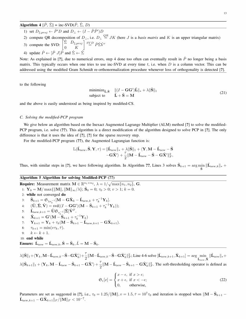
Algorithm 4 [P , Σ] = inc-SVD(P , Σ, D)

1) set D‖,proj ← P ′D and D⊥ ← (I − P P ′)D2) compute QR decomposition of D⊥, i.e. D⊥

QR= JK (here J is a basis matrix and K is an upper triangular matrix)

3) compute the SVD:[

Σ D‖,proj0 K

]SV D= P ΣV ′

4) update P ← [P J ]P and Σ← Σ

Note: As explained in [?], due to numerical errors, step 4 done too often can eventually result in P no longer being a basismatrix. This typically occurs when one tries to use inc-SVD at every time t, i.e. when D is a column vector. This can beaddressed using the modified Gram Schmidt re-orthonormalization procedure whenever loss of orthogonality is detected [?].

to the followingminimizeL,S ‖(I −GG′)L‖∗ + λ‖S‖1subject to L + S = M

(21)

and the above is easily understood as being inspired by modified-CS.

C. Solving the modified-PCP program

We give below an algorithm based on the Inexact Augmented Lagrange Multiplier (ALM) method [?] to solve the modified-PCP program, i.e. solve (??). This algorithm is a direct modification of the algorithm designed to solve PCP in [?]. The onlydifference is that it uses the idea of [?], [?] for the sparse recovery step.

For the modified-PCP program (??), the Augmented Lagrangian function is:

L(Lnew, S,Y, τ) = ‖Lnew‖∗ + λ‖S‖1 + 〈Y,M− Lnew − S

−GX′〉+τ

2‖M− Lnew − S−GX′‖2F ,

Thus, with similar steps in [?], we have following algorithm. In Algorithm ??, Lines 3 solves Sk+1 = arg minS‖Lnew,k‖∗ +

Algorithm 5 Algorithm for solving Modified-PCP (??)Require: Measurement matrix M ∈ Rn1×n2 , λ = 1/

√maxn1, n2, G.

1: Y0 = M/max‖M‖, ‖M‖∞/λ; S0 = 0; τ0 > 0; v > 1; k = 0.2: while not converged do3: Sk+1 = Sλτ−1

k[M−GXk − Lnew,k + τ−1

k Yk].4: (U, Σ, V) = svd((I −GG′)(M− Sk+1 + τ−1

k Yk));5: Lnew,k+1 = USτ−1

k[Σ]VT .

6: Xk+1 = G′(M− Sk+1 + τ−1k Yk)

7: Yk+1 = Yk + τk(M− Sk+1 − Lnew,k+1 −GXk+1).8: τk+1 = min(vτk, τ).9: k ← k + 1.

10: end whileEnsure: Lnew = Lnew,k, S = Sk, L = M− Sk.

λ‖S‖1+〈Yk,M−Lnew,k−S−GX′k〉+τ

2‖M−Lnew,k−S−GX′k‖2F ; Line 4-6 solve [Lnew,k+1, Xk+1] = arg min

Lnew,X‖Lnew‖∗+

λ‖Sk+1‖1 + 〈Yk,M− Lnew − Sk+1−GX′〉+ τ

2‖M− Lnew − Sk+1−GX′k‖2F . The soft-thresholding operator is defined as

Sε[x] =

x− ε, if x > ε;

x+ ε, if x < −ε;0, otherwise,

(22)

Parameters are set as suggested in [?], i.e., τ0 = 1.25/‖M‖, v = 1.5, τ = 107τ0 and iteration is stopped when ‖M− Sk+1 −Lnew,k+1 −GXk+1‖F /‖M‖F < 10−7.

14

V. PERFORMANCE GUARANTEES FOR REPROCS AND MODIFIED-PCP

A. Results for ReProCS

In recently published work [?], we obtained the following partial result for ReProCS. We call it a partial result because itslast assumption depends on intermediate algorithm estimates. In ongoing work that will be presented at ICASSP 2015 [?] andat ISIT 2015 [?], we now have a complete correctness result. We state this later in Theorem ??.

Theorem 5.1. Consider Algorithm ??. Let c := cmax and r := r0 + (J − 1)c. Pick a ζ that satisfies

ζ ≤ min

(10−4

r2,

1.5× 10−4

r2f,

1

r3γ2∗

)Assume that the initial subspace estimate is accurate enough, i.e. ‖(I − P0P

′0)P0‖ ≤ r0ζ. If the following conditions hold:

1) The algorithm parameters are set as ξ = ξ0(ζ), 7ξ ≤ ω ≤ Smin − 7ξ, K = K(ζ), α ≥ αadd(ζ) where these quantitiesare defined in Definition 4.1 of [?].

2) Lt satisfies Model ?? or Model ?? with

a) 0 ≤ cj,new ≤ cmax for all j (thus rj ≤ rmax := r0 + Jcmax),b) the at’s mutually independent over t,c) ‖at‖∞ ≤ γ∗ for all t (at’s bounded);,

3) Slow subspace change holds: (??) holds with d = Kα; (??) holds with g+ = 1.41 and (??) holds with v = 1.2; and cand γnew are small enough so that 14ξ0(ζ) ≤ Smin.

4) Denseness holds: equation (??) holds with κ+2s,∗ = 0.3 and κ+

2s,new = 0.15

5) The matrices Dj,new,k := (I − Pj−1P′j−1− Pj,new,kP

′j,new,k)Pj,new and Qj,new,k := (I −Pj,newPj,new

′)Pj,new,k satisfy

maxj

max1≤k≤K

κs(Dj,new,k) ≤ κ+s := 0.152

maxj

max1≤k≤K

κ2s(Qj,new,k) ≤ κ+2s := 0.15

then, with probability at least (1− n−10), at all times, t, all of the following hold:

1) at all times, t,Tt = Tt and

‖et‖2 = ‖Lt − Lt‖2 = ‖St − St‖2 ≤ 0.18√cγnew + 1.2

√ζ(√r + 0.06

√c).

2) the subspace error SE(t) := ‖(I − P(t)P′(t))P(t)‖2 satisfies

SE(t) ≤

(r0 + (j − 1)c)ζ + 0.4cζ + 0.6k−1

if t ∈ Ij,k, k = 1, 2 . . .K

(r0 + jc)ζ if t ∈ Ij,K+1

≤

10−2

√ζ + 0.6k−1

if t ∈ Ij,k, k = 1, 2 . . .K

10−2√ζ if t ∈ Ij,K+1

3) the error et = St − St = Lt − Lt satisfies the following at various times

‖et‖2 ≤

0.18√c0.72k−1γnew+

1.2(√r + 0.06

√c)(r0 + (j − 1)c)ζγ∗

if t ∈ Ij,k, k = 1, 2 . . .K

1.2(r0 + jc)ζ√rγ∗ if t ∈ Ij,K+1

≤

0.18√c0.72k−1γnew + 1.2(

√r + 0.06

√c)√ζ

if t ∈ Ij,k, k = 1, 2 . . .K

1.2√r√ζ if t ∈ Ij,K+1

The above result says the following. Consider Algorithm ??. Assume that the initial subspace error is small enough. If thealgorithm parameters are appropriately set, if slow subspace change holds, if the subspaces are dense, if the condition numberof Cov[at,new] is small enough, and if the currently unestimated part of the newly added subspace is dense enough (this isan assumption on the algorithm estimates), then, w.h.p., we will get exact support recovery at all times. Moreover, the sparse

15

recovery error will always be bounded by 0.18√cγnew plus a constant times

√ζ. Since ζ is very small, γnew < Smin, and c

is also small, the normalized reconstruction error for recovering St will be small at all times. In the second conclusion, webound the subspace estimation error, SE(t). When a subspace change occurs, this error is initially bounded by one. The aboveresult shows that, w.h.p., with each projection PCA step, this error decays exponentially and falls below 0.01

√ζ within K

projection PCA steps. The third conclusion shows that, with each projection PCA step, w.h.p., the sparse recovery error aswell as the error in recovering Lt also decay in a similar fashion.

The most important limitation of the above result is that it requires an assumption on Dnew,k and Qnew,k which dependon intermediate algorithm estimates, Pj,new,k. Moreover, it studies an algorithm that requires knowledge of model parameters.The first limitation was removed in our recent work [?] and both limitations were removed in our very recent work [?]. Webriefly summarize the result of [?] using the notation and model of this bookchapter (this is the notation and model of ourearlier published work [?] and has minor differences from the notation and model used in [?]). The key point is to replacecondition 5 (which is an assumption that depends on intermediate algorithm estimates, Pj,new,k) by an assumption on supportchange of St. The new assumption just says that the support should change at least every β frames and when it does, thechange should be by at least s/ρ (with ρ2β being small enough) and it should be such that the sets of changed indices aremutually disjoint for a period of α frames.

Theorem 5.2 (Complete Correctness Result for ReProCS [?]). Consider Algorithm ?? but with sparse recovery done onlysimple `1 minimization and support recovery done only by thresholding; and with ξ, ω, α and K set as given below.

1) Replace condition 1) of Theorem ?? by the following: set algorithm parameters as ξ =√rnewγnew + (

√r+√rnew)

√ζ;

ω = 7ξ; K =⌈

log(0.16rnewζ)log(0.83)

⌉; and α = C(log(6(K + 1)J) + 11 log(n)) for a constant C ≥ Cadd with Cadd :=

32 · 1002 max16,1.2(√ζ+√rnewγnew)4

(rnewζλ−)2

2) Assume conditions 2), 3), 4) of Theorem ?? hold.3) Replace condition 5) of Theorem ?? by the following assumption on support change: Let tk, with tk < tk+1, denote the

times at which Tt changes and let T [k] denote the distinct sets.

a) Assume that Tt = T [k] for all times t ∈ [tk, tk+1) with (tk+1 − tk) < β and |T [k]| ≤ s.b) Let ρ be a positive integer so that for any k,

T [k] ∩ T [k+ρ] = ∅;

assume thatρ2β ≤ 0.01α.

c) For any k,k+α∑i=k+1

∣∣∣T [i] \ T [i+1]∣∣∣ ≤ n

and for any k < i ≤ k + α,(T [k] \ T [k+1]) ∩ (T [i] \ T [i+1]) = ∅.

(One way to ensure∑k+αi=k+1 |T [i] \ T [i+1]| ≤ n is to require that for all i, |T [i] \ T [i+1]| ≤ s

ρ2with s

ρ2α ≤ n.)

Then all conclusions of Theorem ?? hold.

One example application that satisfies the above model on support change is a video application consisting of a foregroundwith one object of length s or less that can remain static for at most β frames at a time. When it moves, it moves downwards(or upwards, but always in one direction) by at least s/ρ pixels, and at most s/ρ2 pixels. Once it reaches the bottom of thescene, it disappears. The maximum motion is such that, if the object were to move at each frame, it still does not go from thetop to the bottom of the scene in a time interval of length α, i.e. s

ρ2α ≤ n. Anytime after it has disappeared another object

could appear.

B. Modified-PCP correctness result: static and online robust PCA cases

1) Modified-PCP correctness result for the static case: Consider the modified-PCP program given in (??). As explained in[?], we need that S is not low rank in order to separate it from Lnew in a batch fashion (recall that modified-PCP is a batchprogram; modified-PCP for online robust PCA is a piecewise batch solution). One way to ensure that S is full rank w.h.p. isby selecting the support of S uniformly at random [?]. We assume this here too. In addition, we need a denseness assumptionon the columns of G and on the left and right singular vectors of Lnew.

16

Let n(1) = max(n1, n2) and n(2) = min(n1, n2). Assume that following hold with a constant ρr

maxi‖[G Unew]′ei‖2 ≤

ρrn(2)

n1 log2 n(1)

, (23)

maxi‖V′newei‖2 ≤

ρrn(2)

n2 log2 n(1)

, (24)

and

‖UnewV′new‖∞ ≤√

ρr

n(1) log2 n(1)

. (25)

Theorem 5.3. Consider the problem of recovering L and S from M using partial subspace knowledge G by solving modified-PCP (??). Assume that Ω, the support set of S, is uniformly distributed with size m satisfying

m ≤ 0.4ρsn1n2 (26)

Assume that L satisfies (??), (??) and (??) and ρs, ρr, are small enough and n1, n2 are large enough. The explicit bounds areavailable in Assumption 3.2 of [?]. Then, Modified-PCP (??) with λ = 1/

√n(1) recovers S and L exactly with probability at

least 1− 23n−10(1) .

2) Modified-PCP correctness result for online robust PCA: Consider the online / recursive robust PCA problem where datavectors Mt := St + Lt come in sequentially and their subspace can change over time. Starting with an initial knowledge ofthe subspace, the goal is to estimate the subspace spanned by L1, L2, . . . Lt and to recover the St’s. For the above model, thefollowing is an easy corollary.

Corollary 5.4 (modified-PCP for online robust PCA). Assume Model ?? holds with∑j(cj,new − cj,old) ≤ cdif . Let Mj :=

[Mtj ,Mtj+1, . . .Mtj+1−1], Lj := [Ltj , Ltj+1, . . . Ltj+1−1], Sj := [Stj , Stj+1, . . . Stj+1−1] and let Lfull := [L1,L2, . . .LJ ] andSfull := [S1,S2, . . .SJ ]. Suppose that the following hold.

1) Sfull satisfies the assumptions of Theorem ??.2) The initial subspace span(P0) is exactly known, i.e. we are given P0 with span(P0) = span(P0).3) For all j = 1, 2, . . . J , (??), (??), and (??) hold with n1 = n, n2 = tj+1 − tj , G = Pj−1, Unew = Pj,new and Vnew

being the matrix of right singular vectors of Lnew = (I−Pj−1P′j−1)Lj .

4) We solve modified-PCP at every t = tj+1, using M = Mj and with G = Gj = Pj−1 where Pj−1 is the matrix of leftsingular vectors of the reduced SVD of Lj−1 (the low-rank matrix obtained from modified-PCP on Mj−1). At t = t1we use G = P0.

Then, modified-PCP recovers Sfull,Lfull exactly and in a piecewise batch fashion with probability at least (1− 23n−10)J .

Discussion w.r.t. PCP. Two possible corollaries for PCP can be stated depending on whether we want to compare PCP andmod-PCP when both have the same memory and time complexity or when both are provided the same total data.

The following is the corollary for PCP applied to the entire data matrix Mfull in one go. With doing this, PCP gets all thesame data that modified-PCP has access to. But PCP needs to store the entire data matrix in memory and also needs to operateon it, i.e. its memory complexity is roughly J times larger than that for modified-PCP and its time complexity is poly(J)

times larger than that of modified-PCP.

Corollary 5.5 (PCP for online robust PCA). Assume Model ?? holds with∑j(cj,new − cj,old) ≤ cdif . If Sfull satisfies the

assumptions of Theorem ?? and if (??), (??), and (??) hold with n1 = n, n2 = tJ+1 − t1, GPCP = [ ], Unew,PCP = U =

[P0,P1,new, . . .PJ,new] and Vnew,PCP = V being the right singular vectors of Lfull := [L1,L2, . . .LJ ], then, we can recoverLfull and Sfull exactly with probability at least (1− 23n−10) by solving PCP (??) with input Mfull. Here Mfull := Lfull + Sfull.

When we compare this with the result for modified-PCP, the second and third condition are clearly significantly weaker thanthose for PCP. The first conditions cannot be easily compared. The LHS contains at most rmax + c = r0 + cdif + c columnsfor modified-PCP, while it contains r0 +Jc columns for PCP. However, the RHS for PCP is also larger. If tj+1− tj = d, thenthe RHS is also J times larger for PCP than for modified-PCP. Thus with the above PCP corollary, the first condition of theabove and of modified-PCP cannot be compared.

The above advantages for mod-PCP come with two caveats. First, modified-PCP assumes knowledge of the subspace changetimes while PCP does not need this. Secondly, modified-PCP succeeds w.p. (1−23n−10)J ≥ 1−23Jn−10 while PCP succeedsw.p. 1− 23n−10.

17

Alternatively if PCP is solved at every t = tj+1 using Mj , we get the following corollary. This keeps the memory and timecomplexity of PCP the same as that for modified-PCP, but PCP gets access to less data than modified-PCP.

Corollary 5.6 (PCP for Mj). Assume Model ?? holds with∑j(cj,new− cj,old) ≤ cdif . Solve PCP, i.e. (??), at t = tj+1 using

Mj . If Sfull satisfies the assumptions of Theorem ?? and if (??), (??), and (??) hold with n1 = n, n2 = tj+1− tj , GPCP = [ ],Unew,PCP = Pj and Vnew,PCP = Vj being the right singular vectors of Lj for all j = 1, 2, . . . , J , then, we can recoverLfull and Sfull exactly with probability at least (1− 23n−10)J .

When we compare this with modified-PCP, the second and third condition are significantly weaker than those for PCP whencj,new rj . The first condition is exactly the same when cj,old = 0 and is only slightly stronger as long as cj,old rj .

C. Discussion

In this discussion we use the correctness result of Theorem ?? for ReProCS. This was proved in our very recent work [?].We should point out first that the matrix completion problem can be interpreted as a special case of the robust PCA problemwhere the support sets Tt are the set of missing entries and hence are known. Thus an easy corollary of our result is a resultfor online matrix completion. This can be compared with the corresponding result for nuclear norm minimization (NNM) [?]from [?].

Our result requires accurate initial subspace knowledge. As explained earlier, for video analytics, this corresponds to requiringan initial short sequence of background-only video frames whose subspace can be estimated via SVD (followed by using asingular value threshold to retain a certain number of top left singular vectors). Alternatively if an initial short sequence of thevideo data satisfies the assumptions required by a batch method such as PCP, that can be used to estimate the low-rank part,followed by SVD to get the column subspace.

In Model ?? or ?? and the slow subspace change assumption, we are placing a slow increase assumption on the eigenvaluesalong the new directions, Ptj ,new, only for the interval [tj , tj+1). Thus after tj+1, the eigenvalues along Ptj ,new can increasegradually or suddenly to any large value up to λ+.

The assumption on Tt is a practical model for moving foreground objects in video. We should point out that this model isone special case of the general set of conditions that we need (see Model 5.1 of [?]).

As explained in [?], the model on Tt and the denseness condition of the theorem constrain s and s, r0, rnew, J respectively.The model on Tt requires s ≤ ρ2n/α for a constant ρ2. Using the expression for α, it is easy to see that as long as J ∈ O(n),we have α ∈ O(log n) and so this needs s ∈ O( n

logn ). With s ∈ O( nlogn ), using (??), it is easy to see that the denseness

condition will hold if r0 ∈ O(log n), J ∈ O(log n) and rnew is a constant. This is one set of sufficient conditions that weallow on the rank-sparsity product.

Let Lfull := [L1, L2, . . . , Ltmax ] and Sfull := [S1, S2, . . . , Stmax ]. Let rmat := rank(Lfull). Clearly rmat ≤ r0 + Jrnew andthe bound is tight. Let smat := tmaxs be a bound on the support size of the outliers’ matrix Sfull. In terms of rmat and smat,what we need is rmat ∈ O(log n) and smat ∈ O(ntmax

logn ). This is stronger than what the PCP result from [?] needs ([?] allows

rmat ∈ O(

n(logn)2

)while allowing smat ∈ O(ntmax)), but is similar to what the PCP results from [?], [?] need.

Other disadvantages of our result are as follows. (1) Our result needs accurate initial subspace knowledge and slow subspacechange of Lt. As explained earlier and in [?, Fig. 6], both of these are often practically valid for video analytics applications.Moreover, we also need the Lt’s to be zero mean and mutually independent over time. Zero mean is achieved by letting Ltbe the background image at time t with an empirical ‘mean background image’, computed using the training data, subtractedout. The independence assumption then models independent background variations around a common mean. As we explain inSection ??, this can be easily relaxed and we can get a result very similar to the current one under a first order autoregressivemodel on the Lt’s. (2) Moreover, ReProCS needs four algorithm parameters to be appropriately set. The PCP or NNM resultsneed this for none [?], [?] or at most one [?], [?] algorithm parameter. (3) Thirdly, our result for online RPCA also needs alower bound on Smin while the PCP results do not need this. (4) Moreover, even with this, we can only guarantee accuraterecovery of Lt, while PCP or NNM guarantee exact recovery.

(1) The advantage of our work is that we analyze an online algorithm (ReProCS) that is faster and needs less storagecompared with PCP or NNM. It needs to store only a few n×α or n×rmat matrices, thus the storage complexity is O(n log n)

while that for PCP or NNM is O(ntmax). In general tmax can be much larger than log n. (2) Moreover, we do not need anyassumption on the right singular vectors of L while all results for PCP or NNM do. (3) Most importantly, our results allowhighly correlated changes of the set of missing entries (or outliers). From the assumption on Tt, it is easy to see that weallow the number of missing entries (or outliers) per row of L to be O(tmax) as long as the sets follow the support change

18

assumption 4. The PCP results from [?], [?] need this number to be O( tmax

rmat) which is stronger. The PCP result from [?] or

the NNM result [?] need an even stronger condition - they need the set (∪tmaxt=1 Tt) to be generated uniformly at random.

In [?], Feng et. al. propose a method for online RPCA and prove a partial result for their algorithm. The approach is toreformulate the PCP program and use this reformulation to develop a recursive algorithm that converges asymptotically tothe solution of PCP as long as the basis estimate Pt is full rank at each time t. Since this result assumes something aboutthe algorithm estimates, it is also only a partial result. Another somewhat related work is that of Feng et. al. [?] on onlinePCA with contaminated data. This does not model the outlier as a sparse vector but defines anything that is far from the datasubspace as an outlier.

To compare with the correctness result of modified-PCP given earlier, two things can be said. First, like PCP, the resultfor modified PCP also needs uniformly randomly generated support sets. But its advantage is that its assumption on therank-sparsity product is weaker than that of PCP, and hence weaker than that needed by ReProCS. Also see the simulations’section.

VI. NUMERICAL EXPERIMENTS

A. Simulation experiments

1) Comparing ReProCS and PCP: We first provide some simulations that demonstrate the result we have proven above forReProCS and how it compares with the result for PCP.

The data for Figure ?? was generated as follows. We chose n = 256 and tmax = 15, 000. Each measurement had s = 20

missing or corrupted entries, i.e. |Tt| = 20. Each non-zero entry of the sparse vector was drawn uniformly at random between2 and 6 independent of other entries and other times t. In Fig. ?? the support of St changes as assumed Theorem ?? withρ = 2 and β = 18. So Tt changes by s

2 = 10 indices every 18 time instants. When it reaches the bottom of the vector, it startsover again at the top. This pattern can be seen in the bottom half of the figure which shows the sparsity pattern of the matrixS

To form the low dimensional vectors Lt, we started with an n× r matrix of i.i.d. Gaussian entries and orthonormalized thecolumns using Gram-Schmidt. The first r0 = 10 columns of this matrix formed P(0), the next 2 columns formed P(1),new, andthe last 2 columns formed P(2),new We show two subspace changes which occur at t1 = 600 and t2 = 8000. The entries ofat,∗ were drawn uniformly at random between -5 and 5, and the entries of at,new were drawn uniformly at random between

−√

3vt−tji λ− and

√3vt−tji λ− with vi = 1.00017 and λ− = 1. Entries of at were independent of each other and of the other

at’s.For this simulated data we compare the performance of ReProCS and PCP. The plots show the relative error in recovering

Lt, that is ‖Lt − Lt‖2/‖Lt‖2. For the initial subspace estimate P0, we used P0 plus some small Gaussian noise and thenobtained orthonormal columns. We set α = 800 and K = 6. For the PCP algorithm, we perform the optimization every α

time instants using all of the data up to that point. So the first time PCP is performed on [M1, . . . ,Mα] and the second timeit is performed on [M1, . . . ,M2α] and so on.

Figure ?? illustrates the result we have proven in Theorem ??. That is ReProCS takes advantage of the initial subspaceestimate and slow subspace change (including the bound on γnew) to handle the case when the supports of St are correlatedin time. Notice how the ReProCS error increases after a subspace change, but decays exponentially with each projection PCAstep. For this data, the PCP program fails to give a meaningful estimate for all but a few times. The average time taken by theReProCS algorithm was 52 seconds, while PCP averaged over 5 minutes. Simulations were coded in MATLABr and run on adesktop computer with a 3.2 GHz processor. Compare this to Figure ?? where the only change in the data is that the supportof S is chosen uniformly at random from all sets of size stmax

n (as assumed in [?]). Thus the total sparsity of the matrix S isthe same for both figures. In Figure ??, ReProCS performs almost the same as in Fig. ??, while PCP does substantially betterthan in the case of correlated supports.

2) Comparing Modified-PCP, ReProCS, PCP and other algorithms: We generated data using Model ?? with n = 256,J = 3, r0 = 40, t0 = 200 and cj,new = 4, cj,old = 4, for each j = 1, 2, 3. We used t1 = t0 + 6α+ 1, t2 = t0 + 12α+ 1 andt3 = t0 + 18α+ 1 with α = 100, tmax = 2600 and γ = 5. The coefficients, at,∗ = P′j−1Lt were i.i.d. uniformly distributed inthe interval [−γ, γ]; the coefficients along the new directions, at,new := P′j,newLt generated i.i.d. uniformly distributed in theinterval [−γnew, γnew] (with a γnew ≤ γ) for the first 1700 columns after the subspace change and i.i.d. uniformly distributed inthe interval [−γ, γ] after that. We vary the value of γnew; small values mean that “slow subspace change” required by ReProCS

4In a period of length α, the set Tt can occupy index i for at most ρβ time instants, and this pattern is allowed to repeat every α time instants. So anindex can be in the support for a total of ρβ tmax

αtime instants and the model assumes ρβ ≤ 0.01α

ρfor a constant ρ.

19

(a) correlated support change (b) uniformly randomly selected support sets

Fig. 3. Comparison of ReProCS and PCP for the RPCA problem. In each subfigure, the top plot is the relative error ‖Lt − Lt‖2/‖Lt‖2. The bottom plotshows the sparsity pattern of S (black represents a non-zero entry). Results are averaged over 100 simulations and plotted every 300 time instants.

holds. The sparse matrix S was generated in two different ways to simulate uncorrelated and correlated support change. Forpartial knowledge, G, we first did SVD decomposition on [L1, L2, · · · , Lt0 ] and kept the directions corresponding to singularvalues larger than E(z2)/9, where z ∼ Unif[−γnew, γnew]. We solved PCP and modified-PCP every 200 frames by using theobservations for the last 200 frames as the matrix M. The ReProCS algorithm was implemented with α = 100. The averagedsparse part errors with two different sets of parameters over 20 Monte Carlo simulations are displayed in Fig. ?? and Fig. ??.

In the first case, Fig. ??, we used γnew = γ and so “slow subspace change” does not hold. For the sparse vectors St, eachindex is chosen to be in support with probability 0.0781. The nonzero entries are uniformly distributed between [20, 60]. Since“slow subspace change” does not hold, ReProCS does not work well. Since the support is generated independently over time,this is a good case for both PCP and mod-PCP. Mod-PCP has the smallest sparse recovery error. In the second case, Fig. ??,we used γnew = 1 and thus “slow subspace change” holds. For sparse vectors, St, the support is generated in a correlatedfashion. We used support size s = 10 for each St; the support remained constant for 25 columns and then moved down bys/2 = 5 indices. Once it reached n, it rolled back over to index one. Because of the correlated support change, PCP does notwork. In this case, the sparse vectors are highly correlated over time, resulting in sparse matrix S that is even more low rank,thus neither mod-PCP nor PCP work for this data. In this case, only ReProCS works.

Thus from simulations, modified-PCP is able to handle correlated support change better than PCP but worse than ReProCS.Modified-PCP also works when slow subspace change does not hold; this is a situation where ReProCS fails. Of course,modified-PCP, GRASTA and ReProCS are provided the same partial subspace knowledge G.

B. Video experiments

We show comparisons on two real video sequences. These are originally taken from http://perception.i2r.a-star.edu.sg/bkmodel/bk index.html and http://research.microsoft.com/en-us/um/people/jckrumm/wallflower/testimages.htm, respectively. Thefirst is an indoor video of window curtains moving due to the wind. There was also some lighting variation. The latter part ofthis sequence also contains a foreground (various persons coming in, writing on the board and leaving). For t > 1755, in theforeground, a person with a black shirt walks in, writes on the board and then walk out, then a second person with a white shirtdoes the same and then a third person with a white shirt does the same. This video is challenging because (i) the white shirtcolor and the curtains’ color is quite similar, making the corresponding St small in magnitude; and (ii) because the backgroundvariations are quite large while the foreground person moves slowly. As can be seen from Fig. ??, ReProCS’s performance issignificantly better than that of the other algorithms for both foreground and background recovery. This is most easily seenfrom the recovered background images. One or more frames of the background recovered by PCP, RSL and GRASTA containsthe person, while none of the ReProCS ones does.

The second sequence consists of a person entering a room containing a computer monitor that contains a white movingregion. Background changes due to lighting variations and due to the computer monitor. The person moving in the foregroundoccupies a very large part of the image, so this is an example of a sequence in which the use of weighted `1 is essential (the

20

500 1000 1500 2000 250010

−8

10−6

10−4

10−2

100

102

t

‖s t

−s t‖/‖s t‖

ReProCSPCPmod−PCPGRASTARSLGOSUS

(a) uniformly distributed Tt’s, slow subspace change does not hold

0 2000 4000 6000 8000

10−15

10−10

10−5

100

t

‖s t

−s t‖/‖s t‖

ReProCSPCPmod−PCPGRASTARSLGOSUS

(b) correlated Tt’s, slow subspace change holds

Fig. 4. NRMSE of sparse part (n = 256, J = 3, r0 = 40, t0 = 200, cj,new = 4, cj,old = 4, j = 1, 2, 3)

original ReProCS PCP RSL GRASTA MG ReProCS PCP RSL GRASTA MG(fg) (fg) (fg) (fg) (fg) (bg) (bg) (bg) (bg) (bg)

Fig. 5. Original video sequence at t = ttrain + 60, 120, 199, 475, 1148 and its foreground (fg) and background (bg) layer recovery resultsusing ReProCS (ReProCS-pCA) and other algorithms. For fg, we only show the fg support in white for ease of display.

support size is too large for simple `1 to work). As can be seen from Fig. ??, for most frames, ReProCS is able to recoverthe person correctly. However, for the last few frames which consist of the person in a white shirt in front of the white partof the screen, the resulting St is too small even for ReProCS to correctly recover. The same is true for the other algorithms.Videos of all above experiments and of a few others are posted at http://www.ece.iastate.edu/∼hanguo/PracReProCS.html.

Time Comparisons. The time comparisons are shown in Table ??. In terms of speed, GRASTA is the fastest even thoughits performance is much worse. ReProCS is the second fastest. We expect that ReProCS can be speeded up by using mex files(C/C++ code) for the subspace update step. PCP and RSL are slower because they jointly process the entire image sequence.Moreover, ReProCS and GRASTA have the advantage of being recursive methods, i.e. the foreground/background recovery isavailable as soon as a new frame appears while PCP or RSL need to wait for the entire image sequence.

VII. CONCLUSIONS AND FUTURE WORK

In this bookchapter we provided an overview of our recent work on the online or recursive robust PCA problem. Weexplained both the key idea of the ReProCS algorithm proposed in our recent work to solve this problem and how to developits practical modification that can be directly used with real datasets. Extensive numerical experiments - both with simulateddata and real videos - were shown demonstrating the advantage of ReProCS over many existing algorithms for robust PCA

21

original ReProCS PCP RSL GRASTA MG ReProCS PCP RSL GRASTA MG(fg) (fg) (fg) (fg) (fg) (bg) (bg) (bg) (bg) (bg)

Fig. 6. Original video sequence at t = ttrain + 42, 44, 52 and its foreground (fg) and background (bg) layer recovery results using ReProCS(ReProCS-pCA) and other algorithms. For fg, we only show the fg support in white for ease of display.

DataSet Image Size Sequence Length ReProCS-pPCA ReProCS-Recursive-PCA PCP RSL GRASTALake 72× 90 1420 + 80 2.99 + 19.97 sec 2.99 + 19.43 sec 245.03 sec 213.36 sec 39.47 + 0.42 sec

Curtain 64× 80 1755 + 1209 4.37 + 159.02 sec 4.37 + 157.21 sec 1079.59 sec 643.98 sec 40.01 + 5.13 secPerson 120× 160 200 + 52 0.46 + 42.43 sec 0.46 + 41.91 sec 27.72 sec 121.31 sec 13.80 + 0.64 sec

TABLE ICOMPARISON OF SPEED OF DIFFERENT ALGORITHMS. EXPERIMENTS WERE DONE ON A 64 BIT WINDOWS 8 LAPTOP WITH 2.40GHZ I7CPU AND 8G RAM. SEQUENCE LENGTH REFERS TO THE LENGTH OF SEQUENCE FOR TRAINING PLUS THE LENGTH OF SEQUENCE FOR

SEPARATION. FOR REPROCS AND GRASTA, THE TIME IS SHOWN AS TRAINING TIME + RECOVERY TIME.

- both batch and recursive. We also summarized and discussed the performance guarantees for ReProCS in detail. Lastly webriefly described our work on modified-PCP which is a piecewise batch approach that removes a key limitation of ReProCS(it allows a looser bound on the rank-sparsity product as compared with ReProCS), however it retains a key limitation of PCP(like PCP it also cannot handle highly correlated support change as well as ReProCS). Its correctness result was also givenand discussed.

The tools introduced to prove the correctness result for ReProCS in [?], [?], [?] can also be used to get a correctness resultfor a practical modification of ReProCS with cluster-PCA (ReProCS-cPCA) which is Algorithm 2 of [?]. This algorithm wasintroduced to also remove the deleted directions from the subspace estimate. It does this by re-estimating the previous subspaceat a time after the newly added subspace has been accurately estimated (i.e. at a time after tj + Kα). A partial result forthis algorithm was proved in [?]. This result will need one extra assumption – it will need the eigenvalues of the covariancematrix of Lt to be clustered for a period of time after the subspace change has stabilized, i.e. for a period of d2 frames inthe interval [tj + d + 1, tj+1 − 1] – but it will have a key advantage. It will need a much weaker denseness assumption andhence a much weaker bound on r or rmat. In particular, with this result we expect to be able to allow r = rmat ∈ O(n) withthe same assumptions on s and smat that we currently allow. This requirement is almost as weak as that of PCP.

The results for ReProCS presented here assume that the Lt’s are independent over time and zero mean; this is a valid modelwhen background images have independent random variations about a fixed mean. Using the tools developed in these works,a similar result can also be obtained for the more general case of Lt’s following an autoregressive model. This will allow theLt’s to be correlated over time. A partial result for this case was obtained in [?]. The main change in this case will be thatwe will need to apply the matrix Azuma inequality from [?] instead of matrix Hoeffding. This is will also require algebraicmanipulation of sums and some other important modifications, as explained in [?], so that the constant term after conditioningon past values of the matrix is small.

We expect that the tools introduced in [?], [?], [?] can also be used to analyze the noisy case, i.e. the case of Mt = St+Lt+wt

where wt is small bounded noise. In most practical video applications, while the foreground is truly sparse, the backgroundis only approximately low-rank. The modeling error can be treated as as wt. The proposed algorithms already apply withoutmodification to this case (see [?] for results on real videos).

Finally, we expect both the algorithm and the proof techniques to apply with simple changes to the undersampled caseMt = AtSt + BtLt + wt as long as Bt is not time-varying, i.e. Bt = B0. A partial result for this case was obtained in [?]and experiments were shown in [?].

In other ongoing work, we are working to replace the ell-1 minimization in the projected sparse recovery step by algorithmsdesigned under various other structured sparsity assumptions that may be valid for a given problem. For example, in [?], weintroduced the support predicted modified-CS algorithm that uses a motion model to predict a moving object’s support in the

22

next frame and uses the predicted support as partial subspace knowledge for modified-CS. The motion model parameters arethemselves tracked using a Kalman filter.