1

Notes on Boltzmann MachinesPatrick Kenny

Centre de recherche informatique de MontrealPatrick.Kenny@crim.ca

I. INTRODUCTION

Boltzmann machines are probability distributions on high dimensional binary vectors which are analogous to GaussianMarkov Random Fields in that they are fully determined by first and second order moments. A key difference howeveris that augmenting Boltzmann machines with hidden variables enlarges the class of distributions that can be modeled, sothat in principle it is possible to model distributions of arbitrary complexity [1]. (On the other hand, marginalizing overhidden variables in a Gaussian distribution merely gives another Gaussian.) Training Boltzmann machines still seems to bemore of an art than a science, but a variational Bayes expectation maximization algorithm has been developed which dealswith this problem in a reasonably efficient way for a class of sparsely connected Boltzmann machines that includes the deepBoltzmann machines studied in [2]. I will explain how this approach provides a principled framework for constructing complexBoltzmann machines incrementally and how it can be extended straightforwardly to handle higher order Boltzmann machines(e.g. Boltzmann machines defined by third order moments).

The binary/Gaussian distinction is not an exclusive dichotomy: hybrid models containing both types of variable can beconstructed. The term Gaussian-Bernoulli Boltzmann machine is usually used to refer to a model in which the vector of visiblevariables v is continuous and the vector of hidden variables h is binary. For each binary configuration h, the conditionaldistribution of v given h is Gaussian so writing

P (v) =∑h

P (h)P (v|h)

shows that this model can be interpreted as a Gaussian mixture with a prodigious number of components.1 This type of modelis frequently use to binarize continuous data (for example it would be possible in to associate with each data vector v, themaximum a posteriori estimate of h) so that binary Boltzmann machines can be used in subsequent processing. In speechprocessing applications, a model like this can be used as a Universal Background Model and it can accommodate data vectorsof much higher dimension than traditional Gaussian mixture models. In particular, cepstral coefficients extracted from 10 – 15frames can be concatenated and treated as a single data vector.

Boltzmann machines may be used to implement either generative or discriminative approaches to pattern recognitionproblems. Broadly speaking, generative approaches work best in speaker recognition and discriminative approaches workbest in speech recogntion. State of the art speaker recognition systems use several types of generative model as featureextractors (the Universal Background Model, Joint Factor Analysis and the i-vector extractor) and as classifiers (ProbabilisticLinear Discriminant Analysis and the cosine distance metric) [4], [5], [6]. These generative models rely heavily on Gaussianassumptions, some of which are quite questionable. Using Boltzmann machines to develop alternative generative models forspeaker recognition promises to be an interesting line of research. I will sketch very briefly how such a program might becarried out.

In the machine learning literature, Boltzmann machines are principally used in unsupervised training of another type ofgenerative model known as a sigmoid belief network or deep belief network (DBN). The hidden variables in a DBN can bethought of as providing causal explanations of data so that calculating the posteriors of the hidden variables in the DBN canbe viewed as a sort of high level feature extraction. The standard (mean-field) approximation used for posterior calculationsin a DBN is implemented by a feed forward neural net (where the top level softmax layer usually used to make recognitiondecisions is missing). Suppose then that a DBN can be trained in an unsupervised way on a given data population in such away that the high level feature extractors learned in the course of training are useful for recognizing patterns in the data. Undersuch circumstances, it would be reasonable to use the posterior calculations in the DBN as an initialization for backpropagationtraining of a feed forward neural network designed to discriminate between these patterns.

This strategy has been successfully deployed in speech recognition, notably at Microsoft. Interestingly, Microsoft has alsorecently reported excellent speech recognition results obtained with unaided backpropagation in deep neural nets [7] (that is,without using a DBN-based initialization) so the question of whether deep belief networks will play an important role in speechrecognition in the future remains to be settled.

For background reading, the principal reference is [1]. See also [8], [3] (particularly the Chapter on Boltzmann machines)and [9] (Chapter 11). The January 2012 issue of the IEEE Transactions on Audio, Speech and Language Processing containeda special section on Deep Learning.

1To get an idea of how large the number 21000 is, see Chapter 29 of [3].

2

II. PRELIMINARIES

This section summarizes the probabilistic arguments needed to understand the literature on Boltzmann machines and deepbelief networks. See [8].

Conventions We use P (·) to indicate probabilities calculated with a given model, irrespective of whether these probabilitiescan be evaluated exactly or not. As a rule, we use the symbol Q(·) to refer to posterior probabilities of hidden variables givendata. These posteriors may be approximate or exact, depending on the context.

We use h to denote hidden vector-valued variables, v to denote visible variables and x to denote generic variables (insituations where there is no need to distinguish between hidden and visible variables).

The Kullback-Leibler divergence between two distributions P1(x) and P2(x) is denoted by D (P1(x) || P2(x)) and given by

D (P1(x) || P2(x)) =∑x

P1(x) lnP1(x)P2(x)

.

It has the property that D (P1(x) || P2(x)) ≥ 0 with equality iff P1 and P2 are identical. The divergence is an asymmetricmeasure of the difference between the two distributions.

The entropy of P (x) is denoted by H(P (x)) and given by

H(P (x)) = −∑x

P (x) lnP (x).

It has the property that H(P (x)) ≥ 0 with equality iff P (x) is concentrated on a single value of x.

A. The evidence inequality

Suppose we have a model with both hidden and visible variables. The marginal probability of the visible variables, givenby

P (v) =∑h

P (v,h)

is known as the evidence. For interesting models, this summation is intractable. The problem of evaluating or approximatingP (v) turns out to be equivalent to the problem of evaluating or approximating the posterior Q(h|v).

Define

L = E

[lnP (v,h)Q(h|v)

]where the expectation is taken with respect to Q(h|v) which may be the exact posterior or an approximate posterior.

This can be written in several different forms, all of them useful:

E [lnP (v,h)] +H(Q(h|v))E [lnP (v|h)]− D (Q(h|v) || P (h))

lnP (v)− D (Q(h|v) || P (h|v)) .

The first follows from the definition of L and the second from the first (write P (v,h) = P (v|h)P (h)). In the third expression,we use the notation P (h|v) to indicate the exact posterior of h given v so that

L = E

[lnP (v,h)Q(h|v)

]= E

[lnP (h|v)P (v)Q(h|v)

]= lnP (v) + E

[lnP (h|v)Q(h|v)

]= lnP (v)− D (Q(h|v) || P (h|v)) .

The non-negativity property of the Kullback-Leibler divergence implies that L ≤ lnP (v) with equality holding iff the posterioris exact. This is the evidence inequality.

The lower bound is sometimes written as

〈lnP (v,h)〉data +H

where “data” refers to the posterior distribution Q(h|v). (Similarly, 〈·〉model is used to refer to an expectation taken withrespect to the prior distribution P (v,h).)

The quantity E [lnP (v,h)] is known as the EM auxiliary function.

3

B. The EM algorithm

If we are given a training set consisting of a collection of visible vectors {vn}, the lower bound is given by

L =∑

n

EQ(h|vn)

[lnP (h,vn)Q(h|vn)

].

Evaluating these expectations is the E-step of the EM algorithm.In order to fit the model to the data we want to make L as large as possible. L can be increased in two ways:1) Fix the posteriors Q(h|vn) and adjust the parameters of the model P (v,h) so as to increase the EM auxiliary function∑

n

∑h

Q(h|vn) lnP (h,vn)

2) Fix the model P (v,h) and adust the posteriors Q(h|vn) so as to decrease the divergence∑n

D (Q(h|vn) || P (h|vn)) .

WritinglnP (v,h) = lnP (h) + lnP (v|h),

we have 2 special cases of 1), namely adjusting P (v|h) so as to maximize∑

n

∑hQ(h|vn) lnP (vn|h) and adjusting P (h)

so as to maximize∑

n

∑hQ(h|vn) lnP (h). The latter is equivalent to minimizing the divergence∑

n

D (Q(h|vn) || P (h))

and is sometimes referred to as minimum divergence estimation of P (h).In the case where Q(h|v) = P (h|v) the lower bound is tight (lnP (v) = L) so alternating between 1) and 2) is guaranteed

to increase the likelihood of the training set. This is the classical EM algorithm.In the general case where an approximate variational posterior is used, the value of the lower bound is guaranteed to increase

but this does not guarantee that the likelihood increases. This is the variational Bayes EM algorithm

C. Variational Bayes

In situations where the posterior is intractable we can seek an approximation of the form

Q(h|v) =∏

i

Q(hi|v)

where the factors on the right hand side are chose so as to maximize L. Fix i and suppose we want to estimate Q(hi|v),assuming that Q(hjv) fixed for j 6= i. Writing h = (hi,h\i),

L = EQ(h|v)

[lnP (v,h)Q(h|v)

]= EQ(hi)

[EQ(h\i)

[lnP (hi,h\i,v)Q(hi)Q(h\i)

]]= EQ(hi)

[EQ(h\i)

[lnP (hi,h\i,v)

Q(hi)

]]+ constant

= EQ(hi)

[lnQ(hi)Q(hi)

]+ constant

= −D(Q(hi) || Q(hi)

)where Q(hi) is the distribution defined by

ln Q(hi) = EQ(h\i)

[lnP (hi,h\i,v)

]+ constant,

the constant being determined by the condition that∑

hiQ(hi) = 1. (In future, we will use the symbol ≡ to indicate equality

up to an irrelevant additive constant.) Thus to maximize L, we minimize the divergence and take Q(hi) = Q(hi). It is necessaryto cycle through the factors until convergence. (Convergence is guaranteed.)

4

D. Gibbs sampling

It may be the case that it is hard to sample from the prior P (x) but is easy to sample efficiently from the posterior distributionQ(xi|x\i). For example suppose x has just 2 components. We generate a Markov chain

x1 → x2 → . . .→ xn . . .

by taking a random value x02 and sampling

x11 ∼ Q(x1

1|x02), x

12 ∼ Q(x1

2|x11), x

21 ∼ Q(x2

1|x12), x

22 ∼ Q(x2

2|x21), . . . .

(Two samples are needed for each full step x1 → x2,x2 → x3, . . ..) For n sufficiently large, xn will be distributed accordingto P (x). (The model distribution is the equilibrium distribution of the Markov chain.)

The principle extends straightforwardly to posterior distributions so that samples can be drawn from a posterior Q(h|v) pro-vided that for each i it is easy to sample from Q(hi|h\i,v). Generally speaking Gibbs sampling is much more computationallyexpensive than variational Bayes (it is an exact method but variational Bayes is not).

III. BOLTZMANN MACHINES

A Boltzmann machine is a probability distribution on binary vectors x of the form

P (x) =1Ze−E(x)

where the “energy function” E(x) has the form

E(x) = −∑i<j

xiwijxj ,

the sum extending over all pairs (i, j) such that i < j. The normalizing constant Z is referred to as the partition function.Alternatively

E(x) = −12

∑i,j

xiwijxj ,

the sum extending over all pairs (i, j). Units are sometimes referred to as neurons and the weights wij as synaptic weights. Wedenote the weight matrix by W . Some of the units may be distinguished as visible and others as hidden. When it is necessaryto make this distinction we will use the symbol vi for the binary variable associated with a visible unit i and the symbol hj

for the binary variable associated with a hidden unit j. The matrix W is assumed to be symmetric with zero diagonal. (Thediagonal entries are forced to be zero to prevent neurons from interacting with themselves.) First order terms such as

∑j wjxj

could also be included but there is no gain in generality as this is equivalent to forcing some of the components of x to be 1.We will exclude these “bias” terms in order to keep the derivations simple.

Energy based models differ from probability distributions defined by directed acyclic graphs (Bayesian networks). Inparticular, it is not usually straightforward to evaluate the partition function and we will not address this question for Boltzmannmachines as it is not needed for the applications we have in mind (see [2], [8]). The energy function can be thought of asspecifying soft constraints on the data (regions of low energy – sometimes referred to as ravines in the energy surface – havehigh probability) and additional constraints can be imposed by adding terms to the energy function. But the energy functiondoes not provide a simple recipe for sampling from the probability distribution. (Some type of Markov Chain Monte Carlo(MCMC) method such as Gibbs sampling or the Metropolis algorithm is needed.)

A. Gibbs sampling

The Gibbs sampling formulas shows that a Boltzmann machine can be regarded as a stochastic neural network.

Q(xi = 1|x\i) =P (xi = 1,x\i)

P (xi = 0,x\i) + P (xi = 1,x\i)

=exp

(∑j 6=i wijxj

)1 + exp

(∑j 6=i wijxj

)= σ

∑j 6=i

wijxj

where σ is the sigmoid (that is, S-shaped) non-linearity defined by

σ(u) = (1 + e−u)−1.

5

It is easily verified that

σ(−u) + σ(u) = 1σ′(u) = σ(u)(1− σ(u)).

The argument of σ (rather than the value it returns), namely∑

j 6=i wijxj , is referred to in [8] as the activation of the unit iand σ is called the activation function.

B. The mean field approximation

In order to convert the Boltzmann machine into a deterministic neural network we can apply variational Bayes to the priordistribution P (x), that is, we calculate a variational approximation

P (x) ≈∏

i

Q(xi)

=∏

i

µxii

where µi = Q(xi = 1). (In the context of Boltzmann machines, variational Bayes is usually referred to as the mean fieldapproximation.)

The variational update equations are

lnQ(xi) ≡ EQ(x\i)

[lnP (xi,x\i)

]= EQ(x\i)

∑j 6=i

xiwijxj

=

{ ∑j 6=i wijµj if xi = 1

0 if xi = 0so

Q(xi = 1) =exp

(∑j 6=i wijµj

)1 + exp

(∑j 6=i wijµj

)= σ

∑j 6=i

wijµj

Since µi = Q(xi = 1), the fixed point equations are

µi = σ

∑j 6=i

wijµj

.

These are the same as the equations for Gibbs sampling except that the x’s are replaced by their mean values, the µ’s. Thisexplains the term “mean field” and shows how the Boltzmann distribution can be approximated by a deterministic neural net.

Note that the mean field approximation is not a good approximation to P (x) since it treats the units as statistically independentand the approximate distribution is unimodal. (A unimodal approximation is generally only reasonable for approximating theposterior of hidden variables given an observation. The hidden variables are usually thought of as explaining the observation;to say that the posterior distribution on the hidden variables is unimodal just means that there is only one way of explainingthe obseration.) In practice, variational Bayes should only be applied to posterior distributions, not prior distributions.

C. The Markov property

The most interesting situation is when the matrix W is sparse. Let x\{i,j} denote the set of variables other than xi and xj .If x\{i,j} is given and wij = 0 can write the energy function as

E(x) = axi + bxj + c

where a, b and c depend on x\{i,j} but not on xi or xj . Thus xi and xj are conditionally independent if x\{i,j} is given,provided that wij = 0.

A Boltzmann machine is represented by a graphical model with undirected edges joining all pairs of vertices i, j for whichwij is not zero. The conditional independence property can be generalized as follows. Suppose we are given a partition of theunits into three subsets A, B and C with the property that there is no edge between vertices in A and C. Then xA and xC

6

are conditionally independent if xB is given where xA = {xi : i ∈ A} etc. This is called the Markov property: the “future”(C) is independent of the “past” (A) if the “present” (B) is given.

So the graph provides information about how conditional distributions such as P (·|xB) factorize. (This is different fromthe case of directed graphical models where the topology of the graph tells you how the prior distribution factorizes.) Withpractice, it is possible to tell by inspecting an undirected graphichal model whether Gibbs sampling and variational Bayes arepractically feasible.

Restricted Boltzmann machines In this case there is a hidden layer and a visible layer with no hidden-to-hidden or visible-to-visible connections. The vectors h,v are of dimension J × 1 and I × 1 and W is of dimension I × J . The energy functionis

E(v,h) = −vTWh.

By the Markov property, Q(h|v) and P (v|h) both factorize

Q(h|v) =∏j

Q(hj |v)

P (v|h) =∏

i

P (vi|h)

and it turns out that each of the factors can easily be evaluated exactly. Thus there is no need for variational Bayes and Gibbssampling can be implemented efficiently by alternating between the hidden and visible levels. This is known as block Gibbssampling.

Fig. 1. Restricted Boltzmann machine

The marginal distribution P (v) does not factorize (if it did the model would be trivial) and, by symmetry, the same istrue of the prior P (h). (Thus the hidden variables are not independent in the prior, contrary to what experience with directedgraphical models might suggest.) We will see later how to evaluate P (v) and P (h) up to the partition function Z.

Gaussian Markov random fields The continuous analog of a Boltzmann distribution is a multivariate Gaussian distributionwith a sparse precision matrix (i.e. inverse covariance matrix) W , otherwise known as a Gaussian Markov random field. (Inorder for the distribution to be normalizable the precision matrix has to be positive definite so the diagonal entries of W haveto be strictly positive in this case. On the other hand in the binary case we assumed that the diagonal entries are zero.) LikeBoltzmann machines, Gaussian Markov random fields are not straightforward to implement in very high dimensions. In orderto evaluate the partition function, the determinant of the precision matrix has to be evaluated and in order to sample fromthe distribution (without resorting to Gibbs sampling) the precision matrix would need to be diagonalized. As for maximumlikelihood estimation, if sparsity constraints are not imposed, the correct procedure would be to estimate the covariance matrixby equating the model covariance matrix and the training data covariance matrix

〈xixj〉data = 〈xixj〉model

and then invert the covariance matrix to get the precision matrix (we have assumed that the mean vector is zero for simplicity).However, imposing sparsity constraints on the precision matrix is not straightforward (although imposing sparsity constraintson the covariance matrix presents no difficulty).

7

D. Role of hidden units

Both Boltzmann machines and Gaussian Markov random fields can model only the second order statistics of data. Perhapsthe most interesting difference between the two is that including hidden variables in Boltzmann machines extends the classof distributions that can be modeled but this is not the case for Gaussian Markov random fields. If P (v,h) is a GaussianMarkov random field then the marginal distribution of P (v) is just a Gaussian. On the other hand if P (v,h) is a Boltzmanndistribution with energy function E(v,h) we can represent the marginal distribution P (v) as an energy based model withenergy function F (v), that is

P (v) =1Ze−F (v),

by defining the free energy F (v) as

F (v) = − ln∑h

e−E(v,h).

It is clear the free energy cannot be represented as a quadratic form in v so introducing hidden variables extends the class ofdistributions that can be modeled by Boltzmann machines. It appears that by adding sufficiently many hidden variables anydistribution on discrete binary vectors can be accommodated [1]. For a concrete example of a distribution that can be modeledby a Boltzmann machine with hidden variables but not by a Boltzmann machine, see [3].

E. Contrastive divergence training

Boltzmann machines and related models are traditionally trained by stochastic gradient ascent rather than in batch mode asis usual in speech processing.

First let us calculate the gradient of the log likelihood with respect to the model parameters, given a training token x1.

∂ lnP (x)∂wij

∣∣∣∣x=x1

= − ∂F (x)∂wij

∣∣∣∣x=x1

− ∂ lnZ∂wij

= x1ix

1j −

∂

∂wijln∑x

e−F (x)

= x1ix

1j −

1∑x e−F (x)

∑x

e−F (x) ∂F (x)∂wij

= x1ix

1j −

1Z

∑x

e−F (x)xixj

= x1ix

1j −

∑x

P (x)xixj

= x1ix

1j − 〈xixj〉model

If there are N training tokens x1, . . . , xN , the gradient of the log likelihood function is

∂ lnP (x1, . . . ,xN )∂wij

= x1ix

1j + . . .+ xN

i xNj −N 〈xixj〉model

so that

1N

∂ lnP (x1, . . . ,xN )∂wij

= 〈xixj〉data − 〈xixj〉model

which is zero at a critical point of the likelihood function, just as in the case of a Gaussian Markov random field. We willrefer to the correlations 〈xixj〉data and 〈xixj〉model as the data statistics and the model statistics.

In practice, training is implemented sequentially and the model is updated after each training token or mini-batch is presented.Specifically, if a training token x1 is presented, the model is updated according to

wij ← wij + α∂ lnP (x)∂wij

∣∣∣∣x=x1

where α is a learning rate. The model statistics 〈xixj〉model are typically estimated by contrastive divergence (CD) which inthe general formulation given by Bengio and Dellaleau [10] can be applied using any MCMC algorithm to simulate the model(not just Gibbs sampling). Starting at the given training token x1, run the Markov chain for n steps: x1 → . . .→ xn+1. If nis sufficiently large then xn+1 will be approximately distributed according to the model distribution P (x) so

E[xn+1

i xn+1j

]≈ 〈xixj〉model

8

and we can approximate

∂ lnP (x)∂wij

∣∣∣∣x=x1

≈ x1ix

1j − xn+1

i xn+1j .

This approximation is known as CD-n. Surprisingly CD-1 works well in practice. CD-1 acts so as to depress the energy surfaceat the real datum x1 and increase the energy at a nearby fictitious datum x2. It can be argued that the net effect is to fit theenergy surface closely to the real data points.

Persistent contrastive divergence A set of samples (or “particles”) x1, . . . ,xN drawn from the model distribution is maintainedand updated whenever the model is updated. (N Markov chains are run in parallel and, on every update, several steps ofGibbs sampling are performed in each chain.) A small learning rate ensures that the samples are always drawn from the modeldistribution even though the model is constantly being updated. The model statistics are derived by averaging over the particles:

〈xixj〉model =1N

∑n

xni x

nj

Persistent CD generally works better than CD-1.

Note CD-1 is inherently sequential but persistent CD could be modified to run in batch mode (or with large mini-batches)and so parallelized. Parallelization would appear to be very advantageous so there must be some good reasons why this is notdone in practice. Sequential training is inherently noisy and so less likely to get stuck in a local optimum. When persistentCD is run sequentially, there is an interesting interaction between the particle dynamics and the changing energy surface. Aparticle which is stuck in a ravine of the energy surface will eventually be dislodged as the model parameters change. Thiscauses the Markov chains to mix well [2].

Training with hidden units To train Boltzmann machines with hidden units, we use the EM algorithm. Given a data vectorv, we seek to maximize

〈lnP (x)〉data

with respect to the model parameters where x = (v,h) and 〈·〉data refers to the expectation calculated with the posterior of hgiven v. We can ignore the entropy term in the lower bound since it is independent of the model parameters. Differentiatingwith respect to wij ,

∂

∂wij〈lnP (x)〉data = 〈xixj〉data − 〈xixj〉model

The fact that not all of the units are visible makes no difference to the way the model statistics are handled and the onlydifference is in the treatment of the data statistics. In the case of a restricted Boltzmann machine, the posterior Q(h|v) can beevaluated exactly and calculating the data statistics is straightforward. In the general case you could use either Gibbs samplingor variational Bayes to calculate the posterior expectation needed to evaluate the data statistics. Variational Bayes is used inpractice as Gibbs sampling is too slow. This is Salakhutdinov’s algorithm for training Boltzmann machines in a nutshell [2].

Note Variational Bayes could be computationally expensive as it may be necessary to cycle through all of the variables manytimes to achieve convergence. A standard trick which alleviates this problem is to initialize the variational Bayes updates for agiven training token using the variational approximation calculated the last time the token was visited in the course of training.

F. Posterior and free energy calculations for restricted Boltzmann machines

We return to the restricted Boltzmann machine depicted in Fig. 1. We assume that there are I visible units, J hidden unitsand no hidden-to-hidden or visible-to-visible connections. Thus h is of dimension J × 1, v is of dimension I × 1, and we canwrite the energy function in the form

E(v,h) = −vTWh

where W is dimension I × J . We denote the ith row of W by W i· and the jth column by W ·j .Recall that the free energy is defined by

F (v) = − ln∑h

exp (−E(v,h)).

9

To evaluate this, ∑h

exp (−E(v,h)) =∑h

exp(vTWh

)=

∑h1,...,hJ

exp

J∑j=1

vTW ·jhj

=

∑h1,...,hJ

J∏j=1

exp(vTW ·jhj

)=

J∏j=1

∑hj∈{0,1}

exp(vTW ·jhj

)=

J∏j=1

(1 + exp

(vTW ·j

)).

As for the posteriors,

Q(h|v) =

∏Jj=1 exp

(vTW ·jhj

)∏Jj=1 (1 + exp (vTW ·j))

=J∏

j=1

exp(vTW ·jhj

)(1 + exp (vTW ·j))

=J∏

j=1

Q(hj |v)

where

Q(hj = 1|v) = σ(vTW ·j).

Similarly

P (vi = 1|h) = σ(W i·h).

G. Sparsely connected Boltzmann machines

We use the term layer to refer to a set of units none of which are connected another, so that the corresponding submatrixof the weight matrix is zero. We say that a Boltzmann machine is sparsely connected (or simply sparse) if the units can bepartitioned into a small number of layers. We will denote the variables corresponding to the layers by h0, . . . ,hL where h0

corresponds to the visible layer.

Fig. 2. Sparse Boltzmann machine with one visible and two hidden layers

The weight matrix looks like 0

0. . .

0

There is one 0 matrix for each layer and no restrictions on the off-diagonal blocks. In the case of a restricted Boltzmannmachine, there are just 2 blocks. In the case of a deep Boltzmann machine [2], the layers are stacked so that each layer

10

communicates with only with its neighbours above and below. In this situation the leading super-diagonal and sub-diagonalblocks are non zero and everything else is 0:

0 ∗∗ 0

. . .0 ∗∗ 0

.

If W kl denotes the matrix of weights on the branches joining units in layer l to those in layer k, the energy function isgiven by

E(h) = −∑k<l

hkTW klhl

where k, l range from 0 to L.For any pair of layers k, l, the conditional joint distribution P (hk,hl|h\k,l) is a restricted Boltzmann machine (whose weight

matrix is a modified version of W kl); the unconditional joint distribution is not. In fact,

P (hk,hl) =∑h\k,l

P (hk,hl,h\k,l)

which shows that the unconditional joint distribution can be regarded as a Boltzmann machine with hidden variables and weknow that the class of Boltzmann machines with hidden variables is larger than the class of Boltzmann machines. In particular,it follows that ⟨

hki h

lj

⟩model

6=⟨hk

i hlj

⟩RBM

in general, where RBM refers to the restricted Boltzmann machine defined by the matrix W kl. In training a sparse BM,one might be tempted to estimate the weight matrices W kl individually using RBM training but that would not be a correctprocedure.

However sparse Boltzmann machines are easier to train than general Boltzmann machines because both Gibbs sampling andvariational Bayes can be implemented very efficiently by cycling among layers (rather than cycling among individual units),in exactly the same way as Gibbs sampling can be carried out in RBMs by alternating between the hidden and visible layer.Note that, for each layer l, the posterior Q(hl|h\l) is factorial since

lnQ(hl|h\l) = lnP (h)− lnP (h\l)

≡∑h\l

E(hl,h\l)

= aThl

where a depends on h\l but not on hl. Thus we can write

Q(hl|h\l) =∏

i

Q(hli|h\l)

and implement Gibbs sampling at layer l by sampling the various units independently of each other.Likewise for variational Bayes, assuming that the variational posteriors factorizes over layers, that is

Q(h|h0) =L∏

l=1

Q(hl|h0),

is enough to ensure a full factorization. This is because the variational update formula for a layer l is

Q(hl|h0) ≡ Eh\l [lnP (h)]≡ Eh\l [−E(h)]

=∑k<l

hkTW klhl

= aThl

where a depends on h\l but not on hl. Thus we can implement variational Bayes at layer l by updating the variationalposteriors for the various units independently.

11

The variational lower bound is also easily evaluated if the partition function is known. Set

µli = Q(hl

i = 1|h0)

so that the expectation of hl calculated with the variational posterior is⟨hl⟩

= µl

Note that if k 6= l then hk and hl are independent in the variational posterior distribution so⟨hlhkT

⟩=

⟨hl⟩⟨hk⟩T

= µlµkT .

Thus ⟨hkTW klhl

⟩=

⟨tr(W klhlhkT

)⟩= tr

(W kl

⟨hlhkT

⟩)= tr

(W klµlµkT

)= µkTW klµl

and

L = 〈lnP (h)〉+H

= −〈E(h)〉 − lnZ +H

=∑k<l

µkTW klµl − lnZ −∑

l

∑i

(µl

i lnµli + (1− µl

i) ln(1− µli))

If the partition function is not known, this calculation gives a lower bound on the free energy (which is enough for manypurposes).

H. Gaussian-Bernoulli RBMs

The visible vectors are assumed to be real valued, the hidden vectors binary valued and the energy function is given by

E(v,h) =12(v − b)T (v − b)− cTh− vTWh (v ∈ RI ,h ∈ {0, 1}J)

If h is fixed this is quadratic in v so

lnP (v|h) ≡ −12vTv + vT (b+Wh).

Comparing this with the quadratic form which defines a Gaussian with mean µ and covariance Σ, namely

−12(v − µ)T Σ−1(v − µ) = −1

2vT Σ−1v + vT Σ−1µ− 1

2µT Σ−1µ

shows that P (v|h) is Gaussian with mean b+Wh and identity covariance matrix. As for P (h|v),

lnP (h|v) ≡ (cT + vTW )h

=∑

j

ajhj

where aj = cj + vTW ·j so that

Q(h|v) =∏j

Q(hj |v)

Q(hj = 1|v) =eaj

1 + eaj

= σ(aj)= σ(cj + vTW ·j).

The marginal P (h), that is, ∫P (v,h)dv

12

cannot be evaluated explicitly but if we write

P (v) =∑h

P (h)P (v|h)

we can interpret P (v) as a Gaussian mixture with a prodigious number of components, where the mixture weights are evaluatedin a complicated way and each component has the identity matrix as covariance matrix. Of course, the assumption of commonidentity covariance matrix is unreasonable unless the data has been appropriately preprocessed (e.g. by whitening it so thatthe mean of the data is zero and the global covariance matrix is the identity matrix.) Modeling a diagonal covariance matrixcommon to all mixture components but different from the identity matrix is not too difficult [11].

However the general case, where there is a full covariance matrix or a full precision matrix for each mixture component his more difficult. The approach in [12] assumes that the precision matrix associated with a mixture component h depends inh in a linear way (analogous to the mean vector). All of the precision matrices are modeled using a set of rank one precisionmatrices. For a given mixture component h, the corresponding precision matrix is a weighted linear combination of the rankone precision matrices where the weights are linear in h. (Care is needed to ensure positive definiteness.) Some readers willrecognize a parallel with a model developed by IBM called SPAM (subspace precision and mean).

Universal background model for speech In speech processing, and especially in speaker recognition, the term UniversalBackground Model is used to refer to a large Gaussian mixture model (with hundreds or thousands of mixture components),typically trained on hundreds of hours of data and which is intended to embrace all possible sources of variability in the speechsignal. In using Boltzmann machines for speech recognition or speaker recognition, the first step is to train a Gaussian-BernoulliRBM on acoustic feature vectors (e,g, cepstral coefficients) which as we have just explained can be thought of as Gaussianmixture model with an astronomical number of mixture components [13], [14], [15], [12], [16], [7].

The role of this UBM is to represent an acoustic feature vector v as a “mixture component index” h. In its simplestincarnation the idea here is that a data vector v could be mapped to the binary vector h which maximizes Q(h|v). In practice,a mean field approximation is generally used, so that a vector of Bernoulli probabilities (that is, the probabilities Q(hj = 1|v))rather than a binary vector is produced instead [2]. This representation is suitable for subsequent processing involving variationalBayes computations with binary Boltzmann machines.

by calculating the posterior Q(h|v). (A point estimate of h could be used but the mean field approximation seems to beused in practice.) In this way, acoustic observations are represented as binary vectors for all subsequent processing. A keypoint is that this representation is capable of working with feature vectors of relatively high dimension (several hundred) sothat information can be extracted from long windows (e.g. whole phonemes).

In [13] the acoustic feature vectors are extracted as follows. Every 10 ms, a vector of cepstral coefficients is produced inthe usual way and first and second derivatives are calculated. Vectors extracted over an 11 frame window are concatenated toform an observation vector. These vectors are normalized so that the variance of each component is 1. (It is implicit in theway the energy function for the Gaussian-Bernoulli RBM is formulated that each mixture component has the identity matrixas its covariance matrix.) Interestingly, the vectors are not prewhitened. Because the derivatives depend linearly on the cepstralcoefficients, the effect of prewhitening would be to remove the first and second derivatives, something to be avoided as thesederivatives compensate for the diagonal covariance assumption in the mixture. (The effect of the diagonal assumption is to treatsuccessive frames as being statistically independent. It is well known in speech processing that if no mechanism is availableto model these dependencies then including the derivatives is helpful.)

Thus the design of the front end in [13] and many subsequent papers is rather artificial, as it is largely intended to compensatefor the inadequacies of the Gaussian-Bernoulli RBM. These inadequacies are addressed in the construction of the meancovariance RBM [12]. In working with this type of RBM, the derivatives are not included in the front end and the data isprewhitened (to reduce its dimensionality).

I. Research topics in speaker recognition

Assume provisionally that we have a representation of whole utterances (of arbitrary duration) by binary vectors (of fixedlength), analagous to the i-vector representation [5]. Stated in its most general form, the speaker verification problem canbe formulated as one of determining whether two collections of utterances were uttered by the same speaker or by differentspeakers. If the collections are denoted by E (for enrollment) and T (for test), the likelihood ratio for the verification trial is

P (E, T )P (E)P (T )

where each term is the joint probability of a collection of utterances which are not independent. For example, P (E, T ) is thejoint probabilty of all of the utterances in the enrollment and test sets, calculated under the hypothesis that they were utteredby a single speaker. Thus the problem confronting us is to use the Boltzmann machinery to construct a joint distribution on anarbitrary set of utterances uttered by a single speaker. The construction ought to be such that the joint distribution is invariantunder permutations of the utterances. We will sketch two ways of doing this here and a third later on.

13

Siamese twins Suppose that we build a sparse Boltzmann machine (of whatever topology) to represent the marginal distributionof individual utterances. We can construct a model for pairs of utterances by taking two copies of the original Boltzmannmachine and gluing them together by adding branches joining units in one copy to units in the other. (This is a naturalconstruction for energy based models since adding extra terms to the energy function can be thought of as imposing additionalsoft constraints on the data. In this case, the constraints encode the dependencies between utterances by the same speaker.)Requiring that the additional weight matrix be symmetric ensures that the distribution on pairs of utterances is symmetric. Theconstruction extends straightforwardly to handling N -tuples of utterances (replicate the glue for every pair of utterances). Thetwin model is a sparse Boltzmann machine if the singleton model is (but it is not a deep Boltzmann machine in the sense of[2]). This model can be thought of as learning an analogue of the cosine distance metric [5].

So the numerator and the denominator in the verification likelihood ratio can be approximated by the variational free energycalculation for sparse Boltzmann machines. Note that the partition functions are not needed (although it would be desireableto have them to see how well calibrated the likelihood ratios are). In practice verification decisions are made by comparingthe likelihood ratio with a decision threshold whose value could be determined in theory from the parameters of a NIST-likedetection cost function but which is usually determined empirically in practice. As long as the determination is done empirically,the partition functions can be absorbed into the decision threshold and their values need not be known.

Fig. 3. Example of the Siamese twin construction

Speaker factors and channel factors An alternative approach to constructing a joint distribution on pairs of utterances bya speaker would be to take any distribution on pairs of visible vectors (v1,v2) and modify it so as to obtain a symmetricdistribution. For example we could start with a RBM and tie the weight matrices as in Fig. 4. The units in the hidden layerwould account for both utterances in the pair so that they would play a role analagous to speaker factors in Joint FactorAnalysis or Probabilistic Linear Discriminant Analysis [4], [6]. We will refer to units like this as tied units. This model canobviously be extended to handle multiple utterances in a permutation-invariant way but it would not be very powerful andsomething analagous to channel factors would seem to be needed, as in Fig. 5.

Fig. 4. Tied hidden variables

The model in Fig 5 is an RBM (although it may not look like one). As such the free energies needed to evaluate theverification likelihood ratio (up to the partition functions) can be evaluated exactly. The computational burden of evaluatingthe free energy of a set of N utterances is proportional to N rather than to N2 as in the case of the twin model. Obviously itwould be possible to design more general sparse Boltzmann machines containing both tied and untied hidden layers.

Fig. 5. An RBM with tied hidden variables (on top) and untied hidden variables (on the bottom)

14

i-vectors So far we have assumed that a representation of utterances by binary vectors of fixed length is somehow available.For the purposes of algorithm developement, we are currently using a Gaussian-Bernoulli RBM to binarize i-vectors [5]. Inthe long run we will want to explore building new generative models whose hidden variables are binary valued and can playthe role of i-vectors. It would be natural to use the binary representation of acoustic observations (derived from the UniversalBackground Model) as the input to such a model. We would also require hidden variables tied across all of the acousticobservations in an utterance but differing from one utterance to another (analgous to the way speaker factors are common toall recordings of a speaker but differ from one speaker to another). These hidden variables taken together would constitute thebinary representation of a given utterance.

J. Incremental training of sparse Boltzmann machines

It is apparent that it will be necessary to build sparse Boltzmann machines with complex toplogies for speaker recognition.In this section we outline a way of training a sparse Boltzmann machine by adding layers incrementally. The variational lowerbound is guaranteed to increase each time a layer is added. This procedure could be used to train deep Boltzmann machines(although Salakhutdinov does not use it). Unlike Hinton’s incremental construction of deep Belief nets which we will cometo later, no constraints need to be imposed on the numbers of units in the layers in order to ensure increases in the variationallower bound.

Suppose we have already constructed a sparse BM with layers 0, . . . , l where layer 0 is visible and we want to add alayer l + 1 specified by a weight matrices W k,l+1 (k = 1, . . . , l). We can consider layer l + 1 as being already present withW k,l+1 = 0 so it is natural to initialize W k,l+1 as 0 and assign random values to µl+1

i . Recall that the conditional jointdistribution P (hk,hl+1|h\k,l+1) is an RBM but the unconditional joint distribution P (hk,hl+1) is not. So, even though thepair consisting of layer k and layer l+1 could be construed as an RBM with weight matrix W k,l+1, this weight matrix cannotbe estimated by the standard RBM training algorithm.

For each training token h0, we assume that the variational posterior

Q(h1, . . . ,hl|h0) = Q(h1|h0) . . . Q(hl|h0)

has been calculated. By sampling from the posteriors Q(hl|h0) for each h0 we obtain a set of “visible” vectors which serve asthe input to layer l+ 1. (This collection of visible vectors is referred to as the “aggregated” training set. This term formalizesthe idea of using hidden variables in one model as features for training the next model in the hierarchy.)

Fix a branch joining a unit i at layer k to a unit j at layer l+ 1. For each training vector h0, each sample hk ∼ Q(hk|h0)contributes

hki

⟨hl+1

j

⟩data

to the data dependent statistics. Here hl+1 ∼ Q(hl+1|hk) which is the posterior calculated using the matrix W k,l+1, just asin a restricted Boltzmann machine. Averaging over all samples drawn from Q(hk|h0) gives∑

hk

Q(hk|h0)hki

⟨hl+1

j

⟩data

=⟨hk

i

⟩data

⟨hl+1

j

⟩data

.

The tricky part is the model dependent statistics. Since⟨hk

i hl+1j

⟩model

6=⟨hk

i hl+1j

⟩RBM

,

it is not enough to run a Gibbs sampler which alternates between layers k and l+1 to calculate the model dependent statistics.The correct Gibbs sampling procedure involves updating the all of the vectors h1, . . . ,hl+1 at each step. (This is necessaryeven if only one weight matrix is added.)

This way of estimating the weight matrices W k,l+1 is guaranteed to increase the variational lower bound since it is justa special cases of the general training algorithm (namely the case where the variational posteriors at layers 1, . . . , l are heldfixed and only the posterior at layer l + 1 and the matrices W k,l+1 are updated.) This observation applies in the case whereall of the matrices {W k,l+1 : k 6= l+ 1} are updated simultaneously. (It is not necessary to update these matrices one by onewhich would increase the computational burden entail in calculating the model statistics.)

After layer l+1 has been added the lower bound can be further increased by updating the posteriors at all layers. Of courseit can be increased still further by applying the general training algorithm to update all of the weight matrices and posteriors.The guarantee on the variational lower bound holds irrespective of how many units are added at layer l + 1 and it also holdsif these units are tied.

15

K. Third order RBMs

In a third order Boltzmann machine, units are partitioned into 3 sets I, J and K. For i ∈ I , denote the corresponding binaryvariable by xi, for j ∈ J by yj and for k ∈ K by zk. The energy function is

E(x,y, z) = −∑ijk

wijkxiyjzk

(first and second order terms are usually included as well). In some applications x and y are hidden and z is visible; in othersx is visible and y and z are hidden. To fix ideas, we will consider the latter case only.

As with sparse Boltzmann machines, Gibbs sampling can be implemented very efficiently. If, for example, z is given thenthe conditional joint distribution Q(y, z|x) is a restricted Boltzmann distribution. If in addition y is given, then Q(z|x,y)is factorial (since this is true of any restricted Boltzmann distribution). Likewise Q(y|x, z) and Q(x|y, z) are factorial. SoGibbs sampling can be implemented by cyclically updating x, y and z.

Variational Bayes can also be implemented very efficiently. Assuming a factorization of the form

Q(y, z|x) = Q(y|x)Q(z|x)

implies a complete factorization

Q(y, z|x) =∏j

Q(yj |x)∏k

Q(zk|x).

For example, the variational update for Q(y|x) is

lnQ(y|x) ≡ EQ(z|x) [−E(x,y, z)]

=∑i,j,k

wijkxiyj 〈zk〉

=∑

j

ajyj

where 〈zk〉 indicates the expectation taken with respect to Q(z|x) and

aj =∑i,k

wijkxi 〈zk〉 .

This shows that the yj’s are independent in the variational posterior.The gradient of the log likelihood function can be calculated straightforwardly. For example,

∂ 〈lnP (x,y, z)〉∂wijk

= 〈xiyjzk〉data − 〈xiyjzk〉model

= xi 〈yj〉data 〈zk〉data − 〈xiyjzk〉model

where we have used the fact that yj and zk are independent in the variational posterior. Since Gibbs sampling is very efficientthere is no difficulty implementing persistent contrastive divergence. Thus in principle, training a third order Boltzmann machineis straightforward. Of course this statement ignores the fact that the number of parameters wijk may be unmanageably large.

In [17], this third order tensor is assumed to be expressed as a sum of rank 1 tensors:

wijk =F∑

f=1

wxifw

yjfw

zkf .

Only minor modifications to the training algorithm are required. Ignoring the entropy term, the EM auxiliary function is

〈lnP (x,y, z)〉data =F∑

f=1

wxifw

yjfw

zkfxi 〈yj〉data 〈zk〉data − lnZ

and the derivative with respect to, say, wxif is given by

∂

∂wxif

〈lnP (x,y, z)〉data =∑jk

wyjfw

zkfxi 〈yj〉data 〈zk〉data −

1Z

∑x,y,z

exp (−E(x,y, z))∑jk

wyjfw

zkfxiyjzk

=∑jk

wyjfw

zkfxi 〈yj〉data 〈zk〉data −

∑jk

wyjfw

zkf 〈xiyjzk〉model

=∑jk

wyjfw

zkf

(xi 〈yj〉data 〈zk〉data − 〈xiyjzk〉model

).

16

Research directions in speaker recognition The possibilities for third order Boltzmann machines seem to be most interestingin the case where there are two sets of hidden varibles and one set of visible variables, rather than one set of hidden variablesand two sets of visible variables. Yet most of the literature on third order RBMs deals with the latter configuration. In [17],references are cited to support the contention that two sets of hidden variables may be problematic to work with because itmay be hard for the model to know which effects should be attributable to which set. However the evidence from Joint FactorAnalysis suggests that it may be possible to make such an attribution reliably if one set is tied (like speaker factors) and theother untied (like channel factors).

Thus it may be possible to use a third order Boltzmann machine to implement a version of Probabilistic Linear DiscriminantAnalysis. Likewise it may also be possible to use this type of model with a set of hidden variables tied across all of theacoustic observations in an utterance and so characterize whole utterances by binary valued vectors analogous to i-vectors.

IV. SIGMOID BELIEF NETWORKS

A belief network is a directed graphical model which implements probability calculations similar to Boltzmann machines.The graph typically has the same topology as a deep Boltzmann machine and only the leaf nodes are visible, with the crucialdifference that the arrows in the graph are directed rather than undirected. (It is usual to refer to units as nodes in this context.)In the case of a deep toplogy, sigmoid belief networks are referred to as deep belief networks (DBNs — not to be confusedwith DBMs). The directed arrows inidicate causal relationships and the binary variables at the higher levels of the networkcan be thought of as high level features.

For each node i in the graph, let Pa(i) denote the set of parents of i. The probability distribution can be expressed in theform

P (x) =∏

i

P (xi|xPa(i)).

Implicit in this formula is the assumption that the joint distribution on root nodes (i.e. nodes without parents) is factorial.However, this condition on the root nodes is not satisfied in Hinton’s construction of DBNs (described later).

For each node i, the factor P (xi|xPa(i)) is evaluated as

P (xi = 1|xPa(i)) = σ(ui)

where the activation or “local field” ui is defined by

ui =∑

p∈Pa(i)

wipxp.

Here, p ranges over the parents of i and wip is the weight associated with the directed arc p→ i. Note that in a deep beliefnetwork, the local field depends on the layer above the given node i, rather than on the layer above and the layer below as ina deep Boltzmann machine.

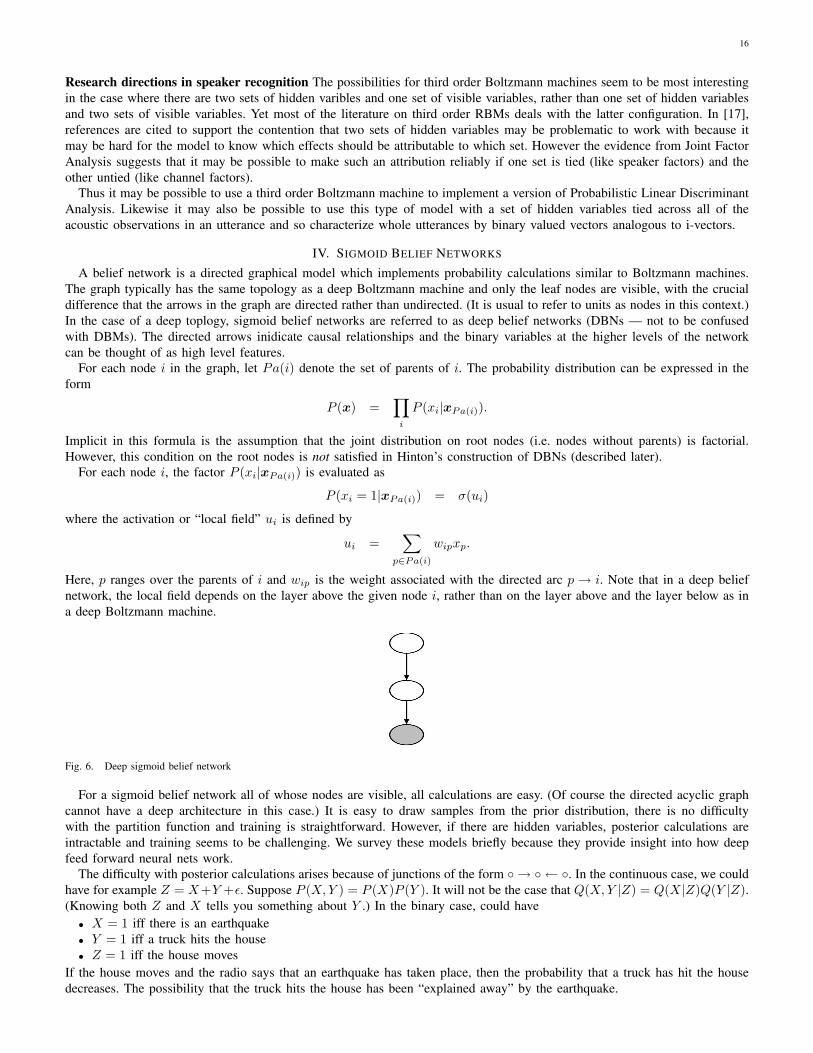
Fig. 6. Deep sigmoid belief network

For a sigmoid belief network all of whose nodes are visible, all calculations are easy. (Of course the directed acyclic graphcannot have a deep architecture in this case.) It is easy to draw samples from the prior distribution, there is no difficultywith the partition function and training is straightforward. However, if there are hidden variables, posterior calculations areintractable and training seems to be challenging. We survey these models briefly because they provide insight into how deepfeed forward neural nets work.

The difficulty with posterior calculations arises because of junctions of the form ◦ → ◦ ← ◦. In the continuous case, we couldhave for example Z = X+Y +ε. Suppose P (X,Y ) = P (X)P (Y ). It will not be the case that Q(X,Y |Z) = Q(X|Z)Q(Y |Z).(Knowing both Z and X tells you something about Y .) In the binary case, could have• X = 1 iff there is an earthquake• Y = 1 iff a truck hits the house• Z = 1 iff the house moves

If the house moves and the radio says that an earthquake has taken place, then the probability that a truck has hit the housedecreases. The possibility that the truck hits the house has been “explained away” by the earthquake.

17

A. TrainingWe assume to begin with that there are no hidden nodes. and derive the gradient of the log likelihood function. Note that

∂

∂wiplnP (x) =

∂

∂wiplnP (xi|xPa(i)).

Claim∂

∂wiplnP (xi|xPa(i)) = xpxi − xpσ(ui)

For, in the case xi = 1,∂

∂wiplnP (xi = 1|xPa(i)) =

∂ lnσ(ui)∂wip

= (1− σ(ui))xp

= xixp − σ(ui)xp if xi = 1

and in the case xi = 0,∂

∂wiplnP (xi = 0|xPa(i)) = − 1

P (xi = 0|xPa(i))∂σ(ui)∂wip

= − σ′(ui)1− σ(ui)

wip

= −σ(ui)xp

= xixp − σ(ui)xp if xi = 0.

Note that there is an analogy here with CD-1. Since σ(ui) can be interpreted as P (xi = 1|xPa(i)), we have the followingstochastic approximation

∂

∂wip

⟨lnP (xi|xPa(i))

⟩data

≈ xpxi − xpxi

where x is a stochastic reconstruction of x such that xi takes the value 1 with probability σ(ui).

B. Problem with Gibbs samplingThe stochastic gradient approximation can easily be extended in principle to the case there are hidden variables using Gibbs

sampling. (Given a training token v, draw a sample x from the posterior Q(x|v) and use it to build a 1-step reconstructionx.) But there is a problem in practice, namely that Gibbs sampling for sigmoid belief networks is computationally expensive,even if the directed acyclic graph has a deep architecture.

Consider variables at 3 levels hl+1,hl and hl−1. The distribution P (hl|hl+1) is factorial but the distribution Q(hl|hl+1,hl−1)is not because of explaining away. This means that the nodes at level l interfere with each other during Gibbs sampling. On theother hand in the case of a deep Boltzmann machine the distribution Q(hl|hl+1,hl−1) is factorial and there is no interference.

To calculate Q(xi|x\i) in a general directed acyclic graph, note that the factors in the prior P (x) which involve xi areP (xi|xPa(i)) and P (xj |xPa(j)) where i ∈ Pa(j) i.e. j ∈ C(i). Thus

Q(xi|x\i) ∝ P (xi|xPa(i))∏

j∈C(i)

P (xj |xPa(j)).

Other than i itself, the variables appearing in on the right hand side are of three types: the parents of i, the children of i andthe parents of the children of i. This collection of nodes is known as the Markov blanket of i. Denoting the Markov blanketby B(i), Q(xi|x\i) = Q(xi|xB(i)) [8].

In the case of a deep sigmoid belief net, the Markov blanket consists of the layer containing i, as well as the layer aboveand the layer below.

C. Variational BayesLikewise variational Bayes runs into trouble for deep belief networks.• As in the case of Gibbs sampling, a full factorization is needed. (The fixed point equations for each node involve the

variational parameters for all of the nodes in its Markov blanket, not just the nodes in the layer above and the layerbelow.)

• Even with a full factorization, the variational lower bound cannot be evaluated exactly and a cruder lower bound has tobe used.

• Since the EM auxiliary function is essentially the same as the variational lower bound, the EM algorithm cannot beimplemented exactly either.

See Section 11.12 of Haykin [9] for more information.

18

D. The wake sleep algorithm

Hinton has proposed a way of training deep sigmoid belief networks which attempts to circumvent the intractability of theposterior calculation. Recall that two ways of writing the EM auxiliary function are

〈lnP (v,h)〉+H(Q(h|v))lnP (v)− D (Q(h|v) || P (h|v)) .

To improve the fit of the model to a given data vector v, we can1) Hold the posterior Q(h|v) fixed and increase 〈lnP (x)〉 (where x is a short-hand for (h,v))2) Hold the model P (v) fixed and decrease the divergence between the true posterior P (h|v) and the approximate posterior

Q(h|v)and alternate between the two.

For 1), we need to evaluate the gradient with respect to the weight matrix of 〈lnP (x)〉. If we can sample from x ∼ Q(x|v),we can use the stochastic approximation

∂ 〈lnP (x)〉∂wip

≈ xpxi − xpxi

where x is a stochastic reconstruction of x. (This is the wake phase: the model is paying attention to what is going on in thereal world, namely the data vector v.)

The problem of sampling from the posterior is addressed by 2). Recall that sampling from the prior distribution of a deepbelief net is easy using the decomposition

P (x) =∏

i

P (xi|xPa(i))

and that training a deep belief net is easy if all of the needs are visible. For the sleep phase, assume that the posterior Q(x|v)can be approximated as

Q(x|v) =∏

i

Q(xi|xC(i)),

that is, by a sigmoid belief net with the arrows reversed. Thus the visible vectors form the input layer and, for each branchp→ i in the original graph with weight wip there is a branch i→ p in the dual graph with a different weight w′pi associatedwith it. The “visible” data used to train the dual deep belief network is obtained by sampling from the model, P (x), rather thanfrom the real world. (This is the sleep phase: the model is dreaming.) The weights wip are referred to as the generative weightsand the weights w′pi as the recognition weights; it is only the recognition weights that are used to evaluate the approximateposterior.

Suppose that we are given a training set {vn}, then the quantity that is being optimized in the wake phase is just∑n

∑h

Q(h|vn) lnP (h,vn)

which is exactly what is required by the EM algorithm. In the sleep phase, the model P (v,h) is fixed and a synthetic trainingset {vn,hn} is generated by sampling from the model. The quantity that is being optimized is the log likelihood of thissynthetic training set calculated with the dual deep belief net (thus the optimization is with respect to Q)∑

n

lnQ(hn|vn) =∑

n

∑h

P (h|vn) lnQ(h|vn)

≡ −∑

n

D (P (h|vn) ||Q(h|vn))

There are two problems with this: a synthetic training set rather than the real training set is being used and the optimandinvolves divergences of the form D (P (h|v) ||Q(h|v)), rather than D (Q(h|v) || P (h|v)) as required by the EM algorithm.

Unfortunately this elegant idea does not seem to work very well in practice [18]. Although they cannot be implemented onvery large scales, Gibbs sampling and variational Bayes perform better than wake-sleep training (you get what you pay for).

Mean field approximationThe adavantage of the wake-sleep algorithm is computational efficiency, particularly if the mean field approximation is used

to calculate approximate posteriors. Instead of propagating arrays of random binary vectors from the data layer up to the higherlayers, the mean field approximation propagates arrays of Bernoulli probablities. Sampling from the approximate posterior isthen just a matter of sampling independently from these Bernoulli distributions.

We use the superscript l to indicate variables associated with nodes at level l. Given a data vector v, set

Q(hli = 1|v) = µl

i

19

In the mean field approximation, µl+1j is calculated from the Bernoulli probabilities at level l using the recognition weights

on the branches joining level l to level l + 1

µl+1j = σ

(∑i

w′jiµli

).

Note that the mean field computation operates in the same way as a feed forward neural net, although the top layer of theneural net (the one that makes the recognition decisions) is missing.

To the extent that it is possible to train DBNs and carry out inference (that is, to do posterior calculations) with them,DBNs will be useful for constructing deep neural nets. Regarded as a generative model and trained in an unsupervised way,the variables at the higher levels of a DBN provide causal explanations of the data; inferring the values of these variables forgiven a data vector (using the recognition weights) can be regarded as extracting high level features from the data. Ideally,such high level features should prove more useful than the raw data vectors for recognizing patterns.

V. FEED FORWARD NEURAL NETS

A feed forward neural net consists of• A set of layers which implement the mean field posterior calculation for a DBN• A softmax layer for making recognition decisions

The activation ui for a node i is wTi x where x is the configuration of the layer underneath it. (This is the argument for the

sigmoid activation function, not the value returned by the activation function.)

For “label” nodes, σ is replaced by the softmax function. The probability assigned to the ith class label is

pi =eui∑j e

uj

The error signal associated with a training token is usually taken to be

E = −∑

i

ti ln pi

where the target value ti is 1 if i is the correct class label for the training token and 0 otherwise.

Fig. 7. Feed forward neural network

A. Backpropagation

Recall for any node i the activation ui is given by ui =∑

p wipxp where p ranges over the parents of i and the value takenby the node xi = σ(ui). (When we talk about parents in this context we are assuming that the arrows are directed as in Fig.7.) Suppose that ui and xi have been calculated for all nodes i in a forward pass. We explain how to calculate the derivatives

∂E∂wip

.

It is enough to calculate ∂E/∂ui since

∂E∂wip

=∂E∂ui

∂ui

∂wip

=∂E∂ui

xp.

To begin with, let i be node other than a label node, so that xi = σ(ui).∂E∂ui

=∂E∂xi

∂xi

∂ui

=∂E∂xi

σ′(ui)

20

and, since uj =∑

i wjixi,

∂E∂xi

=∑

j

∂E∂uj

∂uj

∂xi

=∑

j

wji∂E∂uj

so∂E∂ui

= σ′(ui)∑

j

wji∂E∂uj

.

Since wji is the weight associated with the branch i → j, wji = 0 and j contributes nothing to the sum on the right handside unless j is in the layer above i. Thus the calculation of the derivatives propagates in the backwards direction (from thelabels back to the data).

All that remains is to explain how to initialize the recursion. If i is a node in the softmax layer,

∂E∂ui

= −∑

k

tk∂

∂ui

uk − ln∑

j

euj

= −

∑k

tk

δik − 1∑j e

uj

∑j

eujδij

= −

∑k

tk (δik − pi)

= −(ti − pi).

B. Speech recognition with a neural net

Acoustic observation vectors represented as binary vectors or arrays of Bernoulli probabilities using a Gaussian-BernoulliRBM Universal Background Model can be used as input to a train a feed forward neural network for speech recognition.

Although in previous applications of neural nets to speech recognition the aim was to classify acoustic observation vectorsas phonemes (about 40 in all), Microsoft (most recently [7], and the references cited there) uses a different inventory consistingof a few thousand classes as in conventional speech recognizers. The idea is that the acoustic manifestation of a phonemedepends on the phonemes which precede and follow it through co-articulation effects. A naive approach to dealing with theco-articulation problem would be to model each phoneme-in-context with its own hidden Markov model (HMM). But, even ifonly the immediate left and right context of a phoneme is taken into account, the number of HMM output distributions to bemodeled would be prohibitively large. The standard way of dealing with this is to use a decision tree to cluster the number ofdistributions down to a manageable number (typically a few thousand) of “triphone states” or “senones”. Thus the role of theneural network then is to discriminate between a few thousand triphone states. Every acoustic observation in the training datais labelled as belonging to exactly one of these states by a forced Viterbi alignment. So training a feedforward neural networkto discriminate between the states is straightforward, to the extent that backpropagation can be relied on to work properly.

In order to use it in a Viterbi search in a speech recognizer, the posterior distribution P (c|v) produced by the neural shouldbe converted to generative form. This is trivial. By Bayes rule,

P (v|c) =P (c|v)P (v)

P (c).

The term P (c) can be estimated by counting state frequencies in the training data and the term P (v) can be ignored (sinceit is common to all classes). The distributions P (v|c) serve as the HMM output distributions in an otherwise conventional,single pass speech recognition architecture.

Compared with a conventional, single pass discriminatively trained approach (MMI-HMM) the neural net approach achieves30% error rate reductions on hard benchmarks (the Switchboard and Fisher conversational telephone speech corpora). Of coursestate of the art conventional systems are not single pass systems. (State of the art systems are adaptive, using provisionaltranscriptions of the data to be recognized to adjust the recognizer’s parameters. Multiple interations of adaptation may beperformed.) The performance of the single pass neural net system is about the same as that of a complex adaptive state-of-the-artsystem.

At this writing, no work seems to have been done on the problem of how a neural net speech recognition system might bemade adaptive. In a standard recognition system, most adaptation methods use a provisional transcription of the data (that is,a labeling of acoustic observations by triphone states) to adjust the generative output distributions P (v|c) so as to produce a

21

better match with the data. It is hard to guage how difficult adapting a discriminative neural net to a provisional transcriptionmight be.

It came as a surprise (not least to the Microsoft authors) that very good results could be achieved with unaided back-propagation, apparently starting from random initializations, Conventional wisdom has it that deep neural networks cannot betrained in this way in practice. (The authors suggest that discriminating between several thousand triphone states rather thanforty phonemes may explain their success. Even a single hidden layer produces very good results in this situation [14]. Theyalso point to the benefits of using a Gaussian-Bernoulli RBM which models feature vectors defined by concatenating cepstralfeatures extracted from blocks of 11 frames.) In fact, the authors’ starting point for training neural nets was the deep beliefnet construction to be described in the next section; only after the fact did they do due dilligence. They found that many ofthe excellent results they had originally obtained with the deep belief net construction could also be obtained without it. Thejury is still out on this.

VI. HINTON’S DEEP BELIEF NETWORKS

Fig. 8. Unfolding an RBM into a DBN

To motivate Hinton’s construction of deep Belief networks, observe that the models in Fig. 8 are all equivalent. For thesecond graph, the pair (h1,h2) is a mirror image of the pair (v,h1) in the first graph. For the third graph, the pair (h2,h3)is a mirror image of the pair (h1,h2) in the second graph.

Comparing the first and second graphs, the models are the same because P (v|h1) is the same in both cases and, by themirror image condition, P (h1) is the same in both cases:

P (h1) =∑

v

P (v)P (h1|v)

=∑h2

P (h2)P (h1|h2)

so P (v) is the same in both cases. Comparing the second and third graphs, the argument we have just given shows that P (h1)is the same in both cases; since P (v|h1) is the same in both cases, P (v) is the same in both cases. (This argument can beextended indefinitely, so that a restricted Boltzmann machine can be interpreted as an infinitely deep sigmoid belief network.)

For these arguments to be valid, the weight matrix for the original RBM has to be copied to all of the levels, but we obtaina more flexible class of models by allowing different weight matrices at different levels. It has become standard usage to referto models of this type as deep belief networks but this departs from traditional usage since the prior on the hidden variablesat the top level (e.g. h3) is not factorial.

A. Hinton’s construction

Given training data {vn}, Hinton and colleagues [19] show how addding successive levels to a DBN in the way just describedand calculating an approximate posterior on the hidden variables guarantees the variational lower bound increases everytime alevel is added. In the case of a model with l levels, the joint distribution of the hidden and visible variables and the approximateposterior of the hidden variables are given by

P (h1, . . . ,hl,v) = P (v|h1)P (h1|h2) . . . P (hl−2|hl−1)P (hl−1,hl)Q(h1, . . . ,hl|v) = Q(h1|v)Q(h2|h1) . . . Q(hl|hl−1). (1)

The probabilities P (v|h1), P (h1|h2), . . . , P (hl−2|hl−1) and the joint distribution P (hl−1,hl) can be calculated exactly usingthe RBM weight matrices at the various levels. The terms Q(h1|v), Q(h2|h1), . . . , Q(hl|hl−1) could also be calculated exactlyusing the RBM weight matrices but in practice a mean field approximation is used (as in the wake-sleep algorithm).

The weight matrix associated with level l+1 is estimated using the RBM training algorithm applied to an aggregated trainingset.2. That is, for each training token vn we sample from the posterior Q(hl|vn) and the collection of samples obtained in

2We encountered this type of synthetic data set in Section III-J

22

this way constitutes the training set for RBM training of the matrix at level l+ 1. Thus the hidden variables at one level serveas features for training the next.

Consider the case l = 1. Suppose that after training a first level RBM with weight matrix W 1 we wish to add a secondlevel. Construct a second RBM with weight matrix W 2 whose “visible” level is the hidden level of the first RBM and letP (h2|W 2) be the marginal distribution of the hidden level of the second RBM. Use the aggregated training set at level 1 andordinary RBM training to estimate W 2. The criterion which is optimized is∑

n

∑h1

lnP (vn,h1|W 1,W 2)

where h1 ranges over the aggregated training set. This is equivalent to optimizing the EM auxiliary function∑n

∑h1

Q(h1|vn,W 1) lnP (vn,h1|W 1,W 2)

which reduces to optimizing ∑n

∑h1

Q(h1|vn,W 1) lnP (h1|W 2)

since P (vn|h1,W 1,W 2) is independent of W 2. Here P (h1|W 2) is the marginal distribution calculated by regarding h1 asthe visible variables for the second RBM:

P (h1|W 2) =∑h2

P (h1,h2|W 2)

(Since the only part of the complete likelihood function P (v,h1) that is being re-estimated is the prior on the hidden variablesh1 so this is an instance of minimum divergence training.) We can initialize the RBM training of W 2 by copying W 1, soRBM training ensures that∑

n

∑h1

Q(h1|vn,W 1) lnP (h1|W 2) ≥∑

n

∑h1

Q(h1|vn,W 1) lnP (h1|W 1).

Of course this way of guaranteeing that the EM auxiliary function increases constrains the number of nodes added at level 2to be the same as the number of visible nodes at level 1. After adding the second level, the joint distribution of (v,h1,h2) is

P (v|h1,W 1)P (h1,h2|W 2)

where the first factor is calculated with the first RBM and the second with the second RBM. (Note the asymetry: one is aposterior distribution, the other a joint distribution.) The posterior of (h1,h2) given v, that is

P (v|h1,W 1)P (h1,h2|W 2)P (v)

,

cannot be calculated exactly so we use the approximation given by (1)

Q(h1,h2|v) = Q(h1|v)Q(h2|h2)

instead, where the first term is calculated with W 1 and the second with W 2. We must show that the variational lower boundat level 2 calculated with this posterior, L2, is greater than the variational lower bound calculated at level 1, L1.

By definition

L2 =∑

n

EQ(h1,h2|vn)

[lnP (vn,h1,h2)

]+∑

n

H(Q(h1,h2|vn)),

which we rewrite as follows

L2 =∑

n

EQ(h1,h2|vn)

[lnP (vn,h1,h2)

]+∑

n

H(Q(h1,h2|vn))

=∑

n

EQ(h1,h2|vn)

[lnQ(h2|h1) + lnP (vn,h1)

]+∑

n

H(Q(h1,h2|vn))

=∑

n

∑h1,h2

Q(h1,h2|vn) lnQ(h2|h1) +∑

n

∑h1

Q(h1|vn) lnP (vn|h1)P (h1|W 2)

−∑

n

∑h1,h2

Q(h1,h2|vn)(lnQ(h2|h1) + lnQ(h1|vn)

)=

∑n

∑h1

Q(h1|vn) lnP (vn|h1)P (h1|W 2) +∑

n

H(Q(h1|vn)).

23

On the other hand,

L1 =∑

n

∑h1

Q(h1|vn) lnP (vn,h1|W 1) +∑

n

H(Q(h1|vn))

=∑

n

∑h1

Q(h1|vn) lnP (vn|h1)P (h1|W 1) +∑

n

H(Q(h1|vn)).

and the inequality L2 ≥ L1 follows from the fact that W 2 was chosen so that∑n

∑h1

Q(h1|vn) lnP (vn|h1)P (h1|W 2) ≥∑

n

∑h1

Q(h1|vn) lnP (vn|h1)P (h1|W 1).

Fig. 9. Standard deep belief net, Hinton deep belief net, deep Boltzmann machine and feed forward neural net

Note The posterior approximation (1) is not as good as it might be because the way that a term such as Q(hk|hk−1) isevaluated depends on the construction up to level k but not on the construction of subsequent levels. On the other hand thevariational Bayes posterior calculation used in training deep Boltzmann machines takes account of all levels above and belowin evaluating the posterior at a given level k.

The argument that the variational lower bound increases as successive layers are added to a DBN requires that the weightmatrices have the same dimensions at all levels; there is no such restriction for DBMs. Also the DBN level building algorithmis inherently greedy, but the DBM training algorithm is not (although it may have to be initialized greedily in practice, aprocess commonly referred to as pretraining).

Generative pattern recognition In [19], the authors show how, after building a multilayer DBN in the way just described aslight modification of the wake-sleep algorithm can be used to improve it. As in the case of traditional deep belief networks,each weight matrix (expect for the weight matrix which defines the top layer RBM) is a replaced by a pair of matrices, oneof which is used to calculate posteriors and the other to sample from the generative model.

By adding a softmax layer with 10 label nodes, the DBN can serve as a generative model of label-image pairs in the MNISThandwritten digit data set. The model can be used to recognize digits using the minimum Bayes risk principle (that is, bycalculating posteriors of the form P (label|digit)). At the time of publication, results on the MNIST test set obtained in thisway were state of the art.

Discriminative pattern recognition Suppose we have built a DBN with L levels, so that the calculation of Q(hL|v) using themean field approximation (1) mimics the activity of a feed forward neural net (without the softmax layer). The generative modelis trained in an unsupervised way (without class labels) but we assume that training behaves in such a way that the highestlevel hidden variables are the most useful features for discriminating between classes. Thus we can assume a decompositionof the form

Q(c|v) =∑hL

Q(c|hL)Q(hL|v)

where c denotes a class label vector and Q(c|hL) is calculated with a softmax layer. Most of the parameters in this neuralnetwork (namely those which specify Q(hL|v)) are derived from the generative model of the data. The backpropagationalgorithm is very successful if initialized from the generative model in this way. This seems to have come as something of asurprise to the machine learning community as it had long been argued that one should not pay much attention to the termP (v) in the decomposition

P (v, c) = Q(c|v)P (v)

since P (v) (that is, the generative model) plays no direct role in recognition decisions.The success of generative modeling as an initialization for backpropagatation is attributed to the fact that, if left to its own

devices, backpropagation generally gets stuck in a local minimum of the error function or overfits the training data. (Hintonfrequently argues that generative modeling is less susceptible to overfitting than discriminative modeling.) See Section 4 of [1]for a discussion of these questions.

24

B. DBNs vs DBMs

Salakhutdinov suggests that Hinton’s construction can be used with a minor modification to initialize deep Boltzmannmachines [2].

Consider the case l = 2. The joint distribution of the hidden and visible variables in a 2 layer DBN is

P (v,h1,h2) = P (v|h1,W 1)P (h1,h2|W 2)

which is not a Boltzmann distribution. If we were to take the product

P (v,h1|W 1)P (h1,h2|W 2)

and normalize the probabilities so that they sum to 1, we would get a Boltzmann distribution but this expression counts theprior on h1 twice. (The first and second level RBMs each contribute a prior on h1.) To avoid this doubling effect Salakhudtinovsuggests halving the weight matrices W 1 and W 2 before taking the product and renormalizing. The higher levels are handledin the same way. This heuristic is merely used an initialization for subsequent DBM training.

It appears that, when used as feature extractors for discriminative pattern recognition, DBMs outperform DBNs [2] but moreresearch seems to be needed here. Training DBMs is much slower than training DBNs becasue the variational Bayes posteriorcalculation for DBMs is more computationally demanding than the mean field approximation used to evaluate posteriors forDBNs. The variational Bayes posterior calculation requires cycling over all of the levels in the DBM rather than performinga single feed forward pass. This results in a better posterior calculation but, contrary to the case of DBNs, it does not suggestan immediately obvious way of using the DBM weight matrix to initialize a feed forward neural network for discriminativepattern recognition. Salakhutdinov proposes such an initialization in the case of a DBM with two hidden layers but it is notclear to me how this would extend to the case of three hidden layers.

VII. SOME RESEARCH PROBLEMS FOR BOLTZMANN MACHINES

Although the DBM training algorithm appears to be better than the DBN training algorithm because sparse Boltzmannmachines support efficient variational Bayes inference, only Salakhutdinov appears to have explored using DBMs in buildingdiscriminative closed-set pattern recognizers in a similar manner to DBNs and, as discussed above, Salakhutdinov’s solutionappears to be incomplete.

Although interest in DBNs was revived by the way they were used to build a a generative pattern recognizer in Hinton,Osindero and Teh [19], very little work seems to have been done on using DBMs for generative pattern recognition. Of coursea straightforward approach to building generative pattern recognizers using BMs would be to construct a separate generativemodel for each class to be recognized but this seems to be less interesting than the approach of designing a single generativemodel to recognize all classes as in [19]. Ideally, a single generative model constructed in this way should lend itself to beingturned into a (presumably better) discriminative pattern recognizer. Moreover, when applied to speech recognition, it should becapable of accommodating utterance level hidden variables which could serve to characterize the speaker and channel effectsin a given recording. Estimating these hidden variables for a given utterance would enable speech recognition to be carriedout in a speaker adaptive way.

An easier way of designing a speaker adaptive neural net speech recognizer might be to use traditional feature spacetransformation methods such as fMLLR. This would decouple the problem of estimating utterance level hidden variables fromthat of training the neural net. Accommodating utterance level hidden variables in a triphone state recognizer trained withbackpropagation does not seem to be easy but the general problem of how to integrate utterance level hidden variables into adiscriminative speech recognizer looks interesting.

A. Generative pattern recognition

We have seen how variables of different types (binary and real-valued) can be jointly modeled in the Gauss-Bernoulli RBM.Note that it is not the case that the marginal distribution of the real-valued variables is Gaussian; rather the conditional of eachreal-valued valued variable given all of the other variables is Gaussian. This observation indicates how Boltzmann machinescan be extended to accommodate other types of distribution.

The “exponential family harmonium” (Welling et al.) is a generalization where the nodes in the graph have associatedwith them variables which may be discrete (binary or categorical) or continous (scalar or vector valued) and the conditionaldistribution of one variable given the others is in the exponential family. Different types of exponential distribution can beaccomodated in a single model. All of the VBEM and contrastive divergence training algorithms can be extended to theharmonium (I think). Because categorical variables are supported generative models for N -way pattern recognition (as distinctfrom 2-way pattern recognition) can be built (although this doesn’t seeem to have been explored widely).

Because this type pattern recognizer is a generative model, it should not be hard to introduce utterance level hidden variablesfor speech recognition applications. All that would be required would be to designate some of the hidden variables as beingtied across all of the acoustic observations in a given utterance.

25

B. Discriminative pattern recognition

To fix ideas suppose we have built a generative BM pattern recognizer with 2 visible layers (one for data, the other for labels)and 4 hidden layers and that 3 iterations of variational Bayes are needed to perform pattern recognition. The 3 variationalBayes iterations can be unfolded into 15 (i.e. 3× 4) mean field updates; that is, they can be implemented by a 15 layer feedforward neural net with tied weight matrices. Standard backpropagation could be used to untie and re-estimate the weightmatrices, converting the generative pattern recognizer into a discriminative pattern recognizer. (Perhaps the label layer oughtto be handled differently, for instance as in [2].)

If the generative pattern recognizer is designed so as to contain utterance level hidden variables the same would be true ofthe discriminative pattern recognizer.

REFERENCES

[1] Y. Bengio, “Learning deep architectures for AI,” Foundations and Trends in Machine Learning, vol. 2, no. 1, pp. 1–127, 2009.[2] R. Salakhutdinov and G. Hinton, “An efficient learning procedure for deep boltzmann machines,” in CSAIL Technical report, MIT-CSAIL-TR-2010-37,

Aug. 2010.[3] D. MacKay, Information theory, inference and learning algorithms. New York, NY: Cambridge University Press, 2003.[4] P. Kenny, P. Ouellet, N. Dehak, V. Gupta, and P. Dumouchel, “A study of inter-speaker variability in speaker verification,” IEEE Trans. Audio, Speech

and Lang. Process., vol. 16, no. 5, pp. 980–988, July 2008. [Online]. Available: http://www.crim.ca/perso/patrick.kenny[5] N. Dehak, P. Kenny, R. Dehak, P. Dumouchel, and P. Ouellet, “Front-end factor analysis for speaker verification,” IEEE Trans. Audio, Speech, Lang.

Process., vol. 19, no. 4, pp. 788–798, May 2011.[6] P. Kenny, “Bayesian speaker verification with heavy tailed priors,” in Proc. Odyssey 2010: The speaker and Language Recognition Workshop, Brno,

Czech Rebublic, June 2010.[7] F. Seide, G. Li, and D. Yu, “Conversational speech transcription using context-dependent deep neural networks,” in Proc. Eurospeech 2011, 2011.[8] C. Bishop, Pattern Recognition and Machine Learning. New York, NY: Springer Science+Business Media, LLC, 2006.[9] S. Haykin, Neural networks: a comprehensive introduction. Upper Saddle River, New Jersey: Prentice-Hall, Inc., 1999.

[10] Y. Bengio and O. Delalleau, “Justifying and generalizing contrastive divergence,” Neural Computation, vol. 21, no. 6, pp. 1601–1621, 2009.[11] K. Cho, A. Ilin, and T. Raiko, “Improved learning of Gaussian-Bernoulli restricted Boltzmann machines,” in Master’s Thesis, Aalto University, 2011.[12] G. Dahl and G. Hinton, “Phone recognition with the mean-covariance restricted boltzmann machine,” in Advances in Neural Information Processing 23,

2010.[13] A. Mohammed, G. Dahl, and G. Hinton, “Acoustic modeling using deep belief networks,” IEEE Trans. on Audio, Speech, and Language Processing,

2010.[14] G. Dahl, D. Yu, L. Deng, and A. Acero, “Context-dependent pre-trained deep neural networks for large vocabulary speech recognition,” IEEE Transactions

on Audio, Speech, and Language Processing (Special Issue on Deep Learning for Speech and Language Processing), Jan. 2012.[15] A. Mohammed, T. Sainath, G. Dahl, B. Ramabhadran, G. Hinton, and M. Picheny, “Deep belief networks using discriminative features for phone

recognition,” in Proc. ICASSP 2011, 2011.[16] G. Dahl, D. Yu, L. Deng, and A. Acero, “Context-dependent pre-trained deep neural networks for large vocabulary speech recognition,” in Advances in

Neural Information Processing 23 .[17] R. Memisevic and G. Hinton, “Learning to represent spatial transformations with factored higher-order Boltzmann machines,” Neural Computation,

vol. 22, pp. 1473–1492.[18] B. Frey, G. Hinton, and P. Dayan, “Does the wake-sleep algorithm produce good density estimators?” in Advances in Neural Information Processing 8,

1996.[19] G. Hinton, S. Osindero, and Y. Teh, “A fast learning algorithm for deep belief nets,” Neural Computation, vol. 18, pp. 1527–1554, 2006.