1

Nonparametric Methods II

Henry Horng-Shing LuInstitute of Statistics

National Chiao Tung Universityhslu@stat.nctu.edu.tw

http://tigpbp.iis.sinica.edu.tw/courses.htm

2

PART 3: Statistical Inference by Bootstrap Methods

References Pros and Cons Bootstrap Confidence Intervals Bootstrap Tests

3

References Efron, B. (1979). "Bootstrap Methods: Another

Look at the Jackknife". The Annals of Statistics 7 (1): 1–26.

Efron, B.; Tibshirani, R. (1993). An Introduction to the Bootstrap. Chapman & Hall/CRC.

Chernick, M. R. (1999). Bootstrap Methods, A practitioner's guide. Wiley Series in Probability and Statistics.

4

Pros (1) In statistics, bootstrapping is a modern,

computer-intensive, general purpose approach to statistical inference, falling within a broader class of re-sampling methods.

http://en.wikipedia.org/wiki/Bootstrapping_(statistics)

5

Pros (2) The advantage of bootstrapping over

analytical method is its great simplicity - it is straightforward to apply the bootstrap to derive estimates of standard errors and confidence intervals for complex estimators of complex parameters of the distribution, such as percentile points, proportions, odds ratio, and correlation coefficients.

http://en.wikipedia.org/wiki/Bootstrapping_(statistics)

6

Cons The disadvantage of bootstrapping is that whil

e (under some conditions) it is asymptotically consistent, it does not provide general finite sample guarantees, and has a tendency to be overly optimistic.

http://en.wikipedia.org/wiki/Bootstrapping_(statistics)

7

How many bootstrap samples is enough?

As a general guideline, 1000 samples is often enough for a first look. However, if the results really matter, as many samples as is reasonable given available computing power and time should be used.

http://en.wikipedia.org/wiki/Bootstrapping_(statistics)

8

Bootstrap Confidence Intervals1. A Simple Method2. Transformation Methods

2.1. The Percentile Method2.2. The BC Percentile Method2.3. The BCa Percentile Method2.4. The ABC Method (See the book: An Introductio

n to the Bootstrap.)

9

1. A Simple Method Methodology Flowchart R codes C codes

10

Normal Distributions

2 21 2

2

1/ 2 / 2 / 2

/ 2 / 2

, , ..., ~ ( , ), is known.

ˆˆ ~ ( , ), ~ (0, 1).

/ˆ

( ) 1 (1 / 2)/

ˆ ˆ( / / ) 1

iid

n

LCL UCL

X X X N

X N Z Nn n

P z z where Zn

P z n z n

11

1 2

/ 2 / 2ˆ

ˆ ˆ/ 2 / 2

More generally,

, , ..., ~ ( ).

ˆLet , then

ˆ(0, 1).

ˆ. .( )

ˆ( ) 1

ˆ ˆ( ) 1

iid

n

n

n

X X X F x

MLE

Pivot Ns e

P z z

P z z

Asymptotic C. I. for The MLE

http://en.wikipedia.org/wiki/Pivotal_quantity

12

When is not large, we can construct

more precise confidence intervals

by bootstrap methods for many statistics

including the and others.

n

MLE

Bootstrap Confidence Intervals

13

*1

* * **

( ) (1 )2 2

Theorem in Gill (1989): Under regular conditions,

ˆn ( ( )) ( ) ,

ˆ ˆn ( ) ,..., ( ) .

Want 1

ˆ ˆ ˆ ˆ ˆ ˆNote that 1

on

on n

F d F B F

X X d F B F

P LCL UCL

P

* *

( ) (1 )2 2

* *

(1 ) ( )2 2

ˆ ˆ ˆ ˆ ˆ

ˆ ˆ ˆ ˆ 2 2

.

P

P

P LCL UCL

Simple Methods

14

11 2 101

1(1) (2) (101) (51)

1 2 101

* * *(1) (2) (101)

* * 1 *(51)

1, , ..., ~ ( , 1), = ( ).

21ˆ ... , ( ) .2

Resampling with replacement from , , ..., .

... .

1ˆ ( ) .2

Repeat 1000

n

n

X X X N median F

X X X F X

X X X

X X X

F X

B

* * *(1) (2) (1000)

times,

ˆ ˆ ˆwe can get ... .

An Example by The Simple Method (1)

15

* * ** (25) (975)

* * ** (25) (975)

* *(25) (975)

* *(975) (25)

* *(975) (25)

ˆ ˆ ˆ 1 95%

ˆ ˆ ˆ ˆ ˆ ˆ

ˆ ˆ ˆ ˆ ˆ

ˆ ˆ ˆ ˆ2 2 .

ˆ ˆ ˆ ˆ[ 2 , 2 ]

is an approximate (1- ) confidence in

P

P

P

P

LCL UCL

terval for .

*(1)̂ *

(1000)̂*(25)̂ *

(975)̂

95%

An Example by The Simple Method (2)

16

Flowchart of The Simple Method

*2x

*Bx

*(2)̂

1 2ˆ ( , , ..., ) ( )ndata x x x s x x

* *ˆget resample statistics ( ) and then sort themb bs x

*1x

resample B times

*(1)̂

100(1 )% confidence interval

1 2[( 1) / 2], [( 1)(1 / 2)]v B v B

2 1

* *( ) ( )

ˆ ˆ ˆ ˆ2 , 2v vLCL UCL

*( )ˆ

B*(2)̂

17

The Simple Method by R

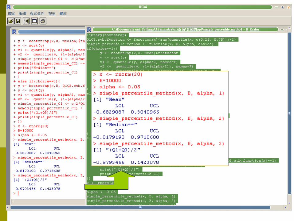
18

19

resample B times:

* *ˆ ( )b bmean x

*bx

The Simple Method by C (1)

ˆ ( ) ( )a s x mean x

20

The Simple Method by C (2)

calculate v1, v2

100(1 )% confidence interval

21

22

23

24

2. Transformation Methods 2.1. The Percentile Method 2.2. The BC Percentile Method 2.3. The BCa Percentile Method

25

2.1. The Percentile Method Methodology Flowchart R codes C codes

26

The Percentile Method (1) The interval between the 2.5% and 97.5%

percentiles of the bootstrap distribution of a statistic is a 95% bootstrap percentile confidence interval for the corresponding parameter. Use this method when the bootstrap estimate of bias is small.

http://bcs.whfreeman.com/ips5e/content/cat_080/pdf/moore14.pdf

27

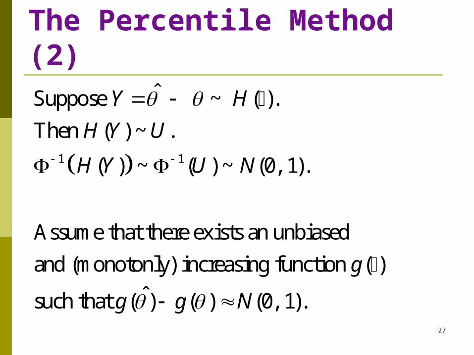
1 1

ˆSuppose ~ ( ).

Then ( ) ~ .

( ) ~ ( ) ~ (0, 1).

Assume that there exists an unbiased

and (monotonly) increasing function ( )

ˆsuch that ( ) ( ) (0, 1).

Y H

H Y U

H Y U N

g

g g N

The Percentile Method (2)

28

*

**

* 1 ** ([( 1)(1 )])

11

ˆIf ( ) ( ) (0, 1),

ˆ ˆthen ( ) ( ) (0, 1).

ˆ ˆ( ) ( ) 1

ˆ ˆ ˆ ˆ ( ( ) )) and

ˆ( ) ( )

ˆ ( ( ) )) (Note: for (0, 1

B

g g N

g g N

P g g z

P g g z

P g g z

P g g z z z N

1

1 *1 1 ([( 1) ])

).)

ˆ ˆ ˆ ( ( ) )) and .BP g g z

The Percentile Method (3)

29

*([( 1)(1 )])

* *([( 1) /2]) ([( 1)(1 /2)])

ˆ, 1

ˆ ˆ 1 .

B

B B

Similarly P

and P

*([( 1) ])

*([( 1)(1 )])

* *([( 1) /2]) ([( 1)(1 /2)])

Summary of the percentile method:

ˆ 1 ,

ˆ 1 ,

ˆ ˆ 1 .

B

B

B B

P

P

P

The Percentile Method (4)

30

Flowchart of The Percentile Method

*2x

*Bx

*(2)̂

1 2ˆ ( , , ..., ) ( )ndata x x x s x x

* *ˆget resample statistics ( ) and then sort themb bs x

*1x

resample B times

*(1)̂

100(1 )% confidence interval

1 2[( 1) / 2], [( 1)(1 / 2)]v B v B

1 2

* *( ) ( )ˆ ˆ,v vLCL UCL

*( )ˆ

B*(2)̂

31

The Percentile Method by R

32

33

The Percentile Method by C

*bx

calculate v1, v2

100(1 )% confidence interval

resample B times:

* *ˆ ( )b bmean x

34

35

36

37

2.2. The BC Percentile Method Methodology Flowchart R code

38

The BC Percentile Method Stands for the bias-corrected percentile meth

od. This is a special case of the BCa percentile method which will be explained more later.

39

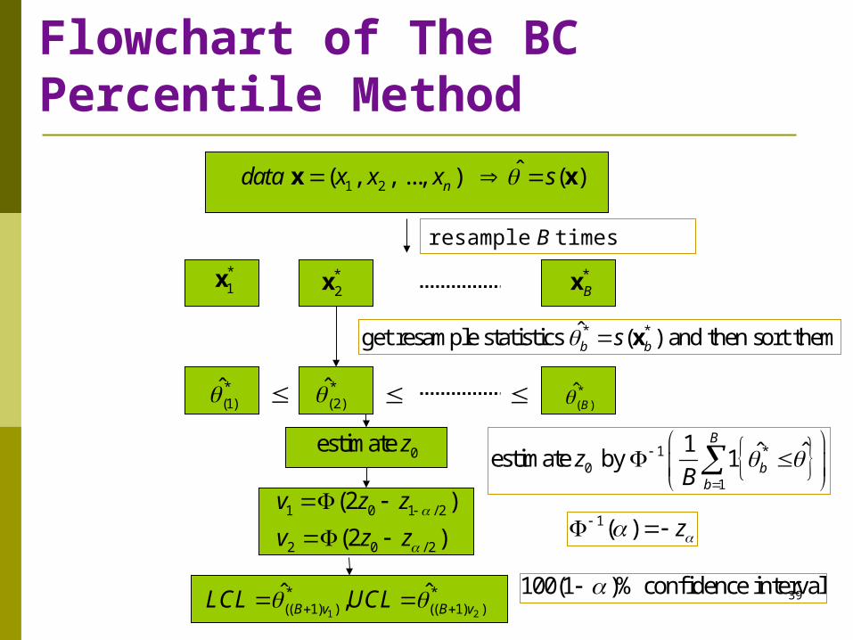
Flowchart of The BC Percentile Method

100(1 )% confidence interval

1 0 1 / 2

2 0 / 2

(2 )

(2 )

v z z

v z z

1 2

* *(( 1) ) (( 1) )ˆ ˆ,B v B vLCL UCL

0estimate z 1 *0

1

1 ˆ ˆestimate by 1B

bb

zB

*2x

*Bx

*(2)̂

1 2ˆ ( , , ..., ) ( )ndata x x x s x x

* *ˆget resample statistics ( ) and then sort themb bs x

*1x

resample B times

*(1)̂ *

( )ˆ

B*(2)̂

1( ) z

40

The BC Percentile Method by R

41

42

2.3. The BCa Percentile Method Methodology Flowchart R code C code

43

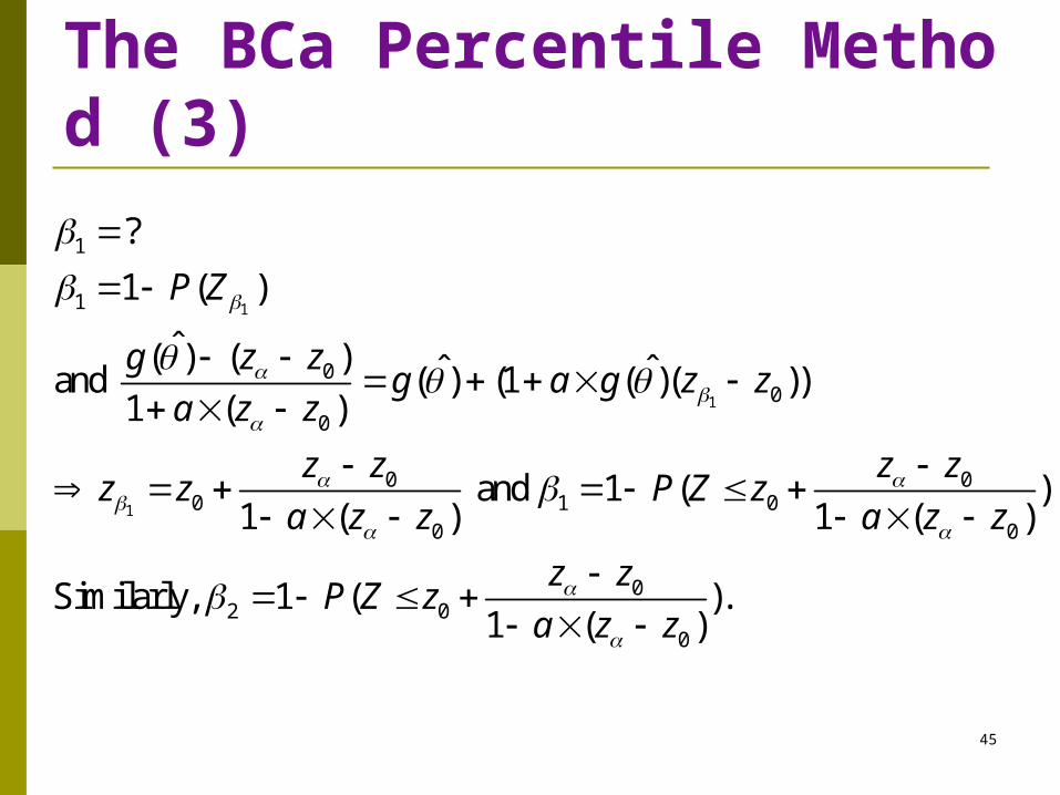
The BCa Percentile Method (1) The bootstrap bias-corrected accelerated (B

Ca) interval is a modification of the percentile method that adjusts the percentiles to correct for bias and skewness.

http://bcs.whfreeman.com/ips5e/content/cat_080/pdf/moore14.pdf

44

1

**

* 0

* 1 ** 0 *

0

1 0

0

1

ˆ ˆ( ) ( )1

ˆ1 ( )

ˆ ˆ ˆ ˆ( ( ) (1 ( ))( ) ) .

ˆ( ) ( )1

1 ( )

ˆ( ) ( )( )1 ( )

ˆ ˆ( ( ) (1 ( ))(

g gP U z z

a g

P g g a g z z P

g gP U z z

a g

g z zP g

a z z

P g g a g z

1

1 1

2

1 2

0

*([( 1) (1 )])

*([( 1) (1 )])

* *([( 1) (1 )]) ([( 1) (1 )])

) ) .

ˆ ˆ .

ˆSimilarly, ( ) 1

ˆ ˆand ( ) 1 2 .

B

B

B B

z P

P

P

The BCa Percentile Method (2)

45

1

1

1

1

1

00

0

0 00 1 0

0 0

02 0

0

?

1 ( )

ˆ( ) ( ) ˆ ˆand ( ) (1 ( )( ))1 ( )

and 1 ( )1 ( ) 1 ( )

Similarly, 1 ( ).1 ( )

P Z

g z zg a g z z

a z z

z z z zz z P Z z

a z z a z z

z zP Z z

a z z

The BCa Percentile Method (3)

46

0

* ** *

*

* 0 0

0

1 *0 *

1 *0

1

?

ˆ ˆ ˆ ˆ( ) ( ) ( )

ˆ ˆ ˆ ˆ( ) ( ) ( ) ( )

ˆ ˆ1 ( ) 1 ( )

( )

ˆ ˆ( ) and

1 ˆ ˆˆ 1 .B

bb

z

P P g g

g g g gP z z

a g a g

z

z P

zB

The BCa Percentile Method (4)

47

3( ) ( )

1

2 3/ 2( ) ( )

1

( ) 1, 1

?

ˆ ˆ( )ˆ ,

ˆ ˆ6 ( ( ) )

ˆwhere ( ) ({ , ...,

n

ii

Jack n

ii

i n i i

a

a

F X X

n

( ) ( )1

, ..., })

1ˆ ˆ .n

ii

X

andn

The BCa Percentile Method (5)

48

Flowchart of The BCa Percentile Method

/ 2 0 1 / 2 01 0 2 0

/ 2 0 1 / 2 0

1 ( ), 1 ( )1 ( ) 1 ( )

z z z zz z

a z z a z z

100(1 )% confidence interval1 2

* *(( 1) (1 )) (( 1) (1 ))ˆ ˆ,B BLCL UCL

0estimate , z a

*2x

*Bx

*(2)̂

1 2ˆ ( , , ..., ) ( )ndata x x x s x x

* *ˆget resample statistics ( ) and then sort themb bs x

*1x

resample B times

*(1)̂ *

( )ˆ

B*(2)̂

1 *0

1

1 ˆ ˆestimate by 1 and by JackknifeB

bb

z aB

1( ) z

49

Step 1: Install the library

of bootstrap in R.Step 2: If you want to check

BCa, type “?bcanon”.

50

51

The BCa Percentile Method by R

52

53

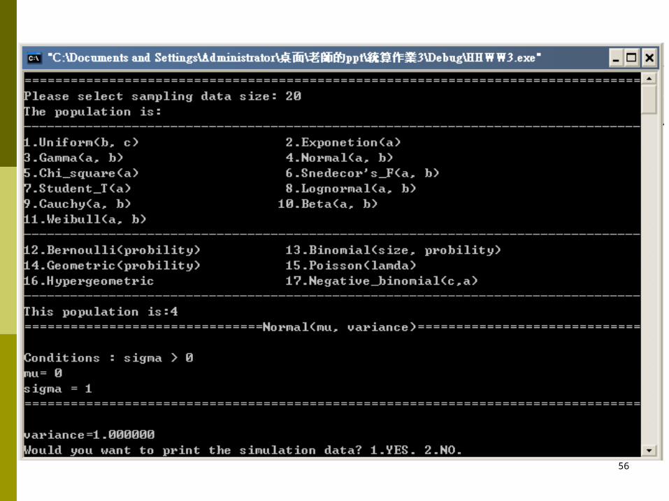
The BCa Percentile Method by C

54

55

56

57

58

59

Exercises Write your own programs similar to those

examples presented in this talk.

Write programs for those examples mentioned at the reference web pages.

Write programs for the other examples that you know.

Prove those theoretical statements in this talk.

59