Pragya the best FRM revision course!

FRM 2017 Part 2

Book 1 – Market Risk Measurement & Management

Pragya the best FRM revision course!

ESTIMATING MARKET RISK MEASURES

Reading: Estimating Market Risk Measures (Chapter 3, Kevin Dowd, Measuring Market Risk, 2nd Edition (West Sussex,

England: John Wiley & Sons, 2005))

1. Definitions:

a. Arithmetic Return: Pt+Dt − Pt−1

Pt−1 and Geometric Return: ln ቂ

Pt+Dt

Pt−1ቃ

b. Geometric return assumes that all money received is continuously reinvested at the same rate of return.

Also, it ensures that asset prices can never become negative

2. VaR using Historical Simulation: Order all daily return observations from largest to smallest. The observation

that comes after the threshold limit is the VaR (α.n)+1

3. Parametric Estimation of VaR:

a. Delta-Normal VaR: -µ + zσ [For 5% significance, Z is 1.65 and for 1% is 2.33]

b. Lognormal VaR: 1 – e (µ - zσ)

4. Q-Q Plots: It plots both the empirical and hypothesized distribution. If the two distributions are very

similar, then the plot will be linear

5. Standard Error: Used to assess the precision of the risk measure. The simplest method is to create a confidence

interval around the quantile in question.

a. Confidence Interval: z + (z. Std Error) > VaR > z - (z. Std Error)

b. f(q) is the area of a bin width

c. Std. Error = ඥp(1−p)/n

f(q)

6. Note:

a. Concepts like ES(Expected Shortfall) are carried forward from Part 1

b. Remember that VaR is one tailed and Confidence intervals are 2 tailed

NON-PARAMETRIC APPROACHES

Reading: Estimating Market Risk Measures (Chapter 4, Kevin Dowd, Measuring Market Risk, 2nd Edition (West Sussex,

England: John Wiley & Sons, 2005))

1. Definitions:

a. Surrogate Density Function: Curve obtained by connecting mid-points of successive histograms. Helps

calculate VaR at any percentage point.

2. Bootstrap Historical Simulation:

a. Draw a sample from the data set and estimate VaR

b. Put the data back in the data set.

c. Repeat step a and b multiple times. Best estimate of VaR is the average VaR of the simulation runs

3. Weighted Historical Simulation Approaches

a. Age-weighted: More recent observations have more weight. Weight is given by wi = λi−1 (1−λ)

1−λn

b. Volatility-weighted: 𝑟𝑡,𝑖∗ = 𝑟𝑡,𝑖

𝜎𝑇,𝑖

𝜎𝑡,𝑖

c. Correlation-weighted: Incorporates updated correlations between asset pairs

d. Filtered historical simulation: Volatility is forecast for each day in the sample period and bootstrapping

used for returns

4. Advantages of non-parametric approaches:

a. Computationally simple

b. Not hindered by parametric violations of skewness and fat tails

c. Can accommodate more complex analysis

5. Disadvantages of non-parametric approaches:

a. Analysis depends critically on historical data

b. Difficult to detect structural shifts

c. Need sufficient data

BACK TESTING VAR

Reading: Backtesting VaR (Chapter 6, Philippe Jorion, Value-at-Risk: The New Benchmark for Managing

Financial Risk, 3rd Edition(New York: McGraw Hill, 2007))

1. Backtesting: It is the process of comparing losses predicted by the VaR model to those actually

experienced over the testing period. An unbiased measure of the number of exceptions as a

proportion of the number of samples is called failure rate

a. Failure Rate = N

T where N is no. of exception and T is no. of samples

2. Error Types:

a. Type 1 Error: Rejecting an accurate model

b. Type 2 Error: Accepting an inaccurate model

3. Log-likelihood Ratio: LRuc is a test statistic to determine the hypothesis that model is accurate.

If LRuc > 3.84, we reject the hypothesis that the model is correct

a. As VaR confidence level increases, extreme values decrease. Thus, it becomes difficult to

test for the accuracy of the model

4. VaR to measure potential losses: To decide on the holding period, we have two theories.

a. Holding period should be equal to the amount of time required to either liquidate or

hedge the portfolio

b. It should match the period over which the portfolio is not expected to change

5. Basel Committee on Backtesting: Basel requires that Market VaR be computed at 99%

confidence interval and backtested for past 1 year.

a. We expect to have 2.5 exceptions (250x0.01) each year.

b. Depending on the exceptions observed, the capital multiplier (amount a bank must

hold) increases and this lowers the bank performance if model used is incorrect

i. Multiplier is 3 for Green zones (0-4 observations)

ii. Multiplier increases from 3-4 for yellow zone(5-9 observations)

iii. Multiplier is 4 for Red zone(more than 10 observations)

c. Multiplier is based on the type of model error

i. Basic Integrity lacking/ Model Inaccuracy then penalty applies

ii. Intraday trading then penalty may be considered

iii. Bad luck due to significant market conditions may be condoned

d. Reducing confidence interval reduces the probability of type 2 errors. Also, using longer

backtesting periods can help here

6. Conditional Coverage: Unconditional coverage does not test for timing of exceptions and

assumes that exceptions are fairly equally distributed across time. Conditional coverage includes

a measure of independence of the events i.e. LRcc = LRuc+ LRind thus, if LRcc > 5.99, we reject

the model

a. If exceptions are determined to be serially dependent, then model needs to be revised

to incorporate the correlations that are evident in current conditions.

VAR MAPPING

Reading: VaR Mapping (Chapter 11, Philippe Jorion, Value-at-Risk: The New Benchmark for Managing Financial Risk, 3rd

Edition (New York: McGraw Hill, 2007))

1. Mapping a Portfolio:

a. Market risk is measured by noting all the current positions within a portfolio. These positions are then

mapped to risk factors using factor exposures

b. Mapping involves finding common risk factors among positions in a given portfolio. This system is

position based and differs from the traditional return analysis

2. Factor Exposures:

Type Risk Factor Factor Exposure

Fixed Income Change in Interest rate Modified Duration

Equities Change in equity index prices Beta

a. If all positions in a portfolio are exposed to the same risk factors, the portfolio factor exposure can

be found as weighted average of position factor exposures

3. General and Specific Risks: One or two risk factors are appropriate to capture General or primitive risks. The

type and no. of risk factors will have an effect on the size of the residual or specific risks. Specific risks arise from

unsystematic risks of various positions in the portfolio. Diversification of the portfolio reduces specific risk and

only market risk remains (Systematic Risk or Beta)

4. Mapping Fixed Income Securities:

a. Principal Mapping: Risk of repayment of principal amounts. Average maturity of portfolio is mapped to

the coupon bond

b. Duration Mapping: Risk of bond is mapped to a zero coupon bond of the same duration. Risk level of

zero coupon bond equals the duration of the portfolio

c. Cash Flow Mapping: Risk of bond is decomposed into the risk of each cash flow of bond

d. If we assume perfect correlation between the maturity of the zeros, the portfolio VaR would be equal to

the undiversified VaR

5. Tracking error VaR: It is the deviation between the benchmark VaR and the portfolio VaR

6. Mapping for Linear Derivatives: The Delta-Normal method provides accurate estimates of VaR for portfolio and

assets that can be expressed as linear combinations of normally distributed risk factors e.g. Forwards.

7. Mapping for non-linear derivatives: Delta-Normal cannot be expected to provide as accurate estimate of the

VaR where Deltas are not stable

a. Deep out of money and in the money options have stable deltas

RISK FOR TRADING BOOK

Reading: Messages from the Academic Literature on Risk Measurement for the Trading Book,” Basel Committee on

Banking Supervision, Working Paper, No. 19, Jan 2011

1. VaR Implementation: Time varying volatility results from volatility fluctuation over time. As time horizon

increases, the effect of time varying volatility decreases.

2. Integrating liquidity risk:

a. Exogenous Liquidity: Refers to transaction costs for trades of average size. Its calculation is handled

thorough LVaR (Liquidity adjusted VaR). The LVaR incorporates bid-ask spread as a risk factor.

b. Endogenous Liquidity: It is related to the cost of unwinding portfolios large enough that the bid-ask

spread cannot be taken as given, but is affected by the trades themselves

3. Stress testing:

a. Historical Scenarios: Examine historical data

b. Predefined scenarios: Assess impact on profit by changes in predetermined risk factors

c. Mechanical-search stress: Automated routines to cover possible changes in risk factors

4. Risk Aggregation:

a. A compartmentalized approach sums up the risks measured separately. A unified approach considers

the interaction among the risk factors.

b. A top-down approach assumes that a bank’s portfolio can be cleanly sub-divided into Market, Credit and

Operational Risk measures. To better account for risk factors, a bottom up approach should be used

5. Balance Sheet Management: The amount of leverage on the balance sheet is pro-cyclical. Leverage is inversely

related to net worth. This results in a feedback loop (Asset prices increase in a boom and decrease in a bust,

increasing leverage). Thus, institutions economic capital tends to amplify boom and bust cycles

CORRELATION BASICS

Reading: Chapter 1, Gunter Meissner, Correlation Risk Modeling and Management (New York: John Wiley & Sons, 2014)

1. Definitions:

a. Correlation Risk: Measure risk of financial loss resulting from adverse changes in correlations

b. Static Correlations: Do not change over a period of time. E.g. VaR

c. Dynamic Correlations: Measure co-movement of assets over time. E.g. pairs trading

d. Wrong way risk: E.g. Positive correlation between CDS Issuer and Asset

e. Concentration Risk: Loss due to higher exposures to certain counterparties. Measured by concentration

ratio

2. Correlation Options: Prices are sensitive to correlation between assets often referred to as multi-asset options

3. Quanto Options: Used to protect from foreign currency risks

4. Correlation Swap: A fixed correlation is swapped for the actual correlation that occurs.

a. Realized Correlation is calculated as: ρrealised = 2

n2−n∑ ρi

ni=0

EMPIRICAL PROPERTIES OF CORRELATION

Reading: Chapter 2, Gunter Meissner, Correlation Risk Modeling and Management (New York: John Wiley & Sons, 2014)

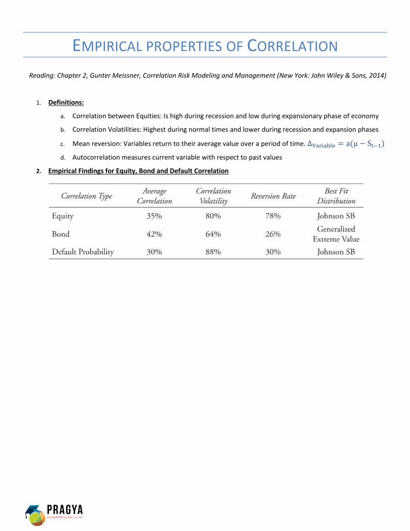
1. Definitions:

a. Correlation between Equities: Is high during recession and low during expansionary phase of economy

b. Correlation Volatilities: Highest during normal times and lower during recession and expansion phases

c. Mean reversion: Variables return to their average value over a period of time. ΔVariable = a(μ − St−1)

d. Autocorrelation measures current variable with respect to past values

2. Empirical Findings for Equity, Bond and Default Correlation

STATISTICAL CORRELATION MODELS

Reading: Chapter 3, Gunter Meissner, Correlation Risk Modeling and Management (New York: John Wiley & Sons, 2014)

1. Limitations of Financial Models:

a. Inaccurate inputs (In times of stress, correlation increase significantly and can't use normal correlations)

b. Erroneous assumptions regarding distributions (BSM assumes constant volatility and not a smile)

c. Mathematical inconsistency (Certain inputs to BSM make models insensitive to implied volatility)

2. Pearson Correlation: Used to measure linear relationships between two variables

a. ρx,y = Covx,y

σxσy where Covx,y =

∑ (xt−μx)(yt−μt)nt=1

n−1

b. The formula ensures that correlation is always between -1 and 1

3. Spearman Rank Correlation: It does not require the knowledge of distribution of the variables

a. ρ = 1 − 6 ∑ di

2ni=1

n(n2−1)

b. Rank all variables in X as 1 to n in order they appear. Then sort all variables from smallest to largest in Y

and rank them 1 to n

c. Calculate difference between ranks and square the difference (this is di2)

4. Kendal τ: Another ordinal measure like Spearman

5. Disadvantages of Ordinal Measures:

a. Only show rank of variables and problems arise when cardinal observations likes quantity or value of

observations are used

FINANCIAL CORRELATION MODELING

Reading: Chapter 4, Gunter Meissner, Correlation Risk Modeling and Management (New York: John Wiley & Sons, 2014)

1. Definitions:

a. Copula: Creates a joint probability distribution between two or more variables

2. Gaussian Copula: Maps distribution of each variable into a Normal distribution

a. Mapping is done on a percentile basis. First, X distribution is mapped to a standard Normal distribution

and then Y distribution is mapped

b. Helps calculate correlation between variables

EMPIRICAL APPROACHES

Reading: Empirical Approaches to Risk Metrics and Hedging (Chapter 6, Bruce Tuckman, Fixed Income Securities, 3rd

Edition (Hoboken, NJ: John Wiley & Sons, 2011))

1. Issues with DV01 Hedging:

a. DV01 hedge assumes that there is no basis risk i.e. yield on bond and hedging instrument rise and fall by

the same amount

2. One variable regression hedge: We plot a regression line with nominal yield as dependent variable and the real

yield as the independent variable. We get an equation of the form Δynominal = α + β Δyreal + ε. From this

equation, we take the value of β and adjust the DV01 hedge as

a. Hedge Value = β x [ DV01Nominal / DV01Real ] x Value of Portfolio

b. Regression hedge assumes that β is constant over time which is not the case

3. PCA (Principal Component Analysis): It provides a single empirical description of term structure behavior, which

can be applied to all bonds. The advantage is that we need to describe the volatility and structure of a small

number of principal components which approximate all movements in term structure.

TERM STRUCTURE MODELS

Reading: The Science of Term Structure Models, (Chapter 7, Bruce Tuckman, Fixed Income Securities, 3rd Edition

(Hoboken, NJ: John Wiley & Sons, 2011))

1. Binomial Rate Model: The model assumes that interest rates can only take one of two possible values in the

next period

a. The values for the interest rate tree should prohibit arbitrage i.e. the current value should be the same

as market value

b.

2. Recombining and Non-recombining: If the interest rate in the middle node is the same irrespective of up or

down move, then the tree is recombining else its non-recombining

3. Constant Maturity Treasury Swap: It is an agreement to swap a floating rate for a treasury rate such as 10-year

rate

a. E.g. 1,000,000 × ሾycmt−Treasuryሿ

2 where ycmt is the semiannual yield of a predetermined maturity at

payment date (Do not forget to add the payoff amount at every node to the discounted value)

4. Black-Scholes-Merton: We cannot use BSM for valuation of Fixed income securities due to assumptions like:

If q = 0.5, then it is called real

world probability. If q ≠ 0, then

the probability is called risk-

neutral (ie. It equates the current

price with market price)

Do not forget to add

a coupon/payoff in

every node value

derived

If current value equals

market observed value, we

call it risk neutral pricing.

a. No upper price bound

b. Risk free rate is constant

c. Bond volatility is constant

5. Fixed Income with Options: Embedded options change the price-yield relationship and hence affect the price

volatility characteristics of the issue

TERM STRUCTURE MODELS

Reading: The Evolution of Short Rates and the Shape of the Term Structure (Chapter 8, Bruce Tuckman, Fixed Income

Securities, 3rd Edition (Hoboken, NJ: John Wiley & Sons, 2011))

1. Expected Rates: If the expected 1 year spot rates for the next three years are r1, r2, r3 then the two year spot

rate is given as ȓ (2) = √(1 + r1)(1 + r2)2 – 1 and 3 year sport rate ȓ (3) = √(1 + r1)(1 + r2)(1 + r3)3

– 1

2. Convexity effect: The difference between the risk neutral spot rate and the middle node rate of the tree is the

convexity effect i.e. when there is uncertainty regarding the future rate, the volatility of expected rates causes

future spot rates to be lower.

3. Jensen’s Inequality: The convexity effect can be measure using a special case of Jensen’s inequality

a. ቂ1

(0.5 ×𝑟1)(0.5 ×𝑟2) ቃ > (0.5

1

(1+𝑟1)) + (0.5

1

(1+𝑟2)) i.e. E ቂ

1

(1+r)ቃ >

1

E[1+r]

b. All else held equal, the value of convexity increases with maturity

4. Risk premium: Risk averse investors will price bonds with a risk premium to compensate them for taking interest

rate risk. This risk premium is added to all interest rates after current spot rate for a year

Risk neutral rate is

9.952% (Derived by

discounting and then

calculating 3 year spot

rate)

TERM STRUCTURE MODELS - DRIFT

Reading: The Art of Term Structure Models: Drift (Chapter 9, Bruce Tuckman, Fixed Income Securities, 3rd Edition

(Hoboken, NJ: John Wiley & Sons, 2011))

1. Model 1(No Drift): It assumes no drift and that interest rates are normally distributed. The continuously

compounded rate rt will change as dr = σ dw where dr is the change in rate over small period of time, dt is

small time interval (measured in years i.e. 1 month will be 1/12), σ is annual basis point volatility of rate change

and dw is normally distributed random variable with mean 0 and standard deviation as ඥdt2

a. Limitations: Volatility is predicted to be flat, only one factor, the short term rate; and any change in

short term rate would lead to a parallel shift in the curve

2. Model 2(Constant Drift): It adds a constant positive drift λdt (positive risk premium) to the model 1 equation,

thus dr = σ dw + λ dt where the drift combines the rate change with a risk premium. The tree is recombining as

in Model 1 but the middle node value dos not equal the first node value

a. Limitations: Calibrated values of drift are often too high, requires forecasting of risk premiums

3. Ho-Lee Model (Time dependent drift): Drift can be negative and is time dependent i.e. drift in time 1 can be

different from drift in time 2. Thus in time 1, dr = σ dw + λ1 dt and in time 2, dr = 2 σ dw + ( λ1 + λ2 )dt

4. Vasicek Model: It assumes a mean reverting process for short term rates. Thus, dr = σ dw + k (θ – r) dt

where k is the speed of mean reversion, θ is the long run value. Also, θ ≈ rLong + λ

k

a. Limitations: Breaks down during period of hyperinflation or similar structural breaks

b. Rate in T years: (θ – r)e−kT and half-life is calculated as (θ – r)e−kT = 1

2 (θ – r)

TERM STRUCTURE –VOLATILITY & DISTRIBUTION

Reading: The Art of Term Structure Models: Volatility and Distribution (Chapter 10, Bruce Tuckman, Fixed Income

Securities, 3rd Edition (Hoboken, NJ: John Wiley & Sons, 2011))

1. Model 3(Time dependent drift and volatility): It augments the Ho-Lee model with time dependent volatility.

Thus, dr = λ(t)+σ e–αt dw where e–αt decreases to 0 exponentially

a. It adds flexibility to models of future short term rates and is useful for pricing multi-period derivatives

like interest rate caps and floors

b. Limitation: Basis point volatility is determined independently of the current short term rate

2. Cox-Ingersoll-Ross (CIR): The annual basis point volatility increases as square root of current short term rate.

Thus, dr = k (θ – r) dt + σ √r2

dw

3. Lognormal Model (Model 4): The volatility of basis points increases with rate. Thus, dr = ar dt + σ r dw where

ar is the drift

a. Deterministic Drift: dr = r0e(a1dt+ σ dw) or dr = r0e[(𝑎1+𝑎2)dt+ 2 σ dw]

b. Mean reversion: r0e[𝑘1(ln 𝜃1−ln 𝑟)dt+ 𝜎1 dw] It is also known as Black-Karasinki model

4. Terminal Distributions of Sort Term Rate after 10 years

OIS DISCOUNTING

Reading: OIS Discounting, Credit Issues, and Funding Costs (Chapter 9, John Hull, Options, Futures, and Other Derivatives,

9th Edition (New York: Pearson, 2014))

1. Definitions:

a. LIBOR: Short term interest rate that creditworthy banks (AA or better) charge each other

b. Federal Funds Rate: rate at which large financial institutions borrow from each other in US

c. OIS (Overnight Indexed Swap): Interest rate swap where fixed(OIS Rate) is exchanged for floating where

floating rate is geometric mean of federal funds rate during the period

2. Disadvantages of Treasury Rates:

a. T-bills and T-Bonds must be purchased by financial institutions and thus increase ind demand drops yield

down

b. Capital required to support investments in T-bills and T-bonds is smaller

c. They get favourable tax treatment in US

3. Disadvantages of LIBOR:

a. LIBOR is volatile in stressed conditions (Spread between LIBOR-OIS during recent financial crisis was 364

basis points)

b. LIBOR incorporates some credit risk. Thus, credit risk may be counted twice

VOLATILITY SMILES

Reading: Reading: Volatility Smiles (Chapter 20, John Hull, Options, Futures, and Other Derivatives, 9th Edition (New

York: Pearson, 2014))

1. Implied Volatility: Implied volatility of a call and put option will be equal for the same strike price and time to

expiration. i.e. PMkt - PBSM = CMkt - CBSM

2. Volatility Smiles: Actual option prices in conjunction with BSM model can be used to derive Implied Volatility.

Implied volatility as a function of strike price generates a volatility smile curve (Options in Currency).

a. Implied volatility is higher for deep in-the-money (ITM)

and out-of-money (OTM) options.

b. This tendency results in greater chance of extreme price

movements than predicted by lognormal distribution

c. Also, long dated options tend to exhibit less of a

volatility smile than shorter dated options.

3. Volatility Skew: The smile is more of a skew for equity options.

a. There is higher implied volatility for low strike price options

(i.e. in-the-money call and out-of-money puts)

b. Probability of large down movements in price is greater than

large up movements

4. Volatility Term Structure: It is a listing of implied volatilities as a function of time to expiration for at-the-money

option contracts

5. Volatility Surface: Combination of volatility smiles with volatility term structure

6. Greeks:

a. Sticky Strike: Implied volatility is the same over short periods of time and greeks are unaffected

b. Sticky Delta: Relationship between options price and ratio of underlying to strike price remains same

7. Price Jumps: Due to price jumps, the volatility smile turns into volatility frown i.e. at-the-money options exhibit

greater implied volatility