Embed Size (px)
Citation preview
1
Machine Learning
Unsupervised Learning
2
Supervised learning vs. unsupervised learning
Supervised learning: discover patterns in the data that relate data attributes with a target (class) attribute. These patterns are then utilized to predict the values
of the target attribute in future data instances Unsupervised learning: The data have no target
attribute. We want to explore the data to find some intrinsic
structures in them.
3
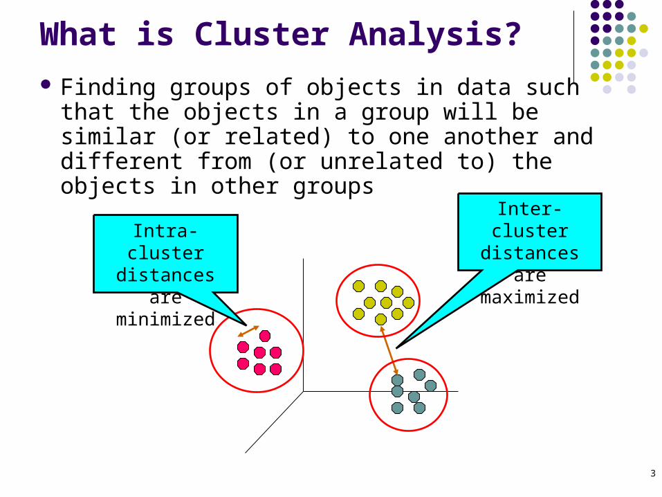
What is Cluster Analysis?
Finding groups of objects in data such that the objects in a group will be similar (or related) to one another and different from (or unrelated to) the objects in other groups
Inter-cluster distances are maximized
Intra-cluster distances are
minimized
4
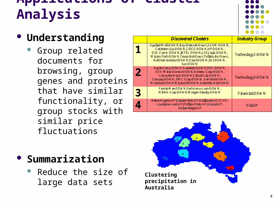
Applications of Cluster Analysis
Understanding Group related documents
for browsing, group genes and proteins that have similar functionality, or group stocks with similar price fluctuations
Summarization Reduce the size of large
data sets
Discovered Clusters Industry Group
1 Applied-Matl-DOWN,Bay-Network-Down,3-COM-DOWN,
Cabletron-Sys-DOWN,CISCO-DOWN,HP-DOWN, DSC-Comm-DOWN,INTEL-DOWN,LSI-Logic-DOWN,
Micron-Tech-DOWN,Texas-Inst-Down,Tellabs-Inc-Down, Natl-Semiconduct-DOWN,Oracl-DOWN,SGI-DOWN,
Sun-DOWN
Technology1-DOWN
2 Apple-Comp-DOWN,Autodesk-DOWN,DEC-DOWN,
ADV-Micro-Device-DOWN,Andrew-Corp-DOWN, Computer-Assoc-DOWN,Circuit-City-DOWN,
Compaq-DOWN, EMC-Corp-DOWN, Gen-Inst-DOWN, Motorola-DOWN,Microsoft-DOWN,Scientific-Atl-DOWN
Technology2-DOWN
3 Fannie-Mae-DOWN,Fed-Home-Loan-DOWN, MBNA-Corp-DOWN,Morgan-Stanley-DOWN
Financial-DOWN
4 Baker-Hughes-UP,Dresser-Inds-UP,Halliburton-HLD-UP,
Louisiana-Land-UP,Phillips-Petro-UP,Unocal-UP, Schlumberger-UP
Oil-UP
Clustering precipitation in Australia

5
Types of Clusterings
A clustering is a set of clusters
Important distinction between hierarchical and partitional sets of clusters
Partitional Clustering A division data objects into non-overlapping subsets
(clusters) such that each data object is in exactly one subset
Hierarchical clustering A set of nested clusters organized as a hierarchical tree

6
Partitional Clustering(Bölümsel Kümeleme)
Original Points A Partitional Clustering
7
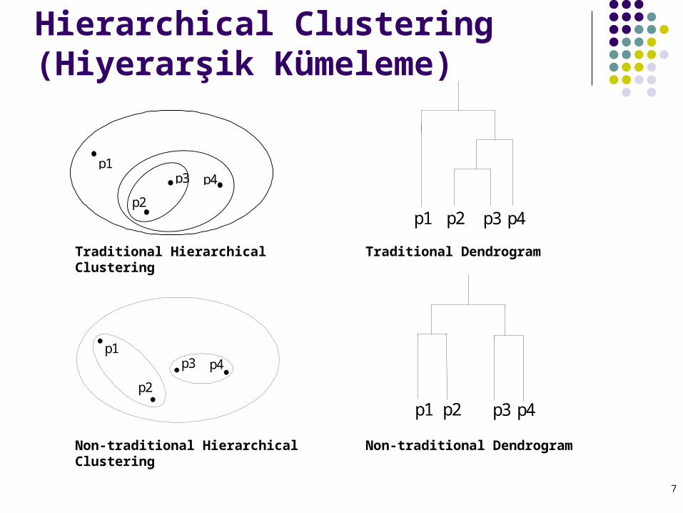
Hierarchical Clustering(Hiyerarşik Kümeleme)
p4p1
p3
p2
p4 p1
p3
p2
p4p1 p2 p3
p4p1 p2 p3
Traditional Hierarchical Clustering
Non-traditional Hierarchical Clustering Non-traditional Dendrogram
Traditional Dendrogram
8
Clustering Algorithms
K-means and its variants
Hierarchical clustering
Density-based clustering
9
K-means clustering
K-means is a partitional clustering algorithm Let the set of data points (or instances) D be
{x1, x2, …, xn}, where xi = (xi1, xi2, …, xir) is a vector in a real-valued space X Rr, and r is the number of attributes (dimensions) in the data.
The k-means algorithm partitions the given data into k clusters. Each cluster has a cluster center, called centroid. k is specified by the user
10
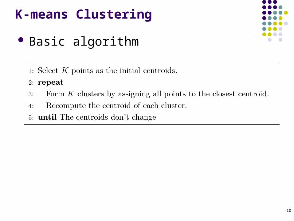
K-means Clustering
Basic algorithm

11
Stopping/convergence criterion
1. no (or minimum) re-assignments of data points to different clusters,
2. no (or minimum) change of centroids, or 3. minimum decrease in the sum of squared error
(SSE),
Ci is the jth cluster, mj is the centroid of cluster Cj (the mean vector of all the data points in Cj), and dist(x, mj) is the distance between data point x and centroid mj.
k
jC jj
distSSE1
2),(x
mx
12
K-means Clustering – Details Initial centroids are often chosen randomly.
Clusters produced vary from one run to another. The centroid is (typically) the mean of the points in the cluster. ‘Closeness’ is measured by Euclidean distance, cosine similarity, correlation, etc. K-means will converge for common similarity measures mentioned above. Most of the convergence happens in the first few iterations.
Often the stopping condition is changed to ‘Until relatively few points change clusters’ Complexity is O( n * K * I * d )
n = number of points, K = number of clusters, I = number of iterations, d = number of attributes
13
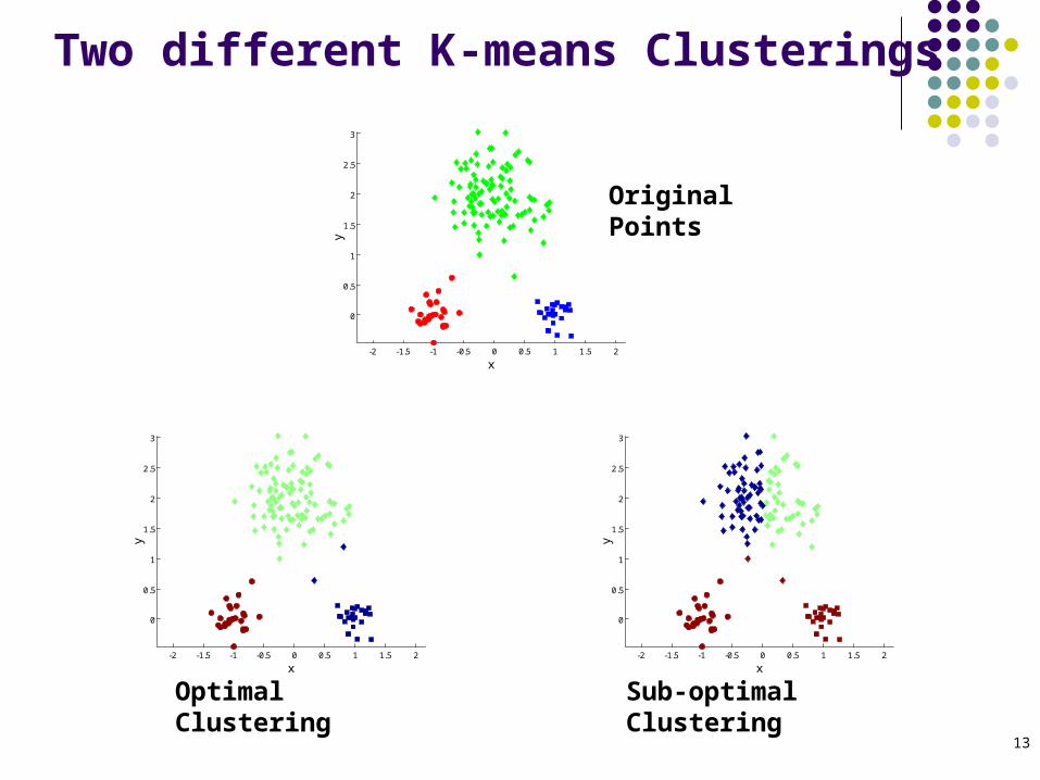
Two different K-means Clusterings
-2 -1.5 -1 -0.5 0 0.5 1 1.5 2
0
0.5
1
1.5
2
2.5
3
x
y
-2 -1.5 -1 -0.5 0 0.5 1 1.5 2
0
0.5
1
1.5
2
2.5
3
x
y
Sub-optimal Clustering
-2 -1.5 -1 -0.5 0 0.5 1 1.5 2
0
0.5
1
1.5
2
2.5
3
x
y
Optimal Clustering
Original Points
14
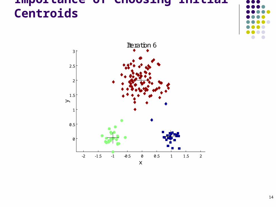
Importance of Choosing Initial Centroids
-2 -1.5 -1 -0.5 0 0.5 1 1.5 2
0
0.5
1
1.5
2
2.5
3
x
y
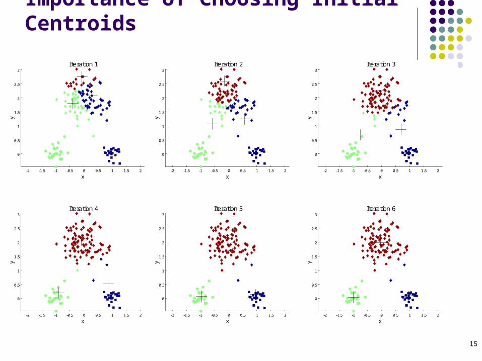
Iteration 1
-2 -1.5 -1 -0.5 0 0.5 1 1.5 2
0
0.5
1
1.5
2
2.5
3
x
y
Iteration 2
-2 -1.5 -1 -0.5 0 0.5 1 1.5 2
0
0.5
1
1.5
2
2.5
3
x
y
Iteration 3
-2 -1.5 -1 -0.5 0 0.5 1 1.5 2
0
0.5
1
1.5
2
2.5
3
x
y
Iteration 4
-2 -1.5 -1 -0.5 0 0.5 1 1.5 2
0
0.5
1
1.5
2
2.5
3
x
y
Iteration 5
-2 -1.5 -1 -0.5 0 0.5 1 1.5 2
0
0.5
1
1.5
2
2.5
3
x
y
Iteration 6
15
Importance of Choosing Initial Centroids
-2 -1.5 -1 -0.5 0 0.5 1 1.5 2
0
0.5
1
1.5
2
2.5
3
x
y
Iteration 1
-2 -1.5 -1 -0.5 0 0.5 1 1.5 2
0
0.5
1
1.5
2
2.5
3
x
y
Iteration 2
-2 -1.5 -1 -0.5 0 0.5 1 1.5 2
0
0.5
1
1.5
2
2.5
3
x
y
Iteration 3
-2 -1.5 -1 -0.5 0 0.5 1 1.5 2
0
0.5
1
1.5
2
2.5
3
x
y
Iteration 4
-2 -1.5 -1 -0.5 0 0.5 1 1.5 2
0
0.5
1
1.5
2
2.5
3
x
y
Iteration 5
-2 -1.5 -1 -0.5 0 0.5 1 1.5 2
0
0.5
1
1.5
2
2.5
3
x
y
Iteration 6
16
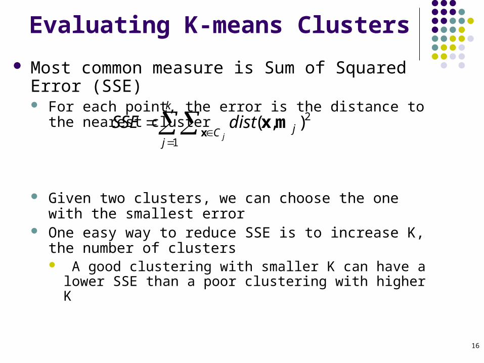
Evaluating K-means Clusters
Most common measure is Sum of Squared Error (SSE) For each point, the error is the distance to the nearest cluster
Given two clusters, we can choose the one with the smallest error
One easy way to reduce SSE is to increase K, the number of clusters A good clustering with smaller K can have a lower SSE than a
poor clustering with higher K
k
jC jj
distSSE1
2),(x
mx
17
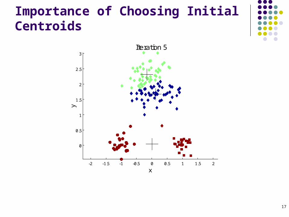
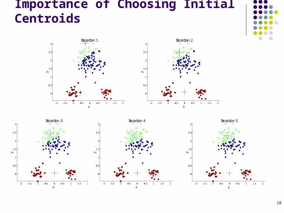
Importance of Choosing Initial Centroids
-2 -1.5 -1 -0.5 0 0.5 1 1.5 2
0
0.5
1
1.5
2
2.5
3
x
y
Iteration 1
-2 -1.5 -1 -0.5 0 0.5 1 1.5 2
0
0.5
1
1.5
2
2.5
3
x
y
Iteration 2
-2 -1.5 -1 -0.5 0 0.5 1 1.5 2
0
0.5
1
1.5
2
2.5
3
x
y
Iteration 3
-2 -1.5 -1 -0.5 0 0.5 1 1.5 2
0
0.5
1
1.5
2
2.5
3
x
y
Iteration 4
-2 -1.5 -1 -0.5 0 0.5 1 1.5 2
0
0.5
1
1.5
2
2.5
3
x
y
Iteration 5
18
Importance of Choosing Initial Centroids
-2 -1.5 -1 -0.5 0 0.5 1 1.5 2
0
0.5
1
1.5
2
2.5
3
x
y
Iteration 1
-2 -1.5 -1 -0.5 0 0.5 1 1.5 2
0
0.5
1
1.5
2
2.5
3
x
y
Iteration 2
-2 -1.5 -1 -0.5 0 0.5 1 1.5 2
0
0.5
1
1.5
2
2.5
3
x
y
Iteration 3
-2 -1.5 -1 -0.5 0 0.5 1 1.5 2
0
0.5
1
1.5
2
2.5
3
x
y
Iteration 4
-2 -1.5 -1 -0.5 0 0.5 1 1.5 2
0
0.5
1
1.5
2
2.5
3
xy
Iteration 5
19
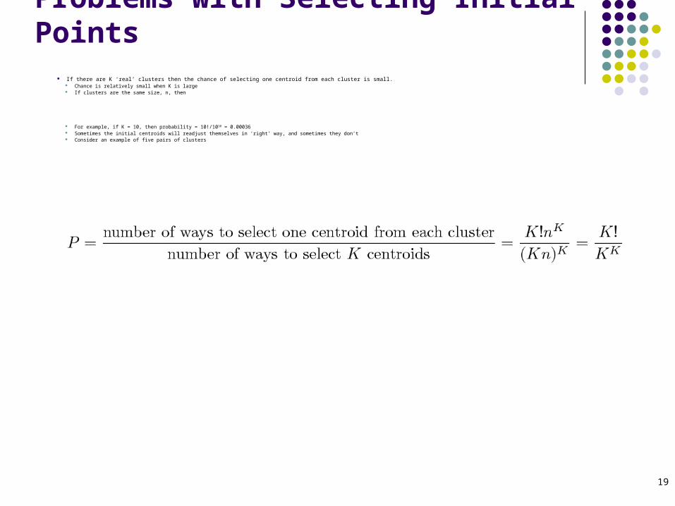
Problems with Selecting Initial Points If there are K ‘real’ clusters then the chance of selecting one centroid from each cluster is small.
Chance is relatively small when K is large If clusters are the same size, n, then
For example, if K = 10, then probability = 10!/1010 = 0.00036 Sometimes the initial centroids will readjust themselves in ‘right’ way, and sometimes they don’t Consider an example of five pairs of clusters

20
10 Clusters Example
0 5 10 15 20
-6
-4
-2
0
2
4
6
8
x
yIteration 1
0 5 10 15 20
-6
-4
-2
0
2
4
6
8
x
yIteration 2
0 5 10 15 20
-6
-4
-2
0
2
4
6
8
x
yIteration 3
0 5 10 15 20
-6
-4
-2
0
2
4
6
8
x
yIteration 4
Starting with two initial centroids in one cluster of each pair of clusters

21
10 Clusters Example
0 5 10 15 20
-6
-4
-2
0
2
4
6
8
x
y
Iteration 1
0 5 10 15 20
-6
-4
-2
0
2
4
6
8
x
y
Iteration 2
0 5 10 15 20
-6
-4
-2
0
2
4
6
8
x
y
Iteration 3
0 5 10 15 20
-6
-4
-2
0
2
4
6
8
x
y
Iteration 4
Starting with two initial centroids in one cluster of each pair of clusters
22
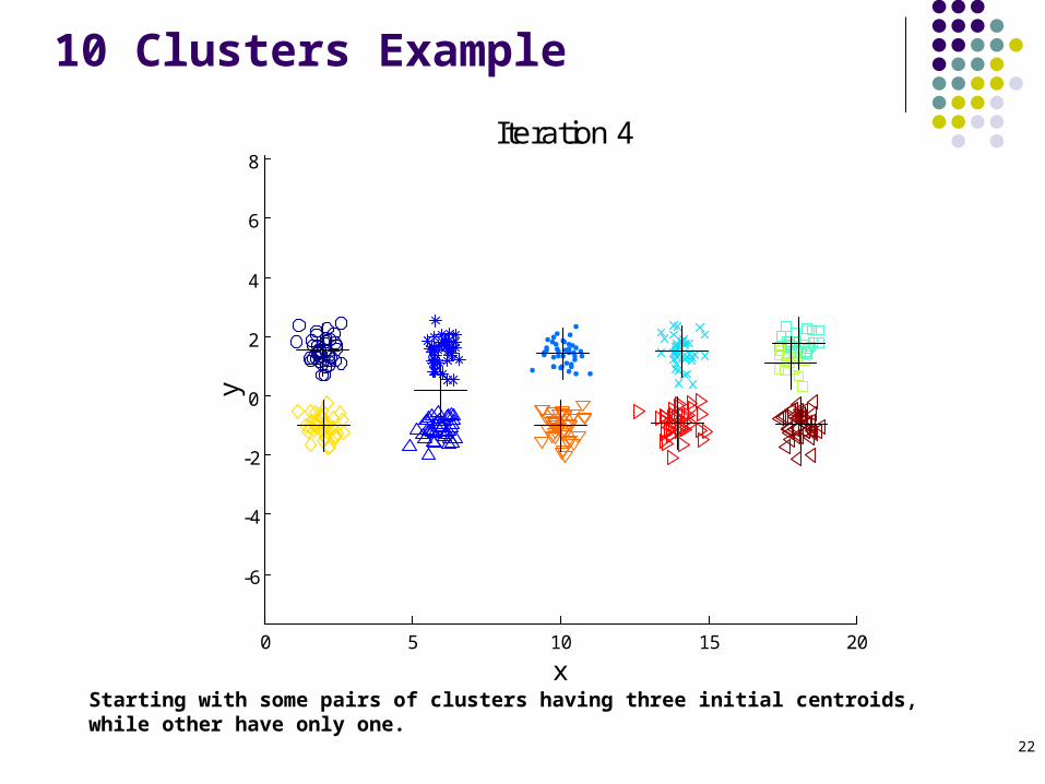
10 Clusters Example
Starting with some pairs of clusters having three initial centroids, while other have only one.
0 5 10 15 20
-6
-4
-2
0
2
4
6
8
x
y
Iteration 1
0 5 10 15 20
-6
-4
-2
0
2
4
6
8
x
y
Iteration 2
0 5 10 15 20
-6
-4
-2
0
2
4
6
8
x
y
Iteration 3
0 5 10 15 20
-6
-4
-2
0
2
4
6
8
x
y
Iteration 4
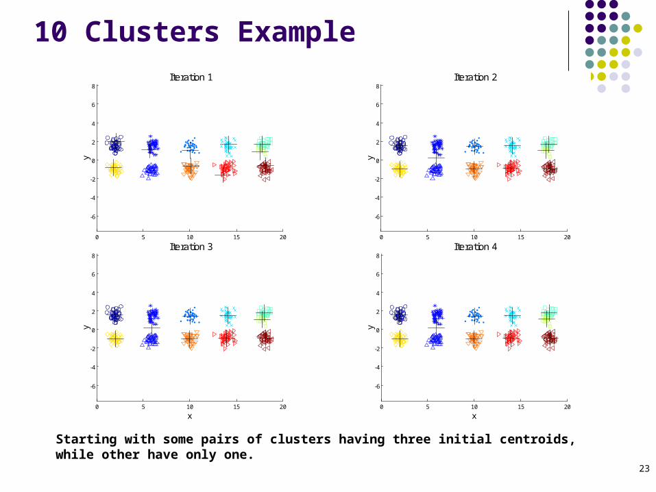
23
10 Clusters Example
Starting with some pairs of clusters having three initial centroids, while other have only one.
0 5 10 15 20
-6
-4
-2
0
2
4
6
8
x
yIteration 1
0 5 10 15 20
-6
-4
-2
0
2
4
6
8
x
y
Iteration 2
0 5 10 15 20
-6
-4
-2
0
2
4
6
8
x
y
Iteration 3
0 5 10 15 20
-6
-4
-2
0
2
4
6
8
x
y
Iteration 4
24
Solutions to Initial Centroids Problem Multiple runs
Helps, but probability is not on your side Sample and use hierarchical clustering to
determine initial centroids Select more than k initial centroids and then
select among these initial centroids Select most widely separated
Postprocessing Bisecting K-means
25
Pre-processing and Post-processing
Pre-processing Normalize the data Eliminate outliers
Post-processing Eliminate small clusters that may represent outliers Split ‘loose’ clusters, i.e., clusters with relatively high SSE Merge clusters that are ‘close’ and that have relatively
low SSE Can use these steps during the clustering process
ISODATA
26
Limitations of K-means
K-means has problems when clusters are of differing Sizes Densities Non-globular shapes
K-means has problems when the data contains outliers.
27
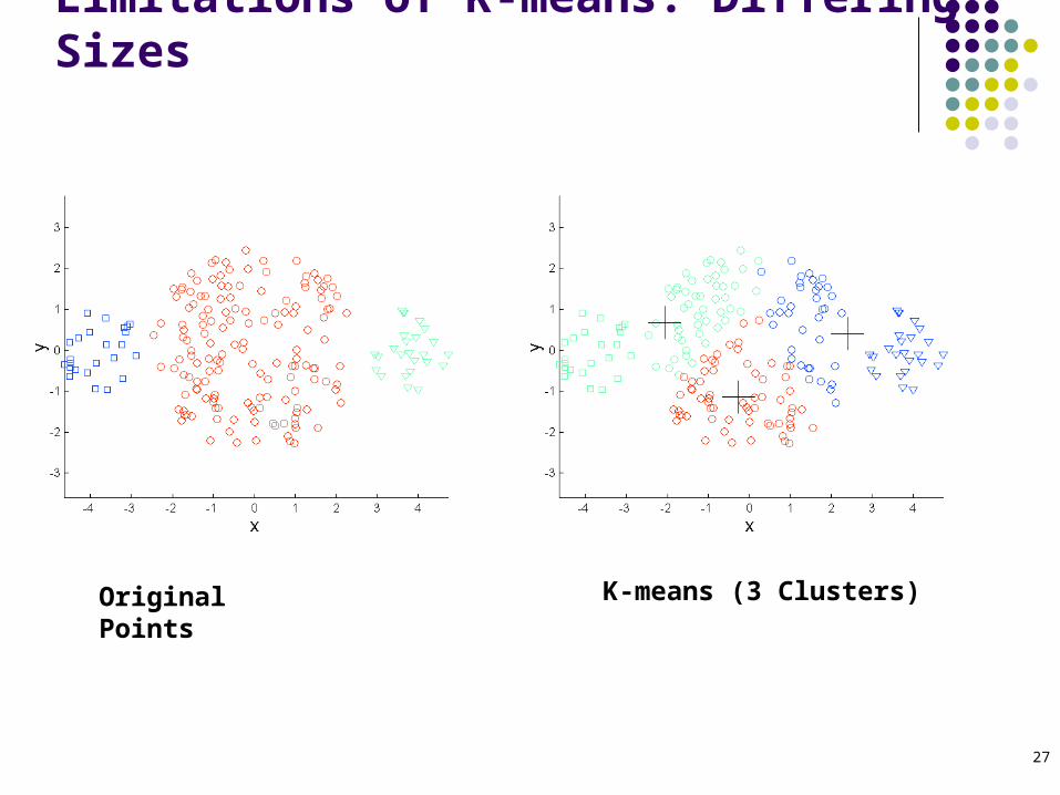
Limitations of K-means: Differing Sizes
Original Points K-means (3 Clusters)
28
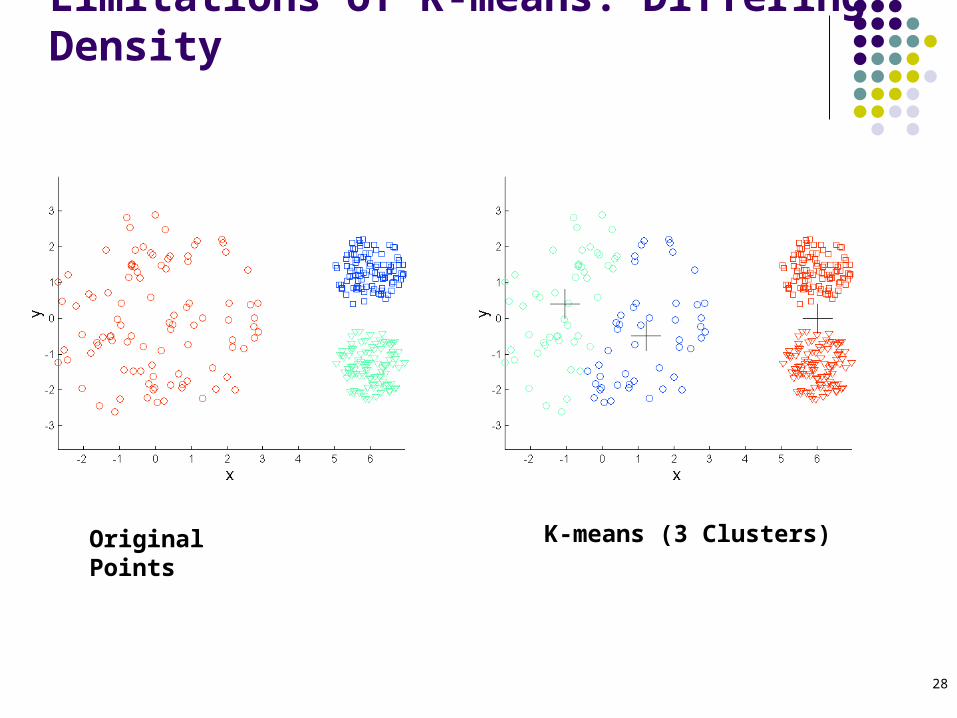
Limitations of K-means: Differing Density
Original Points K-means (3 Clusters)
29
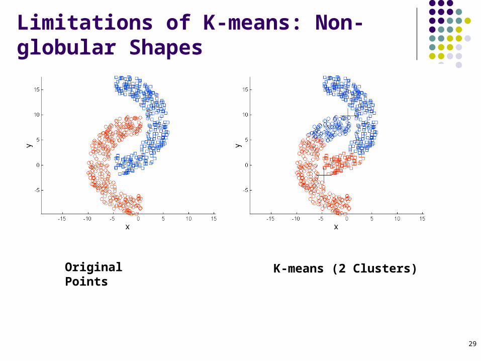
Limitations of K-means: Non-globular Shapes
Original Points K-means (2 Clusters)

30
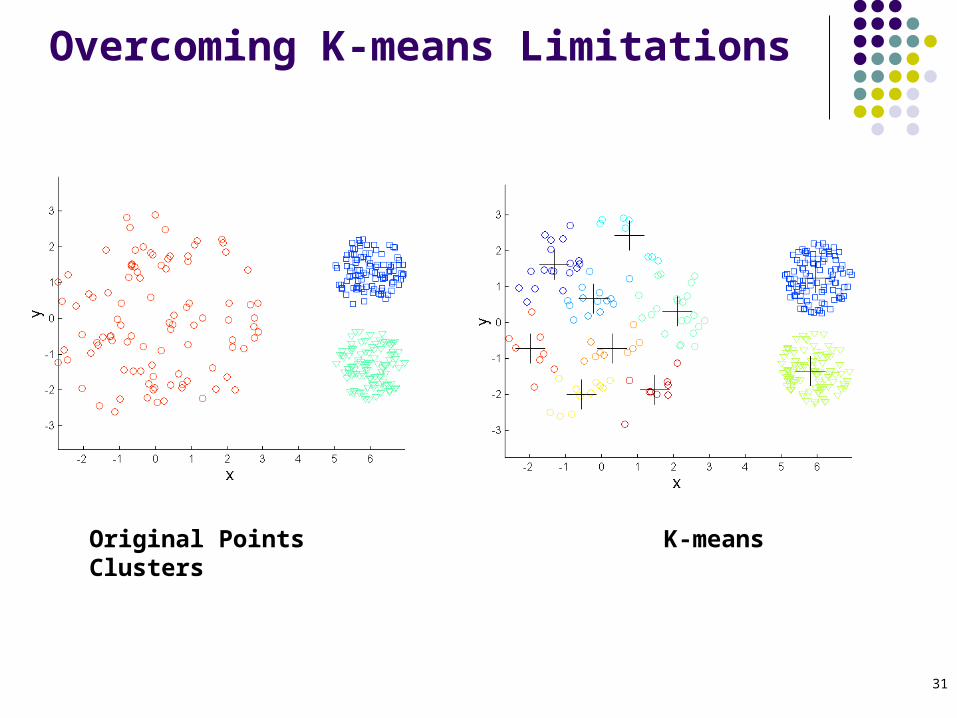
Overcoming K-means Limitations
Original Points K-means Clusters
One solution is to use many clusters.Find parts of clusters, but need to put together.
31
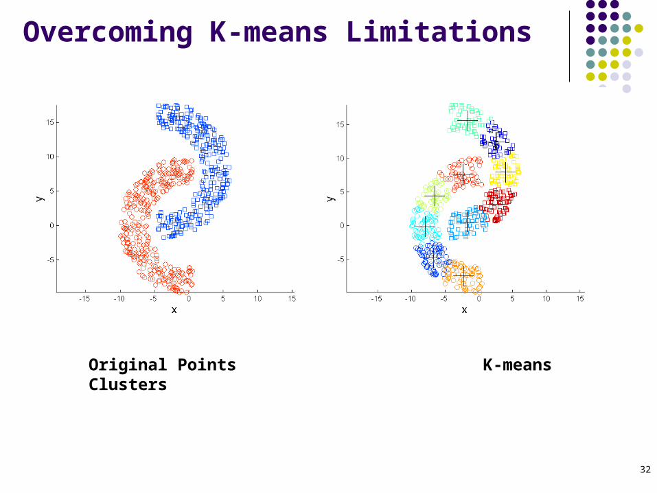
Overcoming K-means Limitations
Original Points K-means Clusters
32
Overcoming K-means Limitations
Original Points K-means Clusters

33
Hierarchical Clustering
Produces a set of nested clusters organized as a hierarchical tree
Can be visualized as a dendrogram A tree like diagram that records the sequences of
merges or splits
1 3 2 5 4 60
0.05
0.1
0.15
0.2
1
2
3
4
5
6
1
23 4
5
34
Strengths of Hierarchical Clustering Do not have to assume any particular number of
clusters Any desired number of clusters can be obtained by
‘cutting’ the dendogram at the proper level
They may correspond to meaningful taxonomies Example in biological sciences (e.g., animal kingdom,
phylogeny reconstruction, …)
35
Hierarchical Clustering
Two main types of hierarchical clustering Agglomerative:
Start with the points as individual clusters At each step, merge the closest pair of clusters until only one cluster (or
k clusters) left
Divisive: Start with one, all-inclusive cluster At each step, split a cluster until each cluster contains a point (or there
are k clusters)
Traditional hierarchical algorithms use a similarity or distance matrix Merge or split one cluster at a time
36
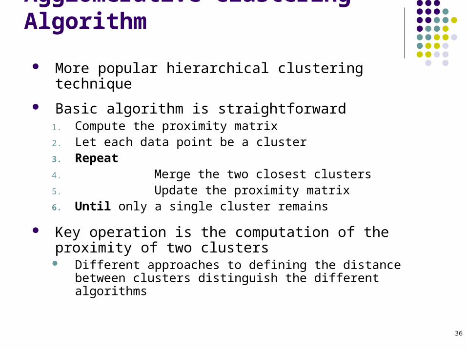
Agglomerative Clustering Algorithm
More popular hierarchical clustering technique Basic algorithm is straightforward
1. Compute the proximity matrix2. Let each data point be a cluster3. Repeat4. Merge the two closest clusters5. Update the proximity matrix6. Until only a single cluster remains
Key operation is the computation of the proximity of two clusters
Different approaches to defining the distance between clusters distinguish the different algorithms

37
Starting Situation
Start with clusters of individual points and a proximity matrix
p1
p3
p5
p4
p2
p1 p2 p3 p4 p5 . . .
.
.
. Proximity Matrix
...p1 p2 p3 p4 p9 p10 p11 p12
38
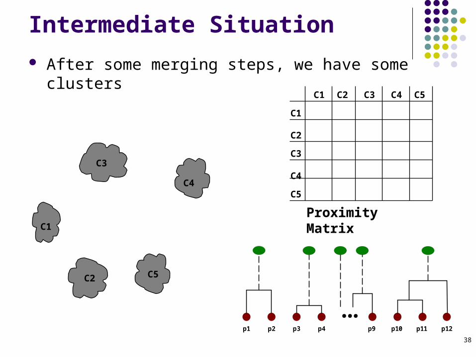
Intermediate Situation
After some merging steps, we have some clusters
C1
C4
C2 C5
C3
C2C1
C1
C3
C5
C4
C2
C3 C4 C5
Proximity Matrix
...p1 p2 p3 p4 p9 p10 p11 p12

39
Intermediate Situation
We want to merge the two closest clusters (C2 and C5) and update the proximity matrix.
C1
C4
C2 C5
C3
C2C1
C1
C3
C5
C4
C2
C3 C4 C5
Proximity Matrix
...p1 p2 p3 p4 p9 p10 p11 p12
40
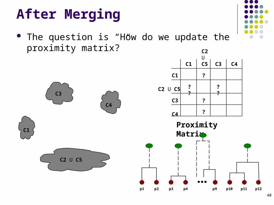
After Merging
The question is “How do we update the proximity matrix?”
C1
C4
C2 U C5
C3? ? ? ?
?
?
?
C2 U C5C1
C1
C3
C4
C2 U C5
C3 C4
Proximity Matrix
...p1 p2 p3 p4 p9 p10 p11 p12

41
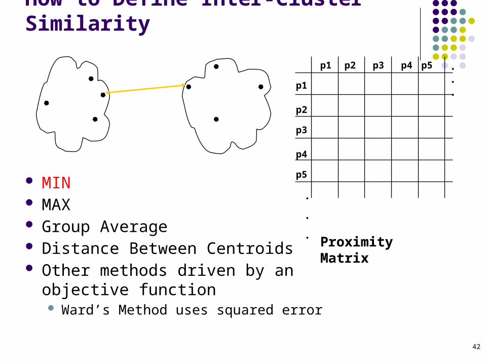
How to Define Inter-Cluster Similarity
p1
p3
p5
p4
p2
p1 p2 p3 p4 p5 . . .
.
.
.
Similarity?
MIN MAX Group Average Distance Between Centroids Other methods driven by an objective
function Ward’s Method uses squared error
Proximity Matrix
42
How to Define Inter-Cluster Similarity
p1
p3
p5
p4
p2
p1 p2 p3 p4 p5 . . .
.
.
.Proximity Matrix
MIN MAX Group Average Distance Between Centroids Other methods driven by an objective
function Ward’s Method uses squared error
43
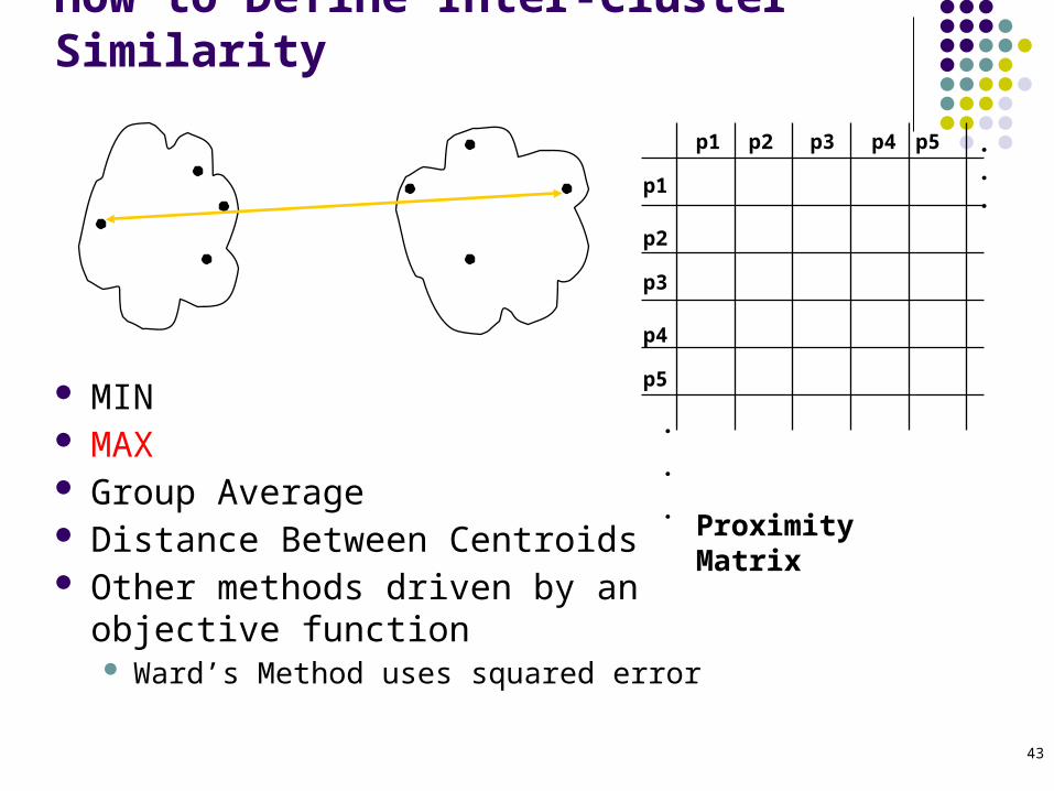
How to Define Inter-Cluster Similarity
p1
p3
p5
p4
p2
p1 p2 p3 p4 p5 . . .
.
.
.Proximity Matrix
MIN MAX Group Average Distance Between Centroids Other methods driven by an objective
function Ward’s Method uses squared error
44
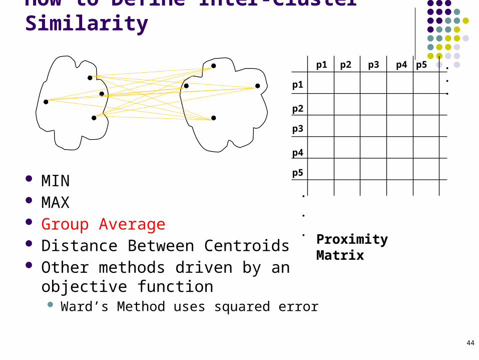
How to Define Inter-Cluster Similarity
p1
p3
p5
p4
p2
p1 p2 p3 p4 p5 . . .
.
.
.Proximity Matrix
MIN MAX Group Average Distance Between Centroids Other methods driven by an objective
function Ward’s Method uses squared error

45
How to Define Inter-Cluster Similarity
p1
p3
p5
p4
p2
p1 p2 p3 p4 p5 . . .
.
.
.Proximity Matrix
MIN MAX Group Average Distance Between Centroids Other methods driven by an objective
function Ward’s Method uses squared error
46
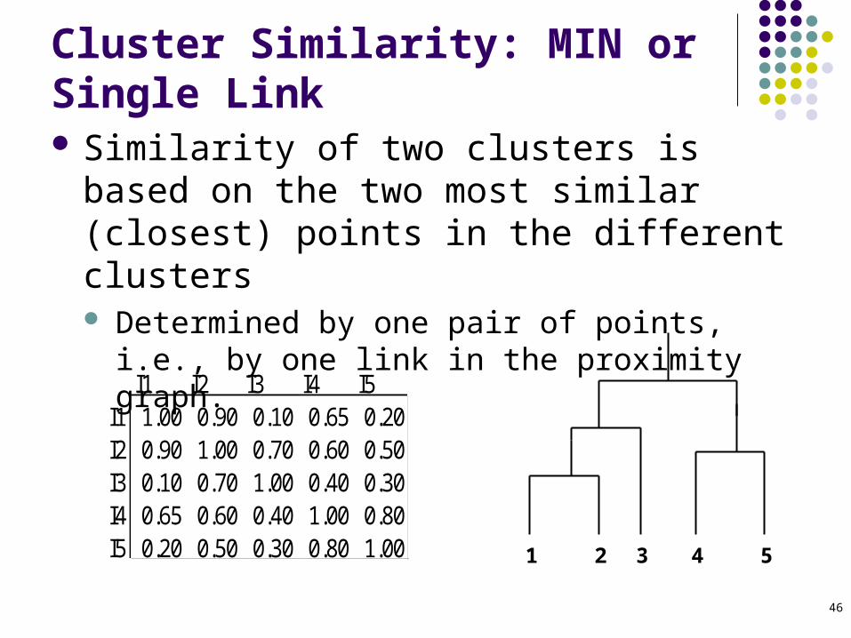
Cluster Similarity: MIN or Single Link Similarity of two clusters is based on the two
most similar (closest) points in the different clusters Determined by one pair of points, i.e., by one link in
the proximity graph.
I1 I2 I3 I4 I5I1 1.00 0.90 0.10 0.65 0.20I2 0.90 1.00 0.70 0.60 0.50I3 0.10 0.70 1.00 0.40 0.30I4 0.65 0.60 0.40 1.00 0.80I5 0.20 0.50 0.30 0.80 1.00 1 2 3 4 5

47
Hierarchical Clustering: MIN
Nested Clusters Dendrogram
1
2
3
4
5
6
1
2
3
4
5
3 6 2 5 4 10
0.05
0.1
0.15
0.2
48
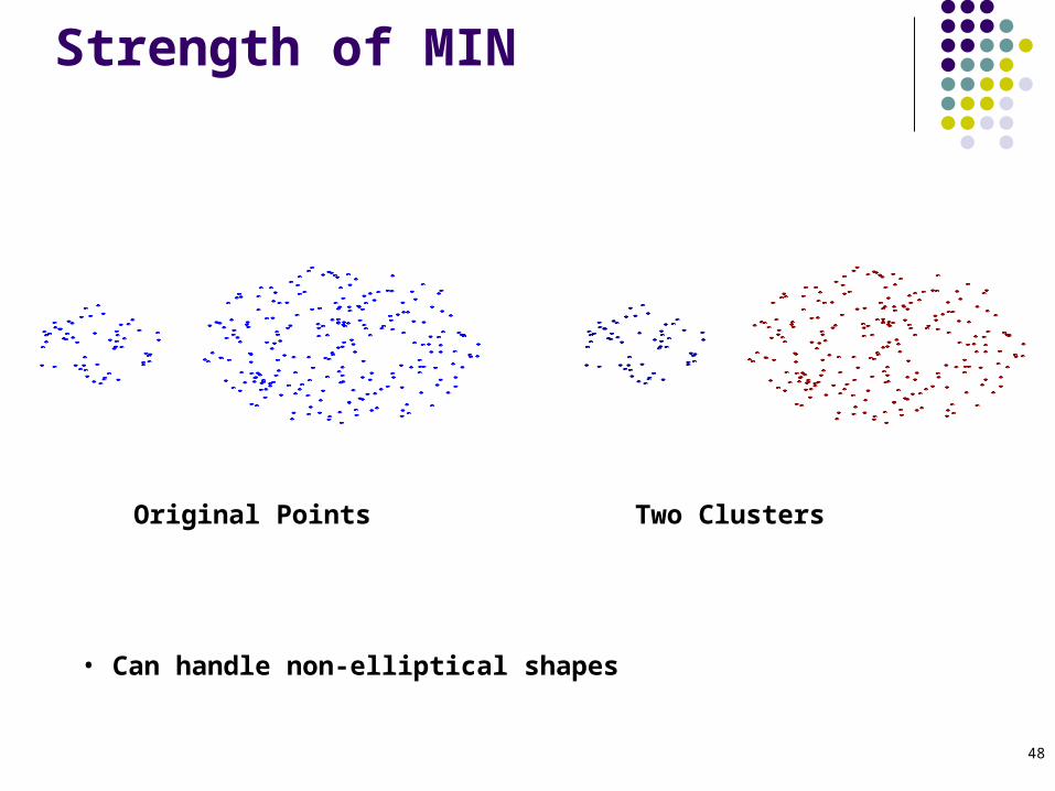
Strength of MIN
Original Points Two Clusters
• Can handle non-elliptical shapes
49
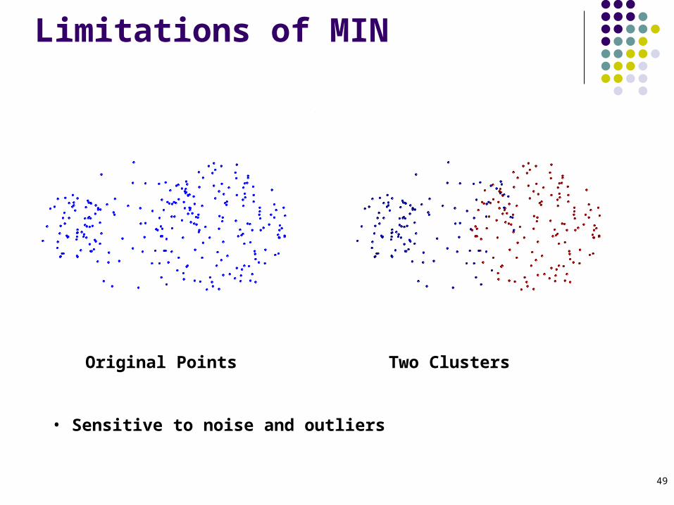
Limitations of MIN
Original Points Two Clusters
• Sensitive to noise and outliers
50
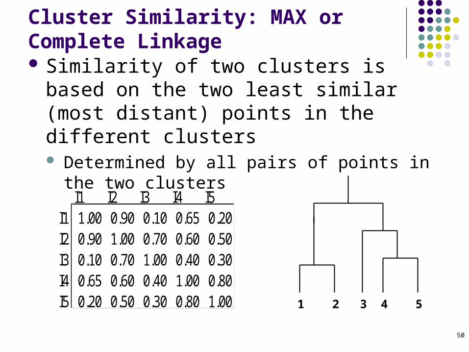
Cluster Similarity: MAX or Complete Linkage Similarity of two clusters is based on the two
least similar (most distant) points in the different clusters Determined by all pairs of points in the two clusters
I1 I2 I3 I4 I5I1 1.00 0.90 0.10 0.65 0.20I2 0.90 1.00 0.70 0.60 0.50I3 0.10 0.70 1.00 0.40 0.30I4 0.65 0.60 0.40 1.00 0.80I5 0.20 0.50 0.30 0.80 1.00 1 2 3 4 5
51
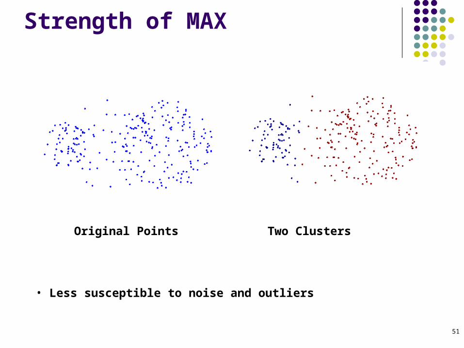
Strength of MAX
Original Points Two Clusters
• Less susceptible to noise and outliers
52
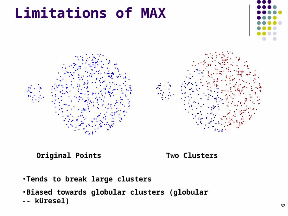
Limitations of MAX
Original Points Two Clusters
•Tends to break large clusters
•Biased towards globular clusters (globular -- küresel)

53
Cluster Similarity: Group Average
Proximity of two clusters is the average of pairwise proximity between points in the two clusters.
Need to use average connectivity for scalability since total proximity favors large clusters
||Cluster||Cluster
)p,pproximity(
)Cluster,Clusterproximity(ji
ClusterpClusterp
ji
jijjii
I1 I2 I3 I4 I5I1 1.00 0.90 0.10 0.65 0.20I2 0.90 1.00 0.70 0.60 0.50I3 0.10 0.70 1.00 0.40 0.30I4 0.65 0.60 0.40 1.00 0.80I5 0.20 0.50 0.30 0.80 1.00 1 2 3 4 5
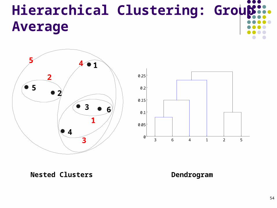
54
Hierarchical Clustering: Group Average
Nested Clusters Dendrogram
3 6 4 1 2 50
0.05
0.1
0.15
0.2
0.25
1
2
3
4
5
6
1
2
5
3
4
55
Hierarchical Clustering: Group Average Compromise between Single and Complete
Link
Strengths Less susceptible to noise and outliers
Limitations Biased towards globular (küresel) clusters
56
Cluster Similarity: Ward’s Method
Similarity of two clusters is based on the increase in squared error when two clusters are merged Similar to group average if distance between points is
distance squared
Less susceptible to noise and outliers
Biased towards globular clusters
Hierarchical analogue of K-means Can be used to initialize K-means
57
Cluster Validity For supervised classification we have a variety of
measures to evaluate how good our model is Accuracy, precision, recall
For cluster analysis, the analogous question is how to evaluate the “goodness” of the resulting clusters?
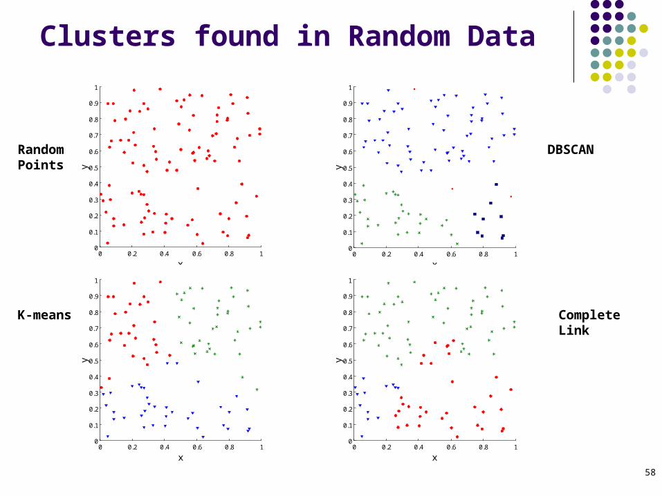
But “clusters are in the eye of the beholder”!
Then why do we want to evaluate them? To avoid finding patterns in noise To compare clustering algorithms To compare two sets of clusters To compare two clusters
58
Clusters found in Random Data
0 0.2 0.4 0.6 0.8 10
0.1
0.2
0.3
0.4
0.5
0.6
0.7
0.8
0.9
1
x
y
Random Points
0 0.2 0.4 0.6 0.8 10
0.1
0.2
0.3
0.4
0.5
0.6
0.7
0.8
0.9
1
x
y
K-means
0 0.2 0.4 0.6 0.8 10
0.1
0.2
0.3
0.4
0.5
0.6
0.7
0.8
0.9
1
x
y
DBSCAN
0 0.2 0.4 0.6 0.8 10
0.1
0.2
0.3
0.4
0.5
0.6
0.7
0.8
0.9
1
x
y
Complete Link
59
1. Determining the clustering tendency of a set of data, i.e., distinguishing whether non-random structure actually exists in the data.
2. Comparing the results of a cluster analysis to externally known results, e.g., to externally given class labels.
3. Evaluating how well the results of a cluster analysis fit the data without reference to external information.
- Use only the data4. Comparing the results of two different sets of cluster analyses to
determine which is better.5. Determining the ‘correct’ number of clusters.
For 2, 3, and 4, we can further distinguish whether we want to evaluate the entire clustering or just individual clusters.
Different Aspects of Cluster Validation
60
Numerical measures that are applied to judge various aspects of cluster validity, are classified into the following three types. External Index: Used to measure the extent to which cluster labels
match externally supplied class labels. Entropy
Internal Index: Used to measure the goodness of a clustering structure without respect to external information.
Sum of Squared Error (SSE) Relative Index: Used to compare two different clusterings or
clusters. Often an external or internal index is used for this function, e.g., SSE or
entropy
Sometimes these are referred to as criteria instead of indices However, sometimes criterion is the general strategy and index is the
numerical measure that implements the criterion.
Measures of Cluster Validity
61
Two matrices Proximity Matrix (Yakınlık matrisi) “Incidence” Matrix (Tekrar Oranı Matrisi)
One row and one column for each data point An entry is 1 if the associated pair of points belong to the same cluster An entry is 0 if the associated pair of points belongs to different clusters
Compute the correlation between the two matrices Since the matrices are symmetric, only the correlation between
n(n-1) / 2 entries needs to be calculated. High correlation indicates that points that belong to the
same cluster are close to each other. Not a good measure for some density or contiguity based
clusters.
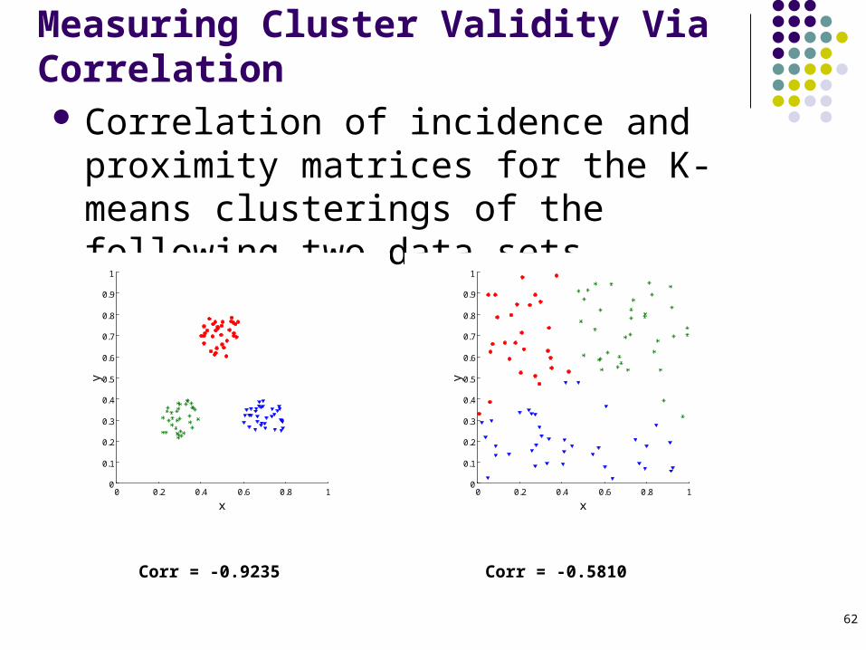
Measuring Cluster Validity Via Correlation
62
Measuring Cluster Validity Via Correlation Correlation of incidence and proximity matrices
for the K-means clusterings of the following two data sets.
0 0.2 0.4 0.6 0.8 10
0.1
0.2
0.3
0.4
0.5
0.6
0.7
0.8
0.9
1
x
y
0 0.2 0.4 0.6 0.8 10
0.1
0.2
0.3
0.4
0.5
0.6
0.7
0.8
0.9
1
x
y
Corr = -0.9235 Corr = -0.5810
63
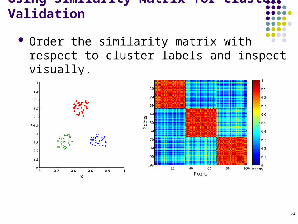
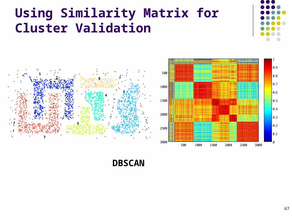
Order the similarity matrix with respect to cluster labels and inspect visually.
Using Similarity Matrix for Cluster Validation
0 0.2 0.4 0.6 0.8 10
0.1
0.2
0.3
0.4
0.5
0.6
0.7
0.8
0.9
1
x
y
Points
Po
ints
20 40 60 80 100
10
20
30
40
50
60
70
80
90
100Similarity
0
0.1
0.2
0.3
0.4
0.5
0.6
0.7
0.8
0.9
1
64
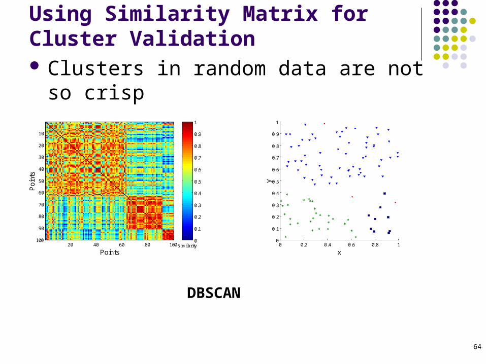
Using Similarity Matrix for Cluster Validation Clusters in random data are not so crisp
Points
Po
ints
20 40 60 80 100
10
20
30
40
50
60
70
80
90
100Similarity
0
0.1
0.2
0.3
0.4
0.5
0.6
0.7
0.8
0.9
1
DBSCAN
0 0.2 0.4 0.6 0.8 10
0.1
0.2
0.3
0.4
0.5
0.6
0.7
0.8
0.9
1
x
y

65
Points
Po
ints
20 40 60 80 100
10
20
30
40
50
60
70
80
90
100Similarity
0
0.1
0.2
0.3
0.4
0.5
0.6
0.7
0.8
0.9
1
Using Similarity Matrix for Cluster Validation Clusters in random data are not so crisp
K-means
0 0.2 0.4 0.6 0.8 10
0.1
0.2
0.3
0.4
0.5
0.6
0.7
0.8
0.9
1
x
y
66
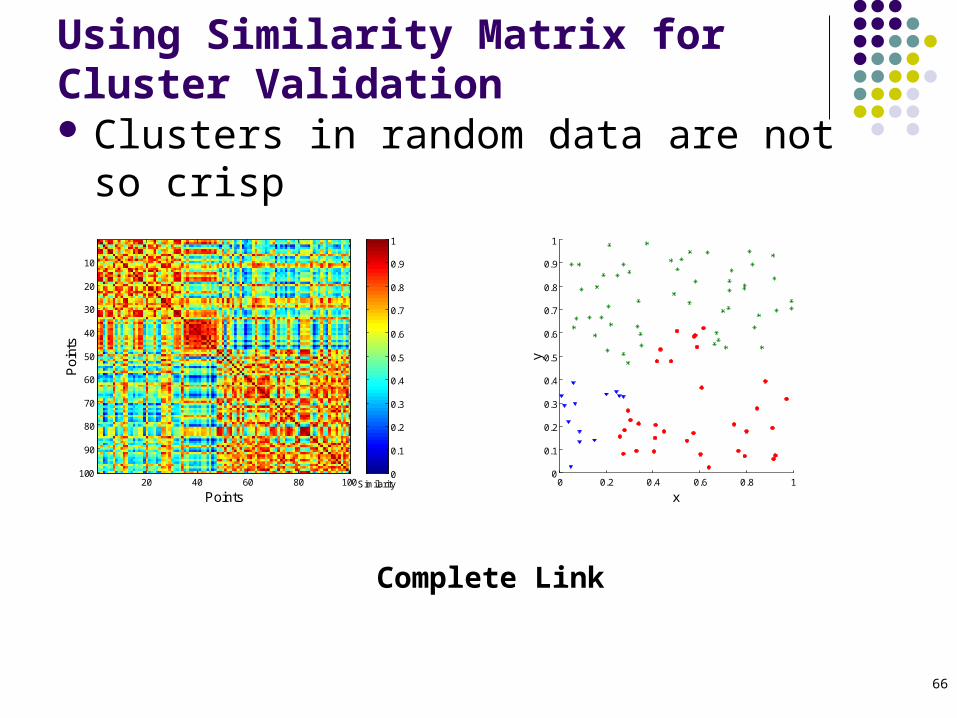
Using Similarity Matrix for Cluster Validation Clusters in random data are not so crisp
0 0.2 0.4 0.6 0.8 10
0.1
0.2
0.3
0.4
0.5
0.6
0.7
0.8
0.9
1
x
y
Points
Po
ints
20 40 60 80 100
10
20
30
40
50
60
70
80
90
100Similarity
0
0.1
0.2
0.3
0.4
0.5
0.6
0.7
0.8
0.9
1
Complete Link
67
Using Similarity Matrix for Cluster Validation
1 2
3
5
6
4
7
DBSCAN
0
0.1
0.2
0.3
0.4
0.5
0.6
0.7
0.8
0.9
1
500 1000 1500 2000 2500 3000
500
1000
1500
2000
2500
3000

68
Cluster Cohesion: Measures how closely related are objects in a cluster Example: SSE
Cluster Separation: Measure how distinct or well-separated a cluster is from other clusters
Example: Squared Error Cohesion is measured by the within cluster sum of squares (SSE)
Separation is measured by the between cluster sum of squares
Where |Ci| is the size of cluster i
Internal Measures: Cohesion and Separation
i Cx
ii
mxWSS 2)(
i
ii mmCBSS 2)(
69
Extra
70
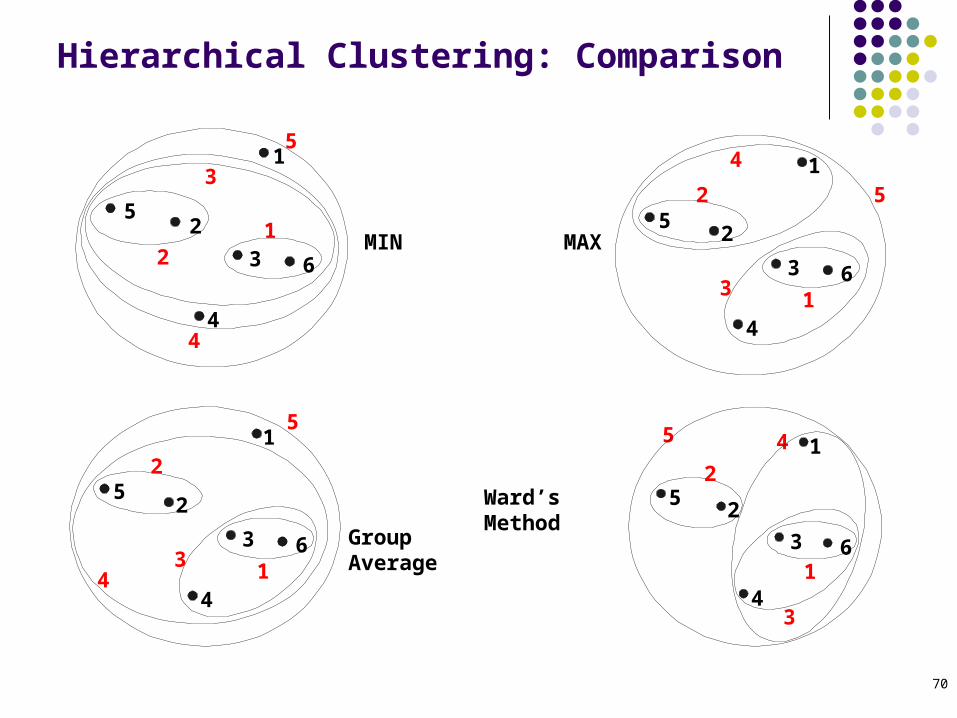
Hierarchical Clustering: Comparison
Group Average
Ward’s Method
1
2
3
4
5
61
2
5
3
4
MIN MAX
1
2
3
4
5
61
2
5
34
1
2
3
4
5
61
2 5
3
41
2
3
4
5
6
12
3
4
5
71
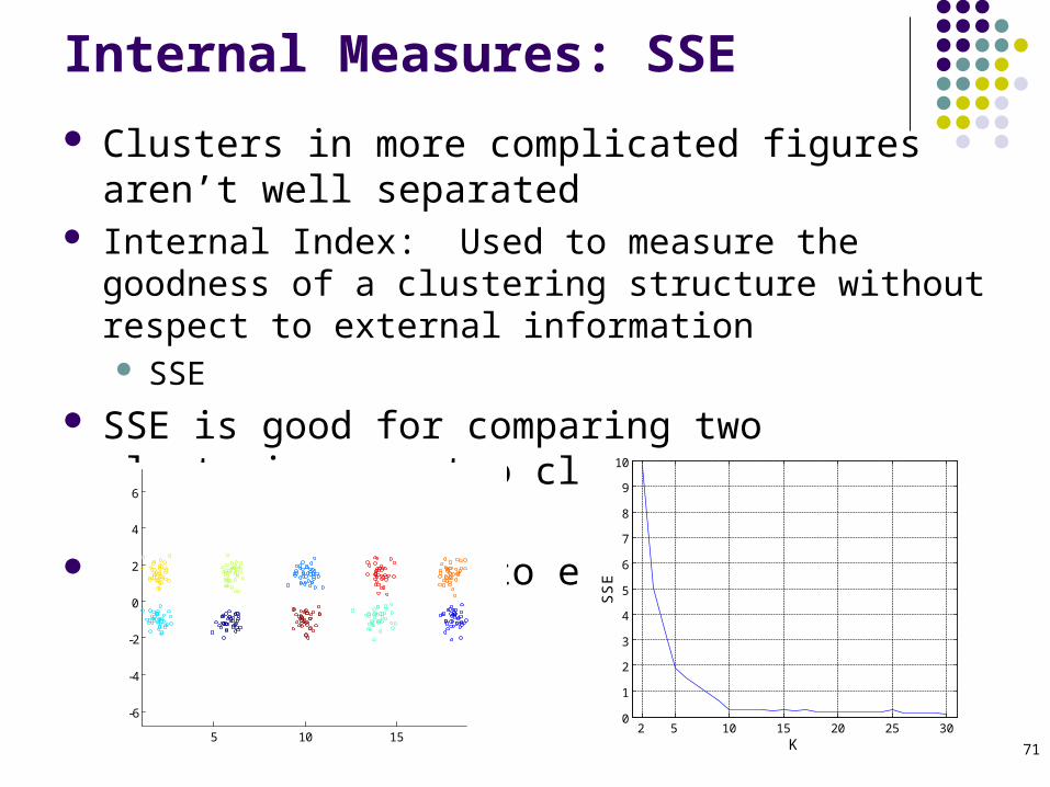
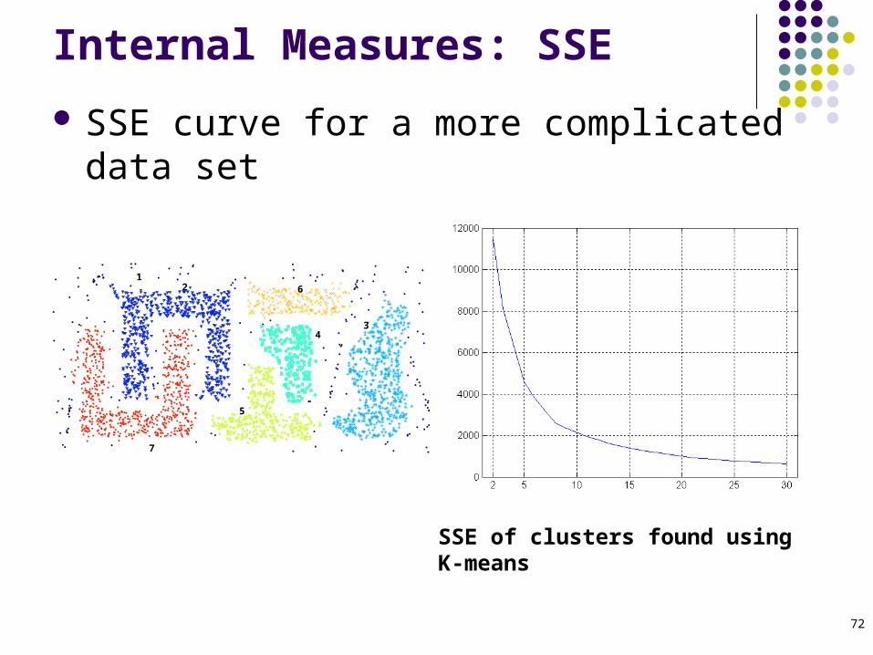
Clusters in more complicated figures aren’t well separated Internal Index: Used to measure the goodness of a clustering
structure without respect to external information SSE
SSE is good for comparing two clusterings or two clusters (average SSE).
Can also be used to estimate the number of clusters
Internal Measures: SSE
2 5 10 15 20 25 300
1
2
3
4
5
6
7
8
9
10
K
SS
E
5 10 15
-6
-4
-2
0
2
4
6
72
Internal Measures: SSE
SSE curve for a more complicated data set
1 2
3
5
6
4
7
SSE of clusters found using K-means

73
Need a framework to interpret any measure. For example, if our measure of evaluation has the value, 10, is that
good, fair, or poor? Statistics provide a framework for cluster validity
The more “atypical” a clustering result is, the more likely it represents valid structure in the data
Can compare the values of an index that result from random data or clusterings to those of a clustering result.
If the value of the index is unlikely, then the cluster results are valid These approaches are more complicated and harder to understand.
For comparing the results of two different sets of cluster analyses, a framework is less necessary.
However, there is the question of whether the difference between two index values is significant
Framework for Cluster Validity

74
Example Compare SSE of 0.005 against three clusters in random data Histogram shows SSE of three clusters in 500 sets of random data
points of size 100 distributed over the range 0.2 – 0.8 for x and y values
Statistical Framework for SSE
0.016 0.018 0.02 0.022 0.024 0.026 0.028 0.03 0.032 0.0340
5
10
15
20
25
30
35
40
45
50
SSE
Co
unt
0 0.2 0.4 0.6 0.8 10
0.1
0.2
0.3
0.4
0.5
0.6
0.7
0.8
0.9
1
x
y
75
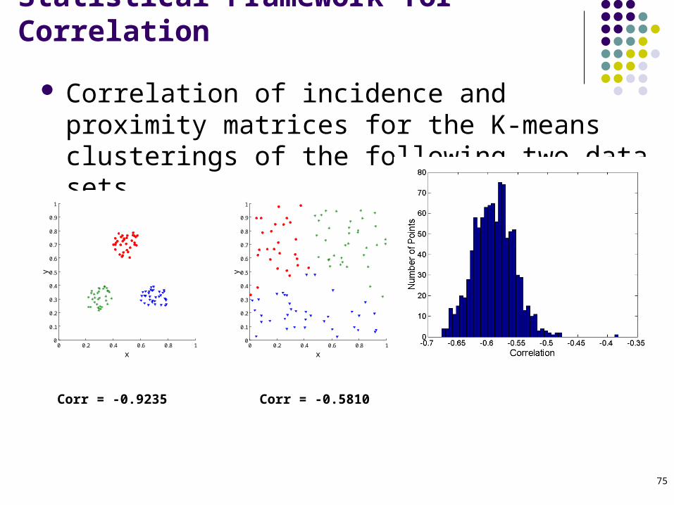
Correlation of incidence and proximity matrices for the K-means clusterings of the following two data sets.
Statistical Framework for Correlation
0 0.2 0.4 0.6 0.8 10
0.1
0.2
0.3
0.4
0.5
0.6
0.7
0.8
0.9
1
x
y
0 0.2 0.4 0.6 0.8 10
0.1
0.2
0.3
0.4
0.5
0.6
0.7
0.8
0.9
1
x
y
Corr = -0.9235 Corr = -0.5810