1 MA421 Introduction

Ashis Gangopadhyay

Department of Mathematics and Statistics

Boston University

c° Ashis Gangopadhyay

1.1 Introduction

1.1.1 Some key statistical concepts

1. • Statistics: Art of data analysis, involving collec-tion, organization and interpretation of data.

• Population: A collection of well defined datathat characterizes some phenomenon.

• Sample: A subset of the population.

• Descriptive statistics: Techniques used to orga-nize and describe sample data.

• Inferential statistics: Techniques used to drawinference about population based on the sampledata.

• Variable: One specific characteristic of the unitsin a give population.

• Observation: A value assigned to the variable.

• Parameter: Descriptive measure of a population.

• Statistic: Descriptive measure of a sample.

• Statistical Inference: Process of making an esti-mate, prediction or decision about a populationbased on sample data.

• Measure of Reliability: A statement about thedegree of uncertainty.

1.1.2 Example: Cola Wars

It is a term that describes intense competition betweenCocaCola and Pepsi. The "war" is fuelled by massiveadvertising campaigns by the two companies, and claimsof consumer preferences for one brand of cola or the other.Suppose a blind taste test, in which the two brand namesare disguised, was conducted to determine the consumerpreference for each of these two brands of cola. Eachof the 1000 participants were asked to state their gender,age, and their preference for either brand A or brand B.

• Population: Collection of all cola consumers.

• Sample: 1000 consumers selected from the popu-lation.

• Variable: Age, Gender, and the preference (A or B)of cola for each individual in the sample.

• Inference of interest: To generalize the consumerpreference of 1000 sampled consumers to the wholepopulation of cola consumers. In particular, we maywant to estimate the percentage of the populationwho prefer Pepsi.

Some more details: Suppose in the sample, 600consumers preferred the taste of Pepsi; i.e., 60% ofthe consumers in the sample preferred Pepsi. Canwe conclude that 60% of the consumers in the pop-ulation also preferred Pepsi? The answer is NO. Itdoes not follow, nor it is likely, that exactly 60% ofthe consumers in the population prefer Pepsi. How-ever, statistical inference techniques tell us that the"true" percentage of the population who prefer Pepsiis almost certainly within a specified limit of the sam-ple estimate.

For example, our analysis may suggest that the sam-ple estimate of the preference for Pepsi is within 3%of the "true" value; implying that the actual prefer-ence for Pepsi in the population is between 57% (=60%-3%) and 63% (= 60% +3%). This intervalrepresents a measure of reliability of the inference.

1.2 Sampling distribution

Population parameter: θ

Sample estimate: bθSuppose we repeatedly draw samples of fixed size fromthe population:

Sample 1 → bθ1Sample 2 → bθ2.....................

Sample k → bθkThe distribution of the collection of estimates {bθ1,cθ2, .., bθk}is called the sampling distribution of bθ.One of the most important result is statistics is the sam-pling distribution of sample mean X as an estimate ofthe population mean µ.

1.2.1 Central Limit Theorem (CLT): Sampling Dis-tribution of X

Suppose n observations are randomly selected from anylarge population with mean µ and standard deviation σ.Then, for n sufficiently large, the sampling distributionof sample mean X is normal with mean µ and standarddeviation (standard error) σ√

n.

Some important observations regarding CLT

• If the population distribution is normal, then the dis-tribution of X is normal for any sample size. How-ever, the distribution of the populations is not nor-mal, then for large sample size (say, for n > 30),

the distribution of X is approximately normal.

• µX = µ

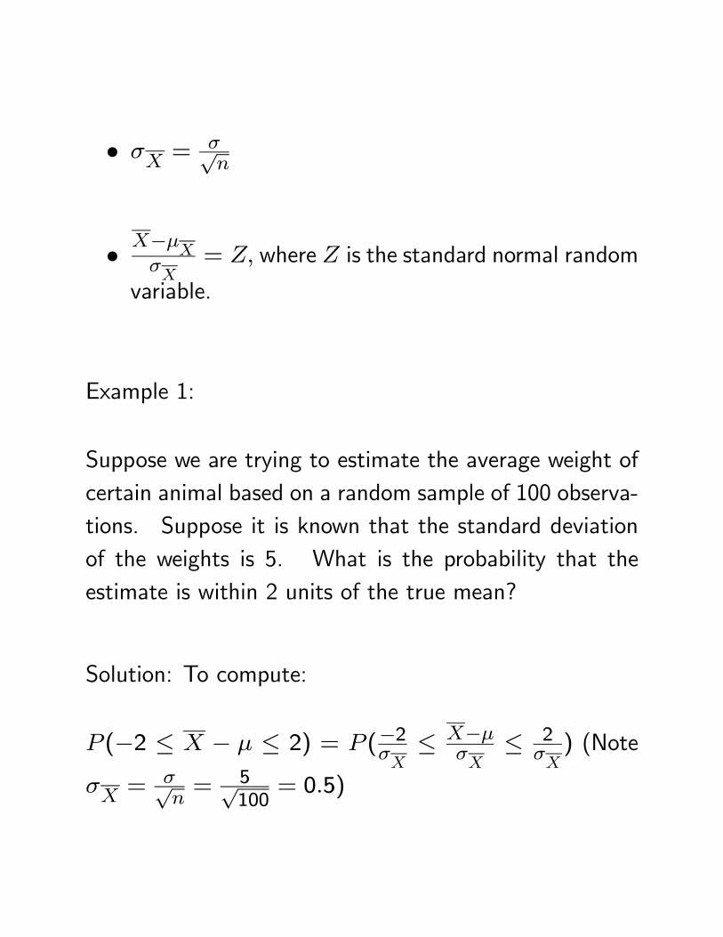
• σX = σ√n

• X−µX

σX

= Z, where Z is the standard normal random

variable.

Example 1:

Suppose we are trying to estimate the average weight ofcertain animal based on a random sample of 100 observa-tions. Suppose it is known that the standard deviationof the weights is 5. What is the probability that theestimate is within 2 units of the true mean?

Solution: To compute:

P (−2 ≤ X − µ ≤ 2) = P (−2σX≤ X−µ

σX≤ 2

σX) (Note

σX = σ√n= 5√

100= 0.5)

= P (−4 ≤ Z ≤ 4)

≈ 1

Thus we are guaranteed to have the sample estimatewithin 2 units of the true mean.

Example 2:

Suppose a bank manager wants to find out the "true" rateat which customers arrive within a 10 minute period atthe branch between 12 - 1 PM. The manager collecteddata between 12 - 1 PM for 30 consecutive days (i.e.,n=180), and found X = 8.1 arrivals per 10 minutes witha standard deviation s = 2.99. Do this data supportmanager’s hypothesis the actual mean arrival rate µ =9?-

Solution: The question is that if the hypothesis is true,and the mean µ = 9, then is it possible to observe asample mean X to be 8.1 or less?

P (X ≤ 8.1) = P (X−µ

XσX

≤ 8.1−90.223 ) = P (Z ≤ −4.04) ≈

0

2 Confidence Interval

A confidence interval estimate provides a range of plau-sible estimates of the parameter of interest.

We use sample information to construct a confidence in-terval, which, with (1−α) ∗ 100% confidence, containsthe true parameter. Thus if an experiment is repeated,and a 95% confidence interval is constructed each time,then we should expect 95% of those intervals to coverthe true value of the parameter.

2.0.2 General form of a confidence interval

Parameter Estimate ± Maximum Error

Note that "±Maximum Error" is also called "Margin ofError."

Maximum Error depends on the sampling distribution ofthe parameter of interest. Suppose we want to estimatea parameter θ, and the sampling distribution of it’s es-timate bθ is normal, then a general form of confidenceinterval is given by:

bθ ± zα2SE(bθ)

In particular: a large sample (n > 30) confidence intervalfor a population mean µ is given by:

X ± zα2

µσ√n

¶

Note that a narrower interval is better than a wider in-terval, as a narrow interval contains more information.

Larger confidence level leads to wider interval.

Larger sample size leads to narrower interval.

Example: Suppose a software company wishes to esti-mate the average number of employees absent per day. Areview of records from the last 100 days revealed that theaverage number of employees absent per day X = 5.1with a standard deviation s = 2.0. Compute 95% confi-dence interval for µ, the true average number of employ-ees absent per day.

Solution: Since 1− α = 0.95, zα2= z0.025 = 1.96

Thus 95% confidence interval is given by:

5.1±1.96( 2√100)

) = (5.1−0.39, 5.1+0.39) = (4.71, 5.49)

Is it possible that the true average number of employeesabsent per day is more than 7?

2.1 Student’s t-distribution

• A continuous distribution that is symmetric aboutzero.

• Characterized by a parameter ν, called degrees offreedom (df). Degrees of freedom ν assumes positiveinteger values.

• A t-distribution with low df has longer tail comparedto standard normal distribution.

• As the df increases, the tails of the t-distributiongets shorter. For ν > 30, there is almost no dif-ference between t-distribution and standard normaldistribution.

http://www.econtools.com/jevons/java/Graphics2D/tDist.html

Fact: If a random sample of size n is selected from anormal population with mean µ, the distribution of thestatistic X−µ

s√nhas a t-distribution with (n − 1) degrees

of freedom.

How do we verify that a population is normally distrib-uted?

• Histogram

• Normal Probability Plot

• Various tests for normality.(more on this topic later)

2.2 Small sample confidence interval for µ

Assuming that the sample observations are from a normalpopulation, a (1 − α) ∗ 100% confidence interval for µis given by

X ± tα2

s√n

Example: Suppose a statistics professor wants to es-timate the average number of classes the undergradu-ate students miss each semester. She randomly selectedten undergraduate students and asked them how manyclasses they missed last semester. The students’ re-sponses are as follows: 4, 7, 2, 0, 1, 0, 10, 2, 0, 3.

Use the data to find 95% confidence interval for µ, theaverage number of classes the students were absent lastsemester.

Solution: NotePX = 29,

PX2 = 183. Thus:

X = 2910 = 2.9

s2 = 1n−1

·PX2 − (

PX)2

n

¸= 19[183− 292

10 ] = 10.98

s =√10.98 = 3.31

Also: (1 − α) = 0.95, tα2= t0.025 = 2.262 based on

df = 9.

95% confidence interval for mean is given by:

2.9± 2.262 ∗µ3.31√10

¶= 2.9± 2.37 = (0.53, 5.27)

2.3 Confidence interval for population pro-

portion p

(1− α) ∗ 100% confidence interval for p is given by

bp± zα2

rbp(1−bp)n

where bp = xn is the sample proportion.

Note: Sample size should be large enough to ensure that

the interval bp±3rbp(1−bp)n does not contain either 0 or 1.

What do we do if the above condition is not met?

Use modified sample proportion ep = x+2n+4, and construct

confidence interval by replacing bp by ep.

Example: Suppose on the election day of the 2004 pres-idential election, 100 randomly selected Massachusettsvoters were asked on their choice of president. 60 of therespondents said that they voted for senator Kerry. Finda 95% confidence interval for the proportion of Massa-chusetts voters who voted for Kerry.

Solution: Is the sample size adequate? bp = 60/100 =0.6

0.6± 3q0.6∗0.4100 = 0.6± 0.15, and the interval does not

include 0 or 1. Thus the sample size is adequate.

95% confidence interval for p is given by:

0.6± 1.96q0.6∗0.4100 = 0.6± 0.096 = (0.504, 0.696)

2.4 Sample size Determination

Sample Size Required to Estimate a Population Mean µwithin E Units of its True Value (i.e., Estimate should bewithin (µ-E, µ+E)).

n =·zα2σ

E

¸2How to find σ?

1. Use a value of σ suggested in previous surveys onthe same variable.

2. If an approximate range, R, on the variable is avail-able, then a crude estimate of is obtained by

σ = R4

Example 1

We want to be 99% sure that a random sample of IQscores yields a mean that is within 2.0 of the true mean.How large should the sample be? Assume that σ is 15.

2.4.1 Sample Size Required to Estimate a Popula-tion Proportion p within E Units of its TrueValue (i.e., Estimate should be within (p-E,p+E))

n =z2α2p(1−p)E2

Note: If prior information about p is available, we canuse that value of p to estimate the sample size. If noinformation is available, use p = 0.5.

Example 2

We want to estimate, with a maximum error of 0.03, thetrue proportion of all TV household turned to a partic-ular show, and we want 95% confidence in our result.How many TV households should be sampled if no priorinformation about p is available?

Example 3

Suppose in the earlier example it is known (from an earliersurvey) that the true proportion p is approximately 0.4.Use this information to recalculate the sample size.