1

Lecture 2Screening and diagnostic tests

• Normal and abnormal

• Validity: “gold” or criterion standard

• Sensitivity, specificity, predictive value

• Likelihood ratio

• ROC curves

• Bias: spectrum, verification, information

2

Clinical/public health applications

• screening: for asymptomatic disease (e.g., Pap test, mammography)

• case-finding: testing of patients for diseases unrelated to their complaint

• diagnostic: to help make diagnosis in symptomatic disease or to follow-up on screening test

3

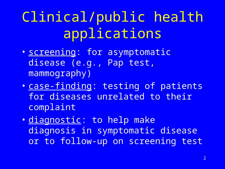
Evaluation of screening and diagnostic tests

• Performance characteristics– test alone

• Effectiveness (on outcomes of disease):– test + intervention

4

Criteria for test selection

• Reproducibility

• Validity

• Feasibility

• Simplicity

• Cost

• Acceptability

5

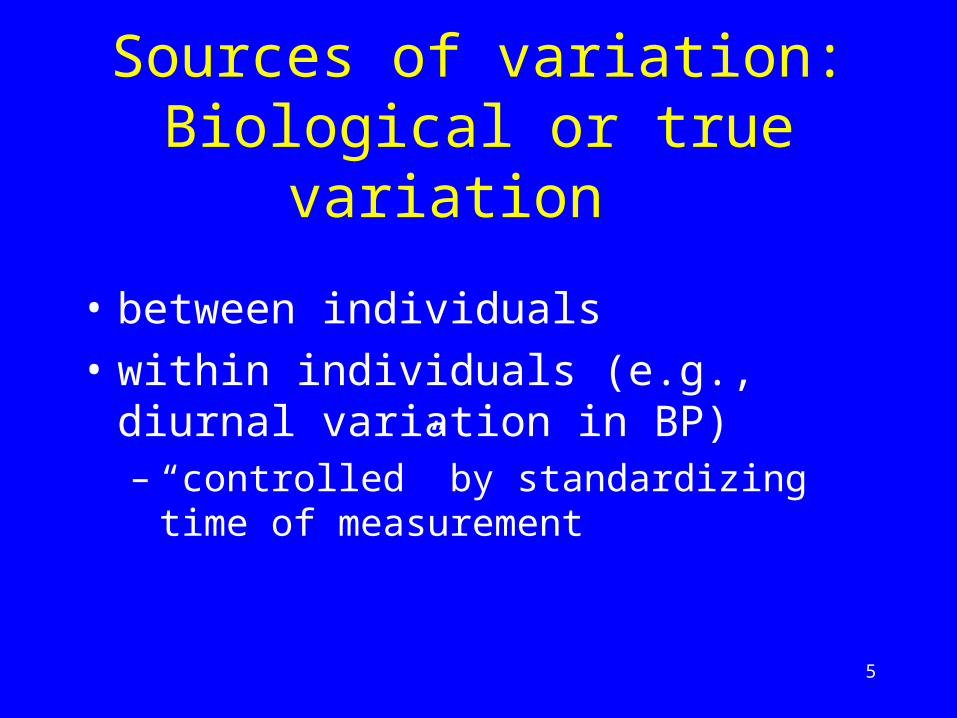
Sources of variation:Biological or true variation

• between individuals

• within individuals (e.g., diurnal variation in BP) – “controlled” by standardizing time of

measurement

6

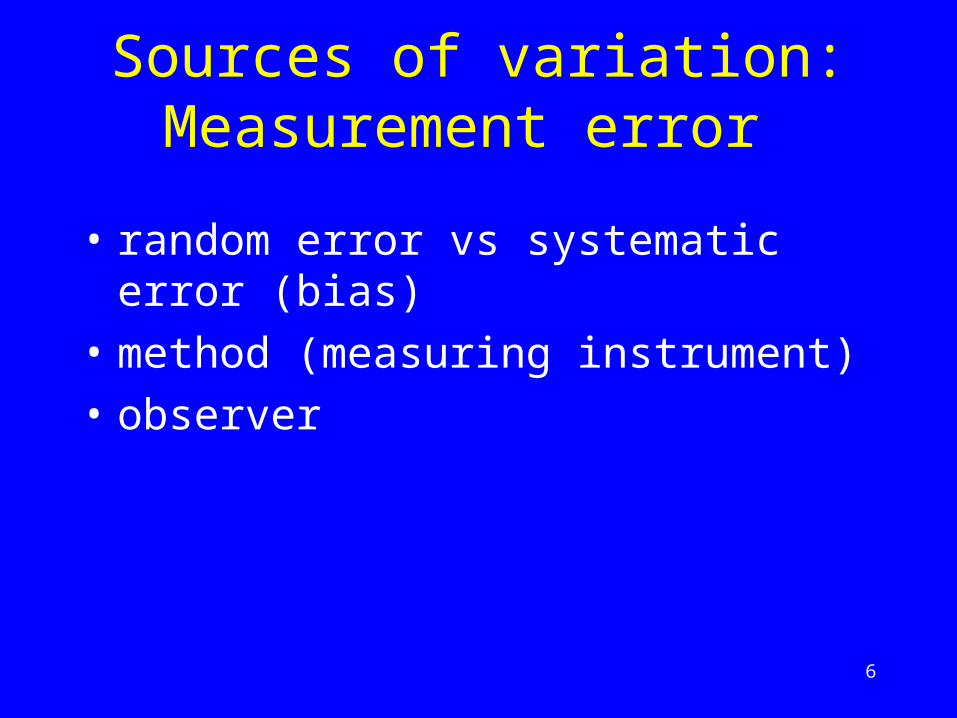
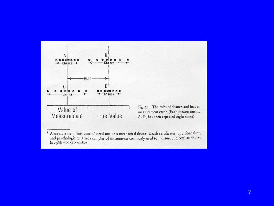
Sources of variation: Measurement error

• random error vs systematic error (bias)

• method (measuring instrument)

• observer

7

8

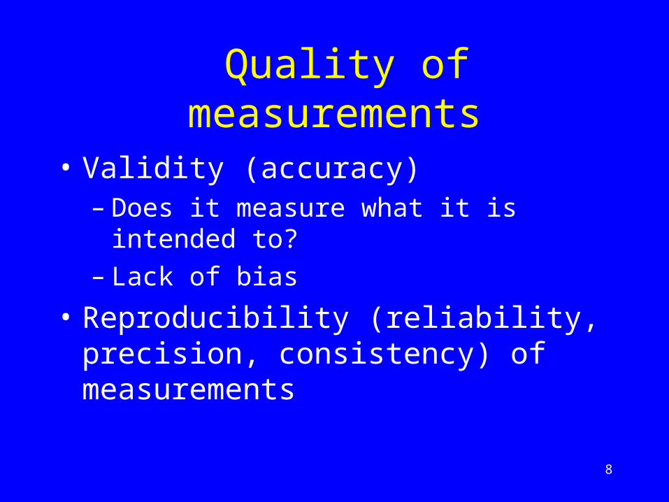
Quality of measurements

• Validity (accuracy) – Does it measure what it is intended to? – Lack of bias

• Reproducibility (reliability, precision, consistency) of measurements

9

Examples of types of reproducibility

• Between and within observer (inter- and intra-observer variation)– May be random or systematic

• Regression toward the mean – Systematic error when subjects have extreme

values (more likely to be in error than typical values)

10

Validity (accuracy)

• Criterion validity – concurrent– predictive

• Face validity, content validity: judgement of the appropriateness of content of measurement

• Construct validity: validity of underlying entity or

theoretical construct

11

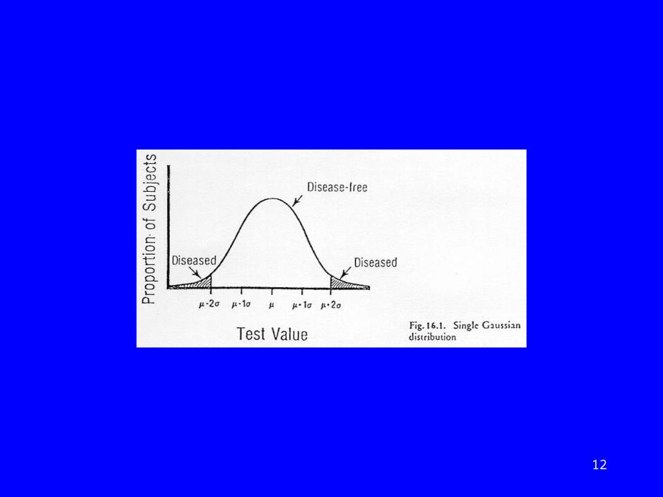
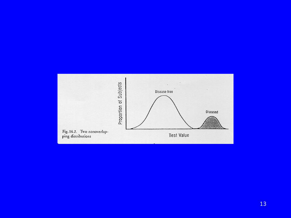
Normal vs abnormal

• Statistical definition– “Gaussian” or “normal” distribution

• Clinical definition – using criterion

12

13

14

15

16

Selection of criterion

• Concurrent– salivary screening test for HIV– history of cough more than 2 weeks (for TB)

• Predictive– APACHE (acute physiology and chronic

disease evaluation) instrument for ICU patients – blood lipid level– maternal height

17

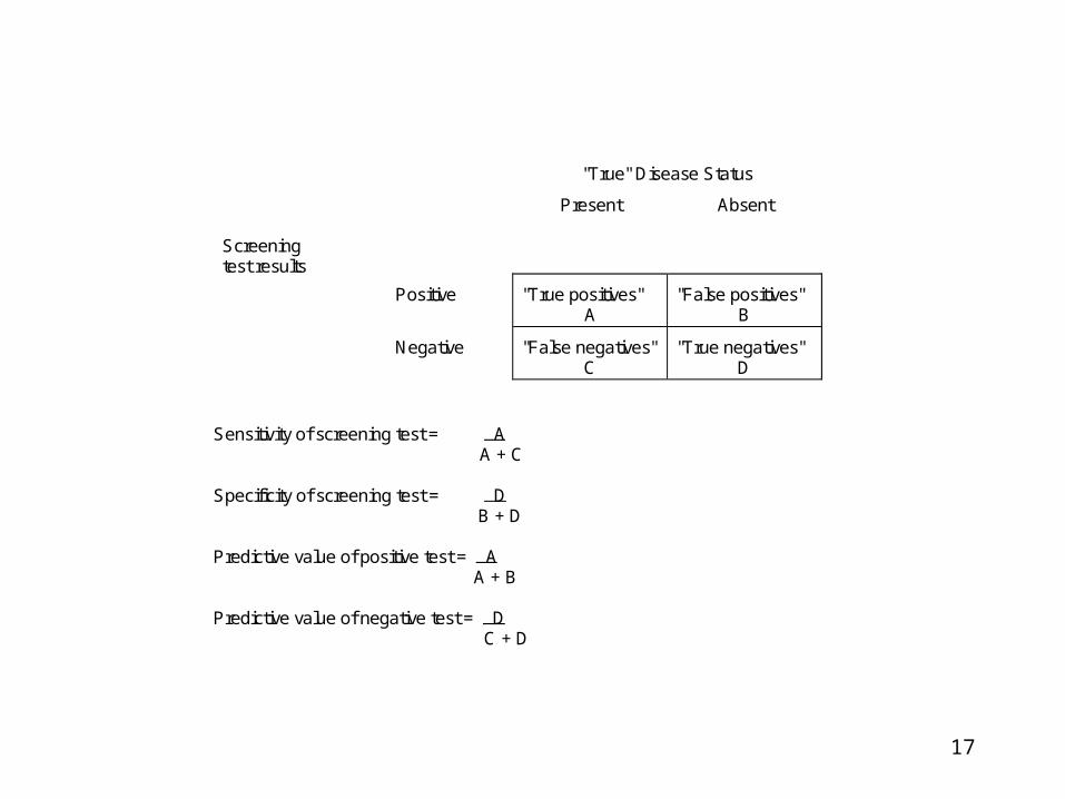
"True" Disease Status

Screeningtest results

Present Absent

Positive "True positives"A

"False positives"B

Negative "False negatives"C

"True negatives"D

Sensitivity of screening test = A A + C

Specificity of screening test = D B + D

Predictive value of positive test = A A + B

Predictive value of negative test = D C + D

18

Sensitivity and specificity

Assess correct classification of:

• People with the disease (sensitivity)

• People without the disease (specificity)

19

Predictive value

• More relevant to clinicians and patients

• Affected by prevalence

20

Choice of cut-point

If higher score increases probability of disease

• Lower cut-point:– increases sensitivity, reduces specificity

• Higher cut-point:– reduces sensitivity, increases specificity

21

Considerations in selection of cut-point

Implications of false positive results

• burden on follow-up services

• labelling effect

Implications of false negative results

• Failure to intervene

22

Likelihood ratio

• Likelihood ratio (LR) = sensitivity

1-specificity

• Used to compute post-test odds of disease from pre-test odds:

post-test odds = pre-test odds x LR

• pre-test odds derived from prevalence

• post-test odds can be converted to predictive value of positive test

23

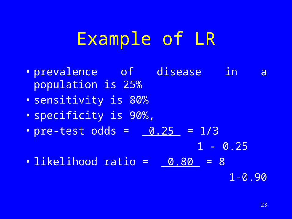
Example of LR

• prevalence of disease in a population is 25%

• sensitivity is 80%

• specificity is 90%,

• pre-test odds = 0.25 = 1/3

1 - 0.25

• likelihood ratio = 0.80 = 8

1-0.90

24

Example of LR

• If prevalence of disease in a population is 25%

• pre-test odds = 0.25 = 1/3

1 - 0.25

• post-test odds = 1/3 x 8 = 8/3

• predictive value of positive result = 8/3+8

= 8/11 = 73%

25

Receiver operating characteristic (ROC) curve

• Evaluates test over range of cut-points

• Plot of sensitivity against 1-specificity

• Area under curve (AUC) summarizes performance:– AUC of 0.5 = no better than chance

26

27

Spectrum bias• Study population should be representative

of population in which test will be used

• Is range of subjects tested adequate?– In population with low risk of outcome,

sensitivity will be lower, specificity higher– In population with high risk of outcome,

sensitivity will be higher, specificity lower

• Comorbidity may affect sensitivity and specificity

28

Verification bias

• results of test affect intensity of subsequent investigation

• increasing probability of detection of outcome in those with positive test result

29

Information bias

• Diagnosis is not blind to test result

• Improves test performance

30

Example: Screening seniors in the emergency department (ED) for risk of

function decline

• High risk group

• Many not adequately evaluated or referred for appropriate services

• Development and validation of a brief screening tool to identify those at increased risk of functional decline and other adverse outcomes

31

Two multi-site studies in Montreal EDs

• Study 1: development of ISAR– Prospective observational cohort study– JAGS (1999) 47: 1226-1237.

• Study 2: evaluation of 2-step intervention – randomized controlled trial– JAGS (2001) 49: 1272-1281.

32

Common features of 2 studies• 4 Montreal hospitals (2 participated in both studies)• Patients aged 65+, community dwelling, English or

French-speaking• Exclusions:

– cognitively impaired or severe illness with no proxy informant

– language barrier (no English or French)

33

Differences between 2 studies: Study design

• Study 1– Observational study– Follow-up at 3 and 6 months after ED visit

• Study 2– Randomized controlled trial: 2-step

intervention vs usual care– Randomization by day of visit– Follow-up at 1 and 4 months after ED visit

34

RESULTS: ISAR development

Adverse health outcome defined as any of following during 6 months after ED visit

• >10% ADL decline

• Death

• Institutionalization

35

Scale development

• Selection of items that predicted all adverse health events

• Multiple logistic regression - “best subsets” analysis

• Review of candidate scales with clinicians to select clinically relevant scale

36

Identification of Seniors At Risk (ISAR)

1. Before the illness or injury that brought you to the Emergency, did you need someone to help you on a regular basis? (yes)

2. Since the illness or injury that brought you to the Emergency, have you needed more help than usual to take care of yourself? (yes)

3. Have you been hospitalized for one or more nights during the past 6 months (excluding a stay in the Emergency Department)? (yes)

4. In general, do you see well? (no)

5. In general, do you have serious problems with your memory? (yes)

6. Do you take more than three different medications every day? (yes)

Scoring: 0 - 6 (positive score shown in parentheses)

37

0

20

40

60

80

0 1 2 3 4 5-6

ISAR SCORE

%

DischargedAdmitted

Any adverse outcome by ISAR score and disposition

38

Other Outcomes Related to ISAR

Source: Dendukuri et al, JAGS, in press

• Does ISAR score identify patients with current functional problems?– Self-reported premorbid function (OARS)– Function at home visit assessed by nurse 1-2

weeks after ED visit (SMAF)

39

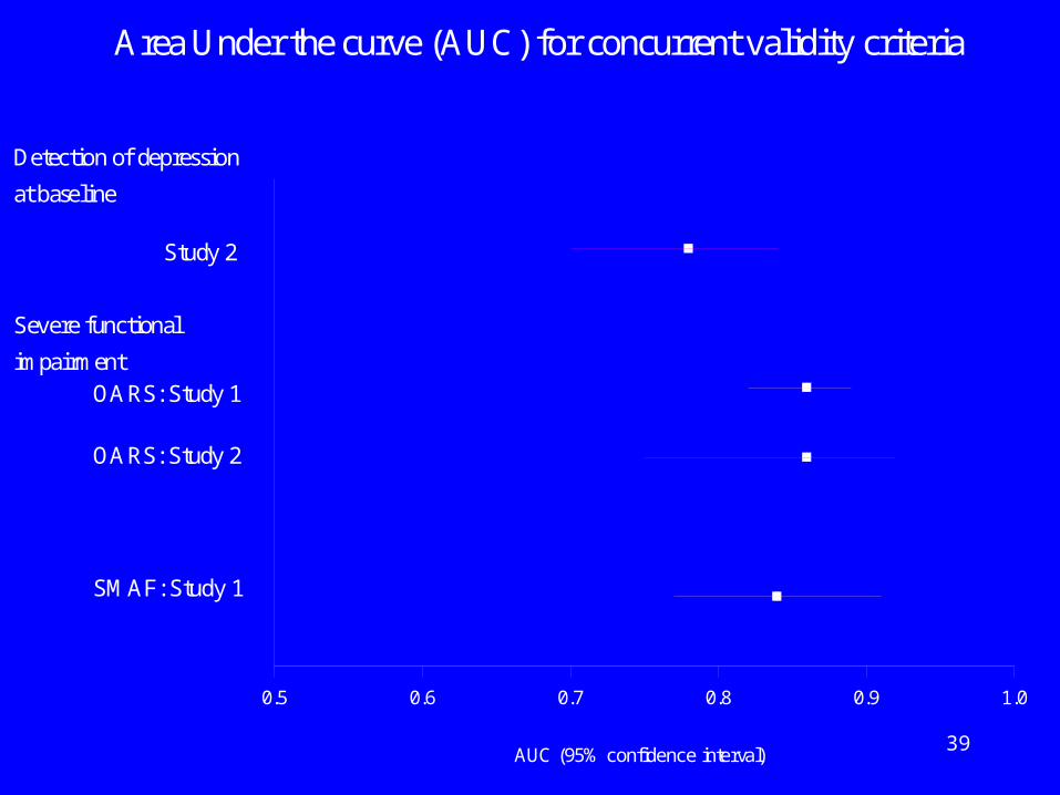
Area Under the curve (AUC) for concurrent validity criteria

Detection of depression

at baseline

Study 2

OARS: Study 1

Severe functional

impairment

OARS: Study 2

SMAF: Study 1

AUC (95% confidence interval)

0.5 0.6 0.7 0.8 0.9 1.0

40

Other Outcomes Related to ISAR

• Does ISAR predict adverse outcomes (other than functional decline) during the subsequent 5 or 6 months?– High hospital utilization (11+ days/5 months)– Frequent ED visits– Frequent community health center visits– Increase in depressive symptoms

41

Area Under the Curve(AUC) for predictive validation criteriaamong patients discharged from ED

Increase in depressivesymptoms

Study 2

10+ community healthcenter visits/5 months

Study 2

11+ hospital days/ 5 months

Study 1

Study 2

2+ ED visits/ 5 months

Study 1

Study 2

Adverse health outcome

Study 1

AUC (95% confidence interval)

0.5 0.6 0.7 0.8 0.9 1.0

42

Summary of data on performance

• Very good detection of patients with current functional problems and depression (AUC values 0.8 - 0.9)

• Moderate ability to predict future adverse health events (functional decline) and health center utilization (AUC values around 0.7)

• Fair ability to predict future hospital and ED utilization (AUC values 0.6 - 0.7)

43

Comparison with other screening tools for patients admitted to hospital

Source: McCusker et al, J Gerontol 2002; 57A: M569-577

• Systematic literature review

• Predictors of functional decline (including nursing home admission) among hospitalized seniors

• Investigated individual risk factors and predictive indices

44

Predictive indices

• Inouye (1993): FD and NH at 3 mo– 4 factors: decubitus ulcer, cognitive

impairment, premorbid functional impairment, low social activity

• Mateev(1998): D/NH at 3 mo. – clinical targeting criteria

45

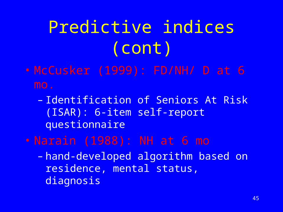
Predictive indices (cont)

• McCusker (1999): FD/NH/ D at 6 mo.– Identification of Seniors At Risk (ISAR): 6-

item self-report questionnaire

• Narain (1988): NH at 6 mo– hand-developed algorithm based on residence,

mental status, diagnosis

46

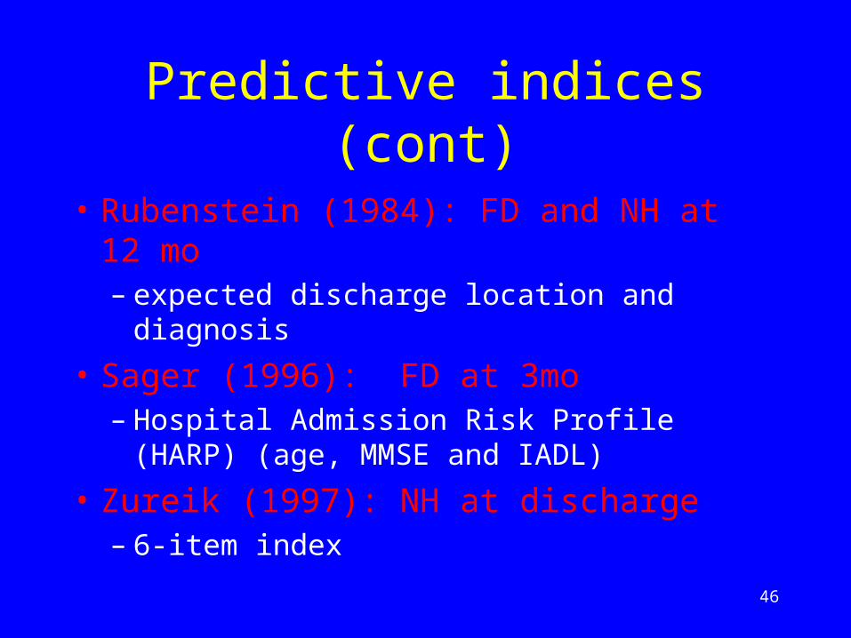
Predictive indices (cont)

• Rubenstein (1984): FD and NH at 12 mo – expected discharge location and diagnosis

• Sager (1996): FD at 3mo– Hospital Admission Risk Profile (HARP) (age,

MMSE and IADL)

• Zureik (1997): NH at discharge– 6-item index

47

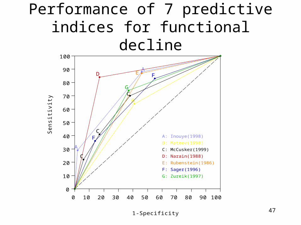
Performance of 7 predictive indices for functional decline

1-Specificity

Se

nsitiv

ity

C

C

C

A

A

B

D E

F

F

G

0

10

20

30

40

50

60

70

80

90

100

0 10 20 30 40 50 60 70 80 90 100

A: Inouye(1998)

B: Mateev(1998)

C: McCusker(1999)

D: Narain(1988)

E: Rubenstein(1986)

F: Sager(1996)

G: Zureik(1997)

48

Performance of predictive indices

• Moderate performance (AUC 0.65 - 0.66)