1

Lecture 2 - Flow Fields

Applied Computational Fluid Dynamics

Instructor: André Bakker

© André Bakker (2002-2004)© Fluent Inc. (2002)

2

Important variables

• Pressure and fluid velocities are always calculated in conjunction. Pressure can be used to calculate forces on objects, e.g. for the prediction of drag of a car. Fluid velocities can be visualized to show flow structures.

• From the flow field we can derive other variables such as shear and vorticity. Shear stresses may relate to erosion of solid surfaces. Deformation of fluid elements is important in mixing processes. Vorticity describes the rotation of fluid elements.

• In turbulent flows, turbulent kinetic energy and dissipation rate are important for such processes as heat transfer and mass transfer in boundary layers.

• For non-isothermal flows, the temperature field is important. This may govern evaporation, combustion, and other processes.

• In some processes, radiation is important.

3

Post-processing

• Results are usually reviewed in one of two ways. Graphically or alphanumerically.

• Graphically:– Vector plots.– Contours. – Iso-surfaces.– Flowlines.– Animation.

• Alphanumerics:– Integral values.– Drag, lift, torque calculations.– Averages, standard deviations.– Minima, maxima.– Compare with experimental data.

4

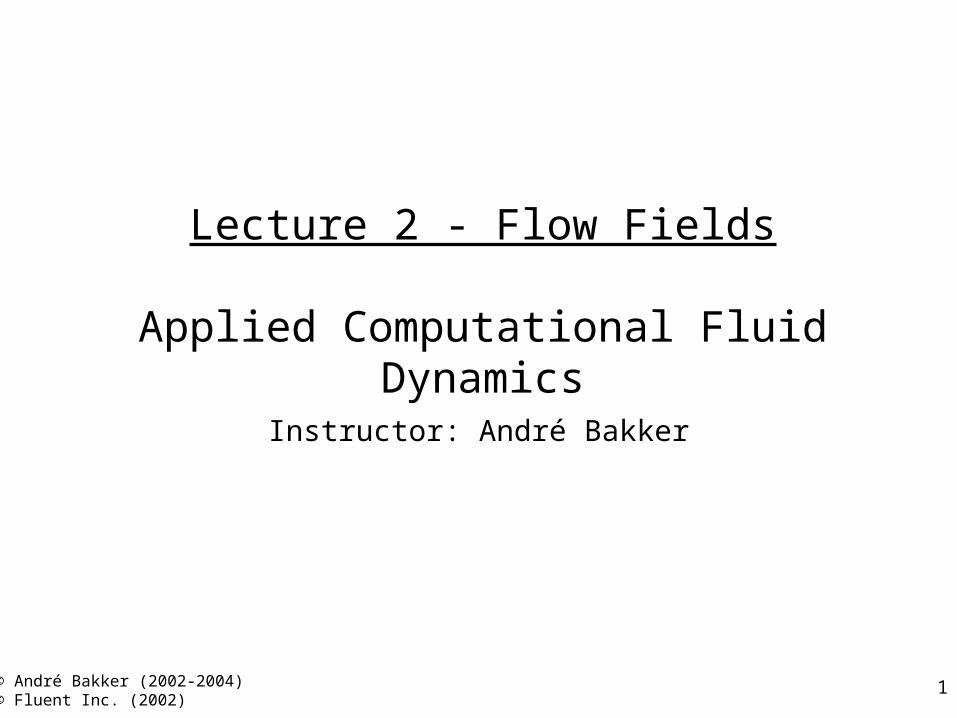
A flow field example: the football

• Regulation size american football.

• Perfect throw. Ball is thrown from right to left.

• Flow field relative to the ball is from left to right.

• Shown here are filled contours of velocity magnitude.

5

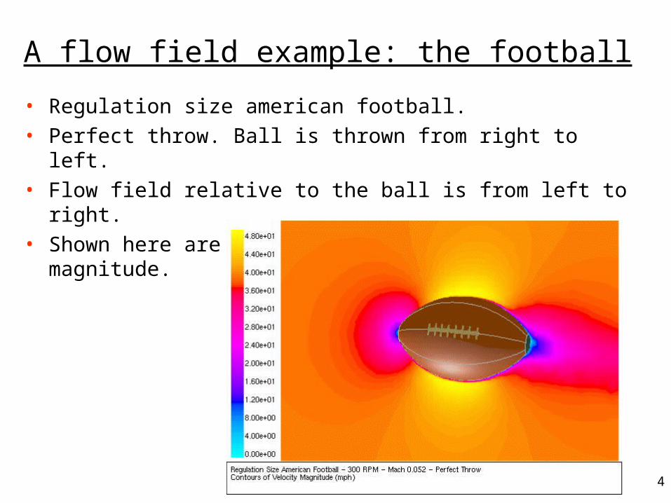
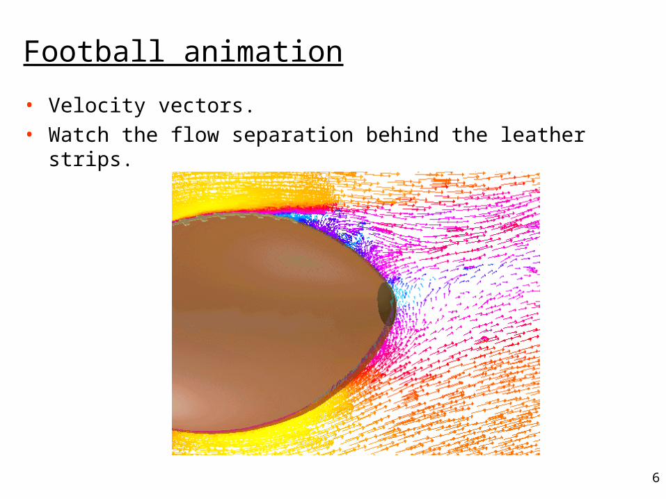
Football animation

• Time dependent calculation. Images were saved at every time step.

• Transparency for the football surface was set to 50% so that the leather strips are also visible when in the back. This helps showing the motion of the ball.

6

Football animation

• Velocity vectors.

• Watch the flow separation behind the leather strips.

Vector Plot on Iso-Surface of Constant Grid. Irregular Looking.

Vector Plot on Bounded Sample Plane. Slower but Regular Looking!

9

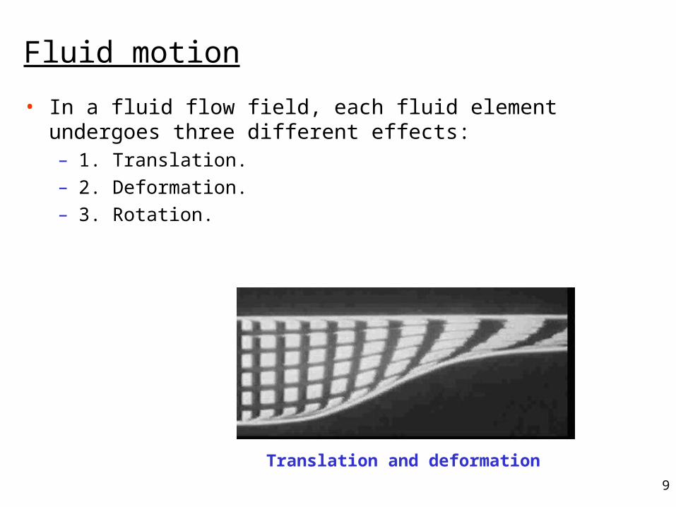
Fluid motion

• In a fluid flow field, each fluid element undergoes three different effects:– 1. Translation.– 2. Deformation.– 3. Rotation.

Translation and deformation

10

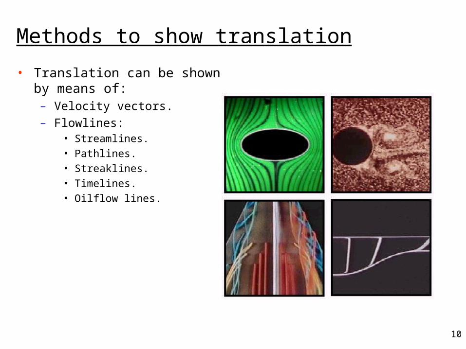
Methods to show translation

• Translation can be shown by means of:– Velocity vectors.

– Flowlines:• Streamlines.• Pathlines.• Streaklines.• Timelines.• Oilflow lines.

11

Flow around a cylinder - grid

12

Flow around a cylinder – grid zoomed in

13

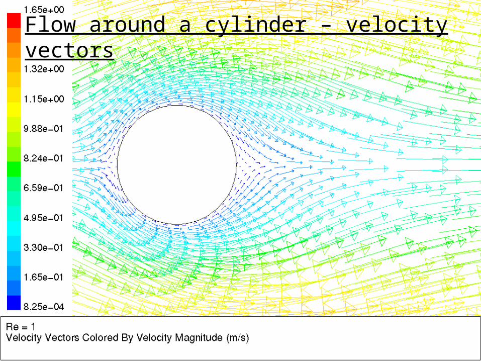
Flow around a cylinder – velocity vectors

14

Flow around a cylinder – velocity magnitude

15

Flow around a cylinder – pressure field

16

Pressure• Pressure can be used to calculate forces (e.g. drag, lift, or torque)

on objects by integrating the pressure over the surface of the object.

• Pressure consists of three components:– Hydrostatic pressure gh. – Dynamic pressure v2/2.

– Static pressure ps. This can be further split into an operating pressure (e.g. atmospheric pressure) and a gauge pressure.

• When static pressure is reported it is usually the gauge pressure only.

• Total pressure is the static pressure plus the dynamic pressure.

17

Streamlines

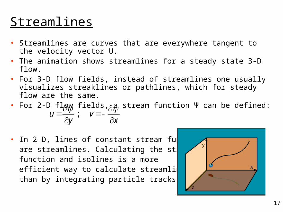
• Streamlines are curves that are everywhere tangent to the velocity vector U.

• The animation shows streamlines for a steady state 3-D flow.• For 3-D flow fields, instead of streamlines one usually visualizes

streaklines or pathlines, which for steady flow are the same.• For 2-D flow fields, a stream function Ψ can be defined:

• In 2-D, lines of constant stream functionare streamlines. Calculating the streamfunction and isolines is a moreefficient way to calculate streamlinesthan by integrating particle tracks.

xv

yu

;

18

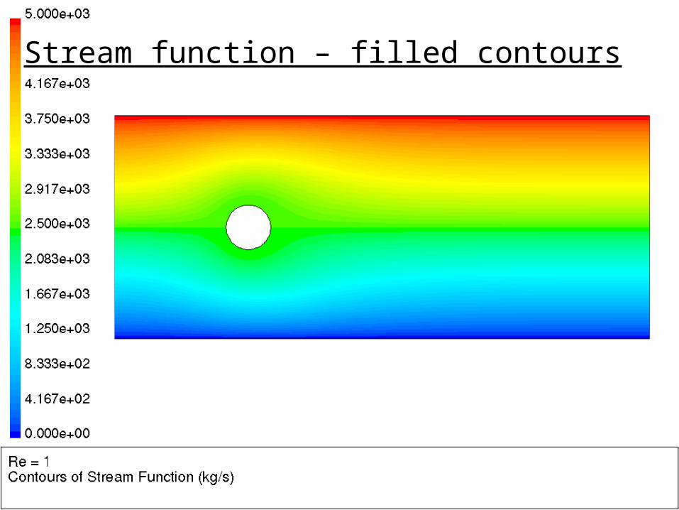
Stream function – filled contours

19

Lines of constant stream function

20

Pathlines

• A pathline is the trajectory followed by an individual particle.

• The pathline depends on the location where the particle was injected in the flow field and, in unsteady flows, also on the time when it was injected.

• In unsteady flows pathlines may be difficult to follow and not easy to create experimentally.

• For a known flowfield, an initial location of the particle is specified. The trajectory can then be calculated by integrating the advection equation:

0)0(),()(

XXXUX conditioninitalwithtdt

td

21

Pathlines

• Example: pathlines in a static mixer.

22

Pathlines around a cylinder

23

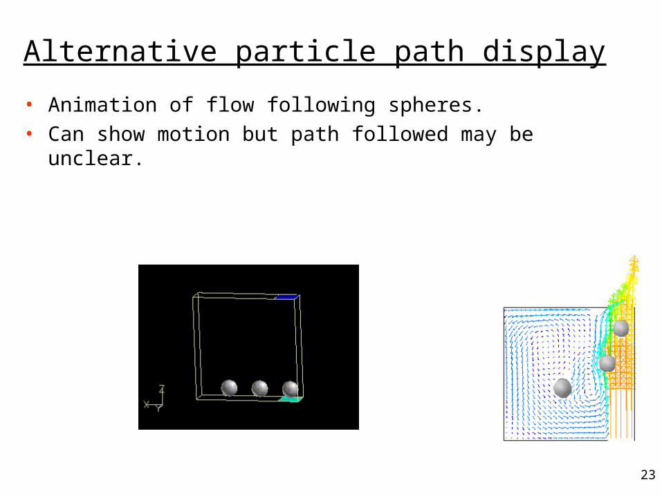
Alternative particle path display

• Animation of flow following spheres.

• Can show motion but path followed may be unclear.

24

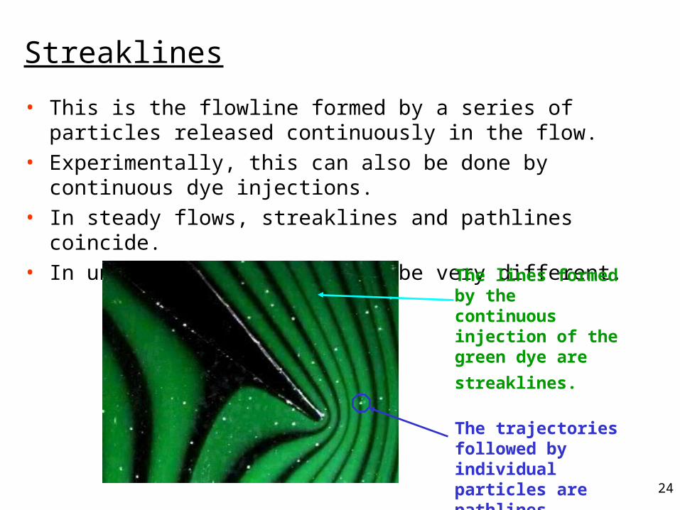
Streaklines

• This is the flowline formed by a series of particles released continuously in the flow.

• Experimentally, this can also be done by continuous dye injections.

• In steady flows, streaklines and pathlines coincide.

• In unsteady flows, they may be very different.The lines formed by the continuous injection of the green dye are

streaklines.

The trajectories followed by individual particles are pathlines.

25

Pathlines and streaklines - unsteady flow

• The animation shows a simple model of an unsteady flow coming from a smokestack.

• First, there is no wind and the smoke goes straight up.• Next there is a strong wind coming from the right.• The yellow circles show the trajectory of a single particle released at

time 0. The pathline is straight up with a sharp angle to left.• The grayish smoke shows what happens to a continuous stream. first it

goes straight up, but then the whole, vertical plume ofsmoke moves to the left.

• So, although for steady flows. pathlines and streaklines are thesame, they are not for unsteady flows.

26

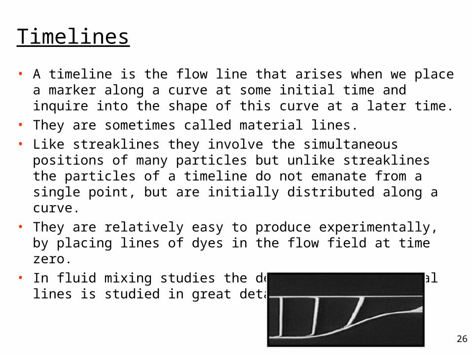
Timelines

• A timeline is the flow line that arises when we place a marker along a curve at some initial time and inquire into the shape of this curve at a later time.

• They are sometimes called material lines.

• Like streaklines they involve the simultaneous positions of many particles but unlike streaklines the particles of a timeline do not emanate from a single point, but are initially distributed along a curve.

• They are relatively easy to produce experimentally, by placing lines of dyes in the flow field at time zero.

• In fluid mixing studies the deformation of material lines is studied in great detail.

27

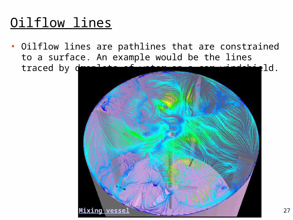
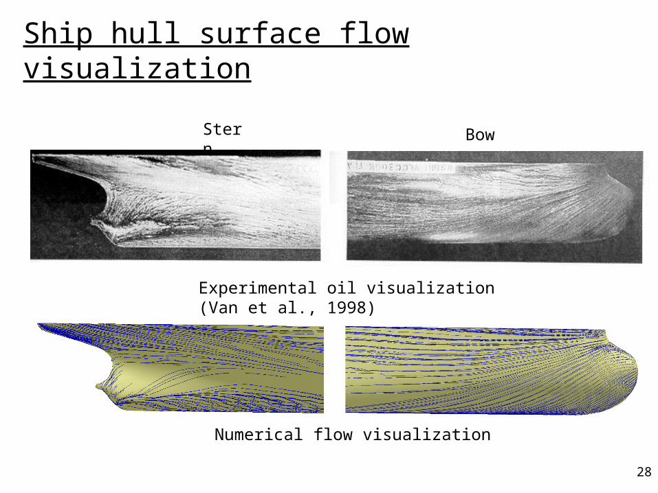
Oilflow lines

• Oilflow lines are pathlines that are constrained to a surface. An example would be the lines traced by droplets of water on a car windshield.

Mixing vessel

28

Experimental oil visualization (Van et al., 1998)

Stern Bow

Numerical flow visualization

Ship hull surface flow visualization

29

Deformation - derivatives

• An instantaneous flow field is defined by velocities u(x,y,z), v(x,y,z), and w(x,y,z).

• The derivatives are du/dx, du/dy, etc.

• The tensor u is the gradient of the velocity vector.

• Each of the terms by itself is a gradient, e.g. du/dy is the gradient of the u-velocity component in the y-direction. These may also be called shear rates.

zwywxw

zvyvxv

zuyuxu

w

v

u

z

y

x

///

///

///

/

/

/

u

30

Decomposition

• For the analysis of incompressible flows, it is common to decompose the gradient in the velocity vector as follows:

• Sij is the symmetric rate-of-strain (deformation) tensor.

Ij is the antisymmetric rate-of-rotation tensor.

• The vorticity and the rate of rotation are related by:

1

2ji

ijj i

UUS

x x

1

2ji

ijj i

UU

x x

symbolgalternatintheisijkkijkijjkijki 2

1

ijij

j

i Sx

U

31

Deformation tensor

• The velocity gradients can be used to construct the deformation rate tensor S:

• This symmetric tensor is also called the rate of strain tensor.

• Instead of the symbol S, the symbols D and E are sometimes used.

TuuS )(2

1

zw

yw

zv

xw

zu

yw

zv

yv

xv

yu

xw

zu

xv

yu

xu

21

21

21

21

21

21

S

i

j

j

iij x

u

x

uS

21

32

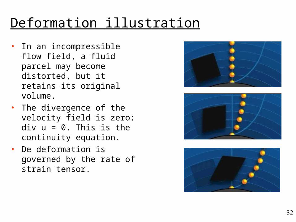
Deformation illustration

• In an incompressible flow field, a fluid parcel may become distorted, but it retains its original volume.

• The divergence of the velocity field is zero: div u = 0. This is the continuity equation.

• De deformation is governed by the rate of strain tensor.

33

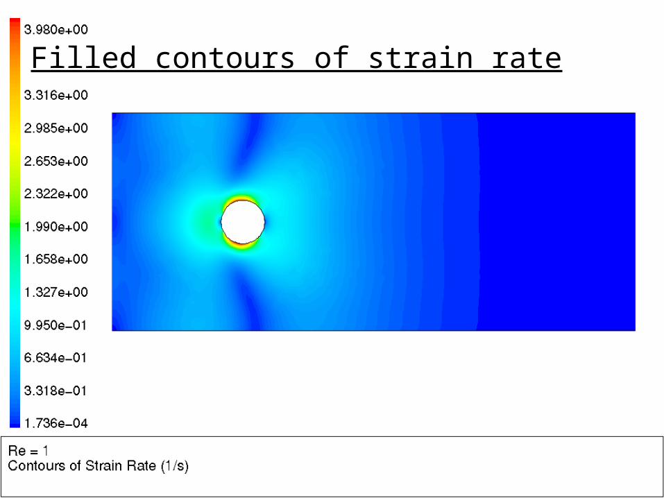
Strain rate

• The deformation rate tensor appears in the momentum conservation equations.

• It is common to report the strain rate S(1/s), which is based on the Euclidian norm of the deformation tensor:

• The strain rate may also be called the shear rate.

• The strain rate may be used for various other calculations:– For non-Newtonian fluids, the viscosity depends on the strain rate.– In emulsions, droplet size may depend on the strain rate.– The strain rate may affect particle formation and agglomeration in

pharmaceutical applications.

ijij SSS 2

34

Filled contours of strain rate

35

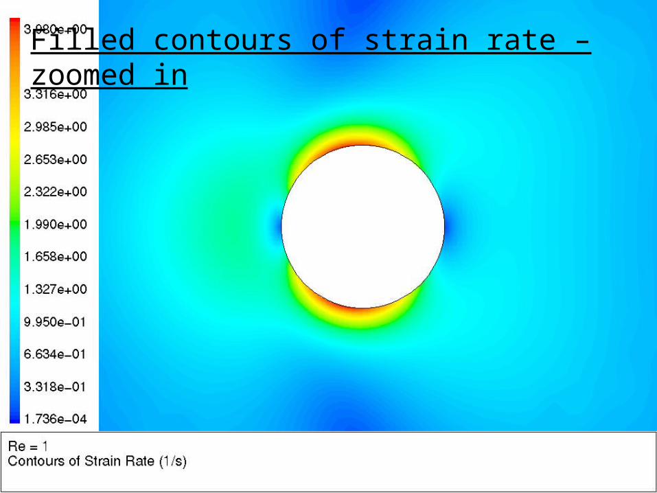
Filled contours of strain rate – zoomed in

• As discussed, the motion of each fluid element can be described as the sum of a translation, rotation, and deformation.

• The animation shows a translation and a rotation.• Vorticity is a measure of the degree of local rotation in the fluid. This is a

vector. Unit is 1/s. • For a 2-D flow this vector is always normal to the flow field plane.• For 2-D flows, vorticity is then usually reported as the scalar:

• For 2-D flows, a positive vorticity

indicates a counterclockwise rotation

and a negative vorticity a clockwise

rotation.

Vorticity

yu

xv

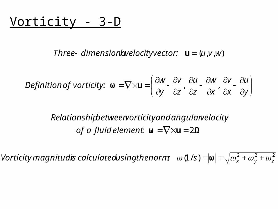
Vorticity - 3-D

222)/1(

2:

,,

),,(

zyxs:normtheusingcalculatedismagnitudeVorticity

elementfluidaof

velocityangularandvorticitybetweenlationshipRe

y

u

x

v

x

w

z

u

z

v

y

wvorticity:ofDefinition

wvu:vectorvelocityldimensionahreeT

ω

Ωuω

uω

u

38

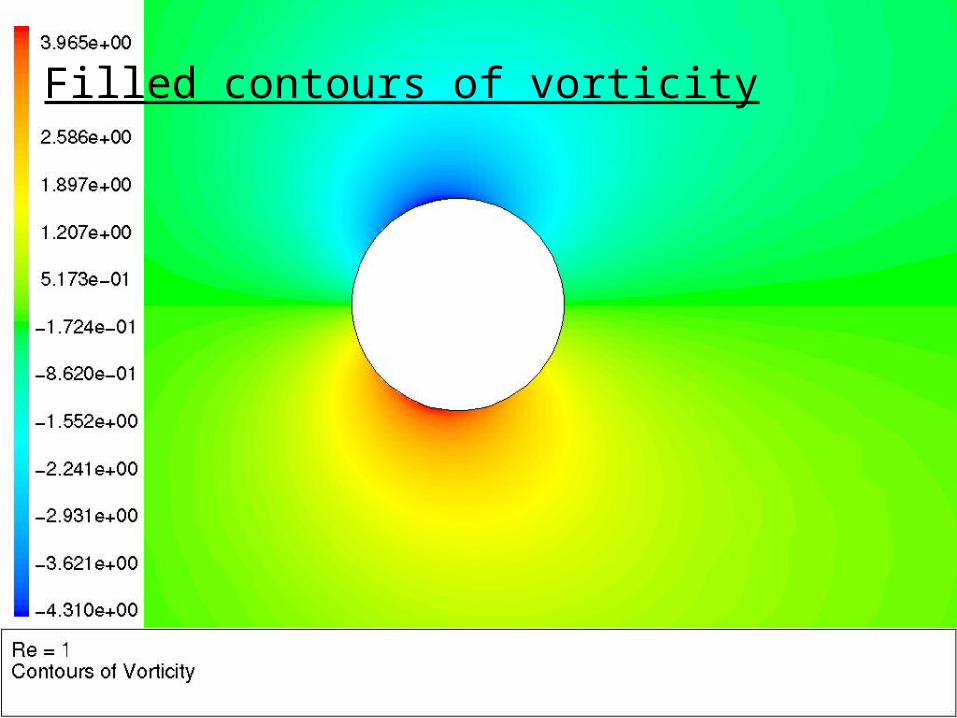
Filled contours of vorticity

39

H ω U

|))||/(|(cos 1 UωH

Vortexlines and helicity

• Iso-surfaces of vorticity can be used to show vortices in the flow field.

• Vortex lines are lines that are everywhere parallel to the vorticity vector.

• Vortex cores are lines that are both streamlines and vortexlines.

• The helicity H is the dot product of the vorticity and velocity vectors:

• It provides insight into how the vorticity vector and the velocity vector are aligned. The angle between the vorticity vector and the velocity vector (which is 0º or 180º in a vortex core) is given by:

• Algorithms exist that use helicity to automatically find vortex cores. In practice this only works on very fine grids with deeply converged solutions.

40

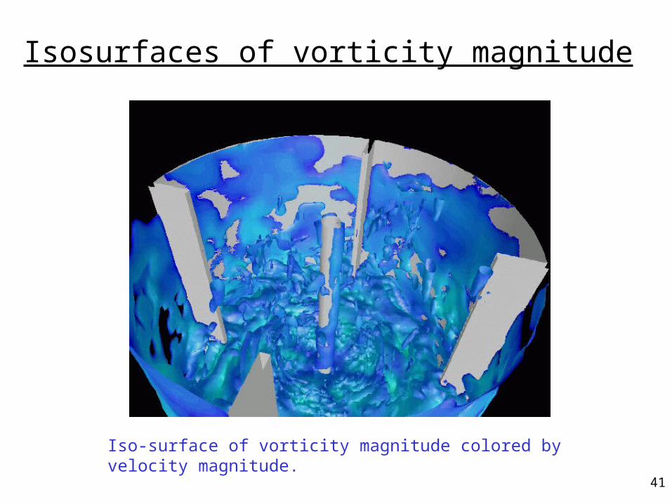
Isosurfaces of vorticity magnitude

Iso-surface of vorticity magnitude colored by velocity magnitude.

41

Isosurfaces of vorticity magnitude

Iso-surface of vorticity magnitude colored by velocity magnitude.

42

Comparison between strain and vorticity

• Both strain and vorticity contain velocity gradients.

• The difference between the two will be shown based on three different flow fields:– A planar shear field: both the strain rate and the vorticity magnitude

are non-zero.– A solid body rotation: the strain rate is 0(!) and the vorticity reflects

the rotation speed.– Shear field and solid body rotation combined.

43

A planar shear field

44

Solid body rotation

45

Shear field and solid body rotation combined

46

Flux reports and surface integrals

• Integral value:

• Area weighted average:

• Mass flow rate:

||1

i

n

ii AdA

||11

1i

n

ii A

AdA

A

iii

n

ii AnVdAnV ).().(

1

47

• Turbulent simulation (using RNG and 170,000 tetrahedral cells) is used to predict the near-body pressure field.

Quantitative validation - moving locomotive

48

• Pressure contours show the disturbance of the passing train in the near field region.

• The figure on the left shows the pressure field over the locomotive.• Predictions of pressure coefficient alongside the train agree reasonably

well with experimental data.

Flow over a moving locomotive

49

• The surrounding fluid exerts pressure forces and viscous forces on the airfoil:

• The components of the resultant force acting on the object immersed in the fluid are the drag force and the lift force. The drag force D acts in the direction of the motion of the fluid relative to the object. The lift force L acts normal to the flow direction.

• Lift and drag are obtained by integrating the pressure field and viscous forces over the surface of the airfoil.

p < 0U

p > 0

Uw

L i f t D r a g

22

2

1..

2

1.. UACDUACL DL

Quantitative validation - NACA airfoil

50

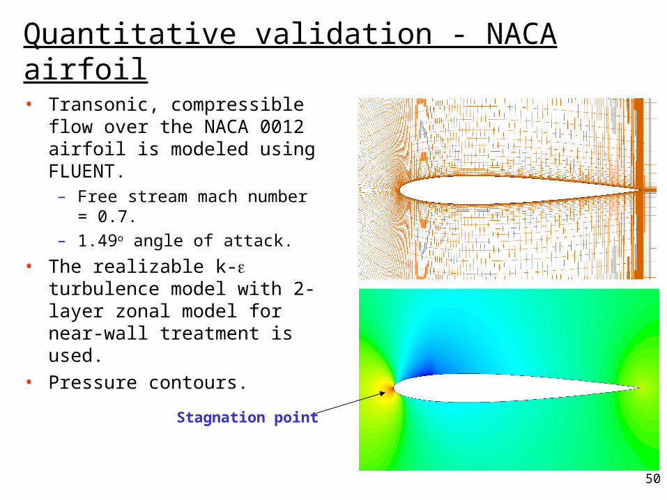
Quantitative validation - NACA airfoil

• Transonic, compressible flow over the NACA 0012 airfoil is modeled using FLUENT.– Free stream mach number = 0.7.

– 1.49o angle of attack.

• The realizable k- turbulence model with 2-layer zonal model for near-wall treatment is used.

• Pressure contours.

Stagnation point

51

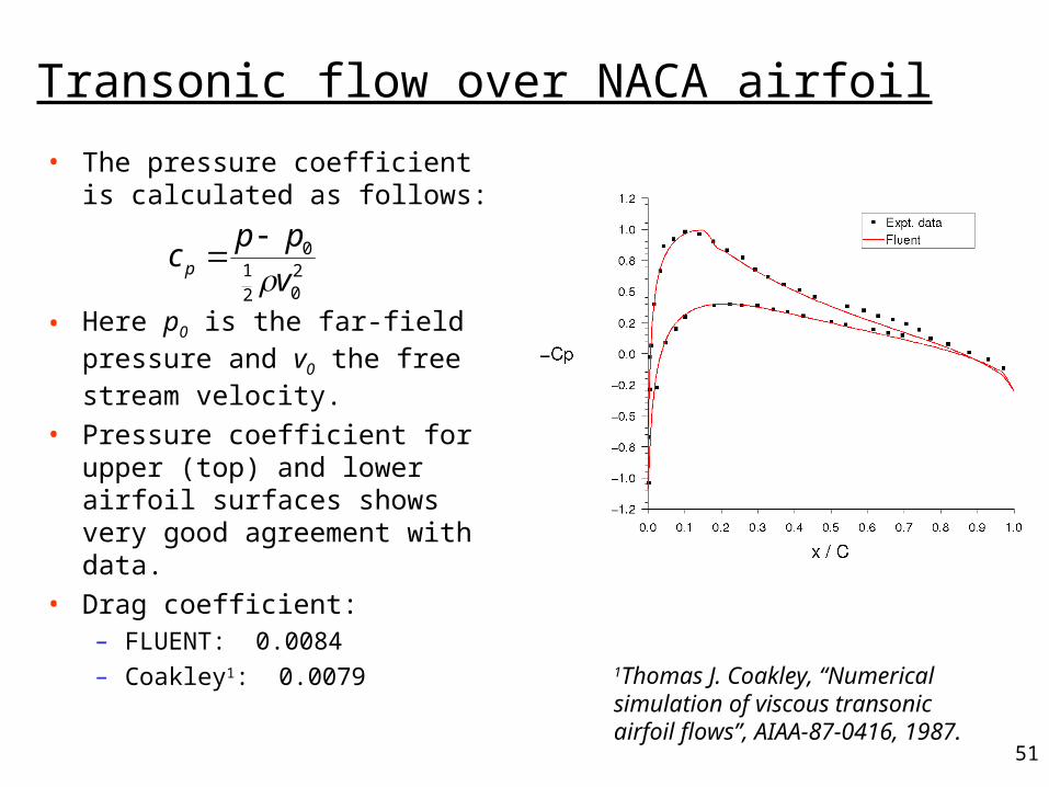
• The pressure coefficient is calculated as follows:

• Here p0 is the far-field pressure and v0 the free stream velocity.

• Pressure coefficient for upper (top) and lower airfoil surfaces shows very good agreement with data.

• Drag coefficient:– FLUENT: 0.0084

– Coakley1: 0.00791Thomas J. Coakley, “Numerical simulation of viscous transonic airfoil flows”, AIAA-87-0416, 1987.

Transonic flow over NACA airfoil

202

10

v

ppc p

52

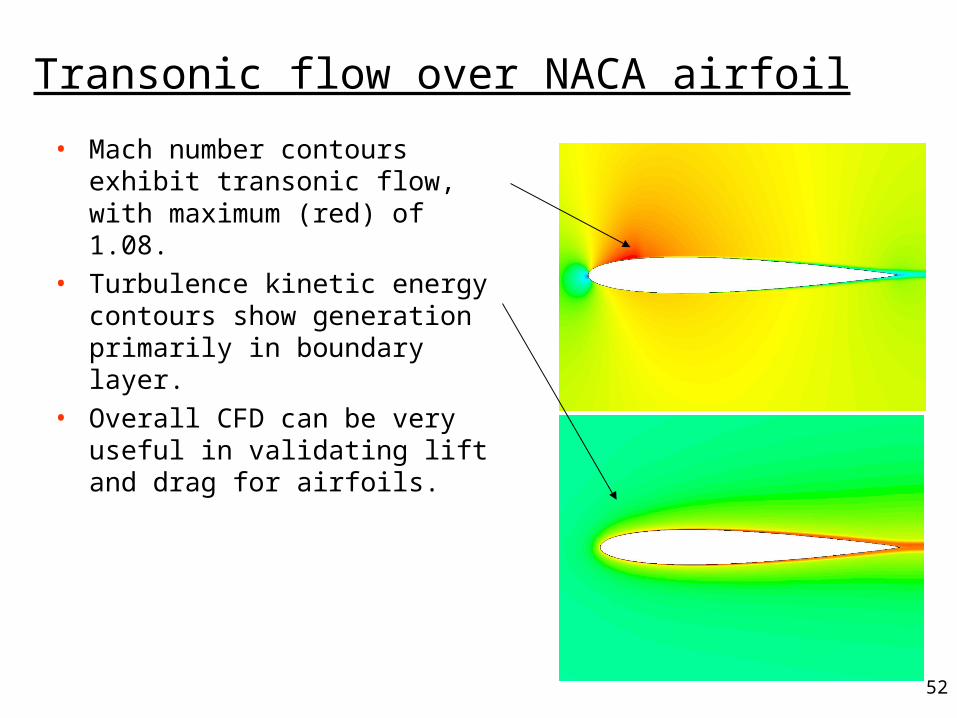
• Mach number contours exhibit transonic flow, with maximum (red) of 1.08.

• Turbulence kinetic energy contours show generation primarily in boundary layer.

• Overall CFD can be very useful in validating lift and drag for airfoils.

Transonic flow over NACA airfoil

53

Summary

• CFD simulations result in data that describes a flow field.

• Proper analysis and interpretation of this flow field data is required in order to be able to solve the original engineering problem.

• The amount of data generated by a CFD simulation can be enormous. Analysis and interpretation are not trivial tasks and the time it takes to do this properly is often underestimated.