1

Joint Source-Channel Coding

using Real BCH Codes

for Robust Image TransmissionA. Gabay1, M. Kieffer2,∗, and P. Duhamel2

1 Bloophone S.A., 96 Bd de sebastopol, F-75003 Paris

France Phone: 00 33 1 44 54 05 50, Fax : 00 33 1 44 54 05 15

a.gabay@bloophone.com2 LSS – CNRS – Supelec – Universite Paris-Sud

Plateau de Moulon, F-91192 Gif-sur-Yvette, France

Phone: 00 33 1 69 85 17 32, Fax : 00 33 1 69 85 17 65

{michel.kieffer,piere.duhamel}@lss.supelec.fr

Abstract

In this paper, a new still image coding scheme is presented. In contrast with standard tandem

coding schemes, where the redundancy is introduced after source coding, it is introduced before

source coding using real BCH codes. A joint channel model is first presented. The model corresponds

to a memoryless mixture of Gaussian and Bernoulli-Gaussiannoise. It may represent the source coder,

the channel coder, the physical channel, and their corresponding decoder. Decoding algorithms are

derived from this channel model and compared to a state-of-art real BCH decoding scheme. A further

comparison with two reference tandem coding schemes and theproposed joint coding scheme for the

robust transmission of still images has been presented. When the tandem scheme is not accurately

tuned, the joint coding scheme outperforms the tandem scheme in all situations. Compared to a

tandem scheme well-tuned for a given channel situation, thejoint coding scheme shows an increased

robustness as the channel conditions worsen.

EDICS Category: COM-SOUR,COM-ERRO

I. INTRODUCTION

The classical approach to solve the problem of reliably sending compressed images or video over

a noisy channel is to use atandemsource-channel coding (TSCC) scheme. Redundancy is inserted

∗ Corresponding author

Parts of this work have been presented at Globecom 2000 [1], ICASSP 2001 [2], ICC 2002 [3], and ICC 2003 [4]

July 30, 2006 DRAFT

2

at the output of the source coder by a channel coder with the intent that the channel decoder will

detect and correct all erroneously received data. Thus, protecting against errors results in an increase

in bandwidth. Sometimes however, the channel decoder is notable to correct all transmission errors,

due to complexity or delay constraints, for example, and this results in highly corrupted reconstructed

data with almost all efficient source encoders. On the contrary, if the channel is not too noisy, the

excess bandwidth required by channel coding is wasted sincethe channel decoder does not consider

the distortions introduced by source coding. The problem here is that classical communication systems

are tuned for a precise target situation, and that a deviation of this situation from the nominal one

may result in suboptimality.

Shannon’s classical separation result states that the end-to-end performance of a transmission

scheme can be optimized by separately optimizing the sourceencoder-decoder pair and the channel

encoder-decoder pair [5]. However, this result holds only in the limit of infinite channel code block

length and for stationary channels, two assumptions that are seldom met in practical situations such

as mobile or satellite transmission: usually the delay is constrained, which makes the infinite block

length assumption unreasonable, and the channels may be quite different at various locations, thus

hitting the stationarity assumption. Furthermore, Shannon’s theory does not provide a design algorithm

for good channel codes with finite block length. In addition,it does not address the design of good

source codes when the probability of channel error is non-zero, which is unavoidable for finite-length

channel codes. Thus, for practical systems, in which the delay or complexity is constrained, a joint

source and channel code design may reduce distortion.

In the last years, Joint Source-Channel Coding (JSCC) received an increasing interest in the research

community, while having difficulties to enter practical applications. In [6], an overview of the various

techniques available before 1996 may be found. Today, JSCC embeds a large variety of techniques

which share the common property of not applying Shannon’s separation principle. Albeit the frontiers

between techniques are not so clear, one may distinguish four main families of techniques.

- In concatenated codingschemes, the Source Coder (SC) and Channel Coder (CC) are twoseparate

units which are jointly optimized in order to get a minimum distortion for a given bitrate. Unequal

error protection is the most commonly used technique of thisfamily. Subband image coders or hybrid

video coders [7] generate informations which can be groupedin classes according to their sensitivity

to noise. Very sensitive data are strongly channel encoded whereas weak channel codes are used for

the less sensitive data. See,e.g., [8] for a technique using mainly the modulation and [9], [10] for

CC which may easily be adapted to channel conditions or data sensitivity.

- In schemes where thesource coder is optimized for the channel conditions, the channel is explicitly

taken into account in the design of the SC. First results havebeen obtained by [11], who optimizes

the index assignment in order to mitigate the effect of errors introduced by the channel. Multiple

description schemes also belong to this family. More precisely, the idea is to optimize the redundancy

July 30, 2006 DRAFT

3

between descriptions with the channel conditions, see,e.g., [12]. Entropy codes with error-detecting

or correcting capabilities also belongs to this family, see[13] for reversible variable-length codes and

[14], [15] for variable-length codes optimized according to the channel conditions.

- In joint decodingschemes, information provided by the channel decoder is used to improve the

decoding realized by the source decoder [16]. All techniques belonging to this family use the fact

that the source coder leaves some redundancy in the bitstream to perform a decoding using channel

decoding techniques. In [21], a MAP detection schemes is proposed to mitigate transmission errors,

taking the redundancy of images into account via a second-order Markov process. This requires the

accurate transmission of the Markov model to the receiver. In [22], a Baum-Welch algorithm is put

at work to perform jointly the decoding and the estimation ofthe parameters of a hidden Markov

model for a binary source. See also [17]–[20] for decoding ofvariable-length encoded data using

residual source redundancy.

- In joint coding schemes, the location of the CC or even the distinction between SC and CC

is not clear anymore. Punctured convolutional codes have been used to realize source coding [23].

The choice of the puncturing matrix makes it possible to smoothly transform a CC in a SC [24],

[25]. In a similar flavor, [26] realize the SC and CC with nonlinear transforms with dimensionality

change inspired from [27]. A dimension increase corresponds to a channel coding whereas a decrease

corresponds to a source coding.

The solution proposed in this paper belongs to the latter family. It consists in using a JSCC scheme

which introduces redundancybeforesource coding using real BCH codes. The main advantage of this

technique is the ability of the joint source-channel decoder (JSCD) to correct large errors resulting

from non perfect transmissionas well asreducing the level of errors resulting from source coding. Real

BCH codes have been introduced in [28], [29], where the analogy between real-valued and finite-field

block codes is established. It will be clear from Section III-C that the main difficulty with real-number

codes in this situation comes from finite-precision computation and quantization of the encoded data.

Some entries of the data block to be decoded may be affected bysome high amplitude perturbations

(impulse noise), butall components suffer from quantization or computation noise (background noise).

In [30], the background noise is neglected and the Berlekamp-Massey (BM) and Forney [31] decoding

algorithms for finite-fields BCH codes are directly transposed to real-valued DCT codes, a subclass of

which are real BCH codes. However, in actual coding schemes,the background noise is unavoidable.

Thus, the error-correcting algorithms developed for finite-field BCH codes cannot be used directly.

In [32], a decoding technique derived from the Peterson, Gorenstein, Zierler (PGZ) algorithm is

applied for burst of erasures recovery. Erasures locationsare assumed to be known. An analysis

of the perturbation introduced by the background noise is also provided. The background noise is

explicitly taken into account in [33], where an error correcting technique based on Wiener estimation

is provided. The unknown impulse error locations are estimated using a multiple hypotheses test.

July 30, 2006 DRAFT

4

However, the corresponding results would clearly benefit from an accurate channel model describing

the part of the communication scheme lying between the real BCH encoder and decoder. At the same

time, [1] and [2] propose a Gaussian-Bernouilli-Gaussian (GBG) channel model derived from [34] to

efficiently represent ajoint channelconsisting of a scalar quantizer followed by a binary symmetric

channel and the corresponding inverse quantizer. The decoding is performed by a modified version

of the PGZ algorithm presented in [35] and taking into account the information provided by the

channel model. This technique has been improved using a multiple hypotheses test for estimating the

number of impulse errors [4] and by realizing ana posterioricontrol of the correction technique [3],

which are computationally less demanding than the techniques presented in [33]. Further results on

real BCH codes have been obtained for code vectors corruptedby bursts of erasures (with known

locations) in [36] where the background noise is taken into account. In [37], real BCH codes are

embedded in the theory of real-valued frames, which allow a further analysis of the influence of the

background noise on erasure recovery.

It has to be noted that the proposed approach is complementary to that proposed,e.g., in [16],

[21], [22]. Real BCH decoding is performedafter all other decoding techniques have done their work,

since the real BCH decoder is situated at the end of communication chain. The best the intermediate

channel or joint-source-channel techniques will perform,the best the real BCH decoder will work

too. Moreover, one of the unique specificity of real BCH codesis their ability to mitigate part of the

noise introduced by the source coder.

The aim of this paper is to summarize and complement results partly presented by the authors in

conference papers [1]–[4] on the use of real BCH codes for robust image transmission over realistic

satellite channels. It will be shown that in many practical situations, a GBG model is well suited to

represent the part of the communication scheme between the output of the real BCH coder and the

input of the real BCH decoder. Thus, data encoded using a realBCH code are affected in the channel

by a mixture of Gaussian background noise and impulse noise with Gaussian distributed amplitude.

Three problems have then to be solved: (i) determining whether an encoded vector is affected by

some impulse error and estimating their number; (ii) determining the amplitude and location of the

impulse errors; (iii) realizing the correction and verifying its efficiency. Compared to the conference

papers, a detailed presentation of the GBG channel model is provided, its capacity is evaluated and

non-trivial illustrative examples are treated. A comparison of the proposed decoding technique to a

state-of-art real BCH decoder is performed. Moreover, the usefulness of such techniques in practical

satellite image transmission situations is evaluated. Obviously, these results can be extended to more

general wireless communication channels.

The joint channel model is the key issue of the presented technique. Thus Section II is devoted

to the description and analysis of the joint GBG channel model. In Section III, properties of real

BCH codes are recalled, and coding and decoding techniques are presented. The way real BCH codes

July 30, 2006 DRAFT

5

may be introduced in actual still image coding schemes is considered in Section IV. Finally, some

examples are presented in Section V.

II. JOINT CHANNEL MODEL

In standard channel coding, the channel is the part of the communication scheme that lies between

the channel coder and the channel decoder. Similarly, for joint source-channel coding, define thejoint

channel as the part of the communication scheme between the JSCC and the JSCD, see Figure 1.

A model of the joint channel is required to be able to evaluatethe performance a JSCC/JSCD may

attain and to simplify its design. Since it is a joint channel, the model has to account for the distortion

introduced both by the source coder-decoder and the transmission.

Quantiz.Channelcoding

Channel

Source

Reconst.source

JSCC

JSCDInversequantiz.

Channeldecoding

Joint channel

Fig. 1. Definition of the joint channel

A. Introduction

Assume that a source of probability density function (pdf)p (s) generates vectorss = (s1 . . . sL)T ∈RL which pass through a quantizer defined by(i) a dictionaryD = {d1 . . .dM}, (ii) a partition

P = {P1 . . . PM} of RL in M non-overlapping regions and(iii) a functionQ such that

Q (s) = dj if s ∈ Pj , j = 1, . . . ,M.

A binary index i = I (d) is associated to the code vectord via the indexing functionI (·) and is

transmitted on a channel, which is assumed to be memoryless and characterized by its transition

probability p (ik|ij) or p (dk|dj). At receiver side, if the received index isi, the estimate for the

source vectors is s = I−1 (i) ∈ D. The distortion introduced by the quantizer and the channelis

then

D =1

L

M∑

j=0

M∑

k=0

p (dk|dj)

∫

Pj

p (s) d (s,dk) ds, (1)

whered (s,dk) is the distortion measure betweens anddk, see [11].

When the distortion measure is the quadratic euclidean norm, then(1) may be written as

D = E(|s− s|2

)= E

(|s− Q (s)|2

)+ E

(|Q (s) − s|2

)+ 2.E

((s − Q (s))T . (Q (s) − s)

). (2)

July 30, 2006 DRAFT

6

The first term in (2) corresponds to the distortion introduced by the quantizer,the second, to

the distortion introduced by the channel and the last one to the mutual distortion. For well-tuned

quantizers, the last term can be neglected [38] to get

D ≈ E(|s− Q (s)|2

)+ E

(|Q (s) − s|2

). (3)

B. New channel model

The joint channel model has to account for both types of distortion expressed in(3). The proposed

Gaussian-Bernoulli-Gaussian(GBG) channel model [34] consists of a memoryless channel corrupted

by a mixture of Gaussian noise with small variance and of Bernoulli-Gaussian (BG) noise. The

Gaussian noise models the quantization noise and corresponds to the first term of(3). The BG

noise represents the channel errors that were not correctedby the channel coder/decoder pair and

corresponds to the second term of(3).

Assume that the inputc (k) and outputr (k) of the joint channel are related by

r (k) = c (k) + b (k) + γ (k) (4)

whereb (k) is zero-mean Gaussian with varianceσ2g andγ(k) = ξ(k)ηi(k) is a BG noise withξ(k)

a Bernoulli process,i.e., an i.i.d. sequence of zeros and ones with Prob(ξ(k) = 1) = pi , andηi(k) is

zero-mean Gaussian with varianceσ2i . Obviously, in most situations,σ2

i >> σ2g since channel errors,

when they occur, impact much more significantly on the distortion than quantization noise.

The pdf associated withγ(k) is

p (γ) = (1 − pi) δ (γ) + pi(2πσ2

i

)−1/2exp

(− γ2

2σ2i

). (5)

The pdf ofη (k) = b (k) + γ (k) is thus a convolution of a Gaussian pdf and of(5)

p (η) = (1 − pi)(2πσ2

g

)−1/2exp

(− γ2

2σ2g

)+ pi

(2π(σ2

g + σ2i

))−1/2exp

(− γ2

2(σ2

g + σ2i

))

. (6)

This model may seem quite rough, since it is well known, for example, that quantization noise is

far from being Gaussian, but it is shown in Section II-C that it can describe quite accurately many

practical situations.

This GBG joint channel model is thus characterized by three parameterspi , σ2g andσ2

i which have

to be estimated for a given channel. They may be obtained in three steps.

1) First evaluate the distortionDq introduced by the source coder assuming that the channel is

error-free. This distortion is modeled by the Gaussian partof the GBG model. An estimate of

the variance of the Gaussian noise may then be chosen asσ2g = Dq.

2) Then consider the noise introduced by the channel and evaluate the probability that a sample

is in error after source decoding, as a function of the channel, the channel coder-decoder, and

July 30, 2006 DRAFT

7

the source coder-decoder parameters. This leads to an estimate pi of the parameterpi in the

BG noise.

3) Finally, evaluate the distortionDi introduced by the channel error on the reconstructed samples

after source decoding. Using(5), the distortion introduced by the BG noise would be

Di = (1 − pi)

∫ +∞

−∞γ2δ (γ) dγ + pi

∫ +∞

−∞γ2(2πσ2

i

)−1/2exp

(− γ2

2σ2i

)dy = piσ

2i . (7)

An estimate of the variance of the Gaussian noise in the BG noise may be obtained as

σ2i = Di/pi . (8)

C. Examples

The accuracy of the proposed model is verified below through some examples. Another example

may be found in Appendix I.

1) Scalar quantizer followed by a BSC:Consider a sources quantized by anM = 2b levels scalar

quantizer before being transmitted over a memoryless BSC with transition probabilityε. The scalar

quantizer, with dictionaryD = {d1, . . . , dM}, introduces a distortionDq = E(|s − Q (s)|2

), which

may be modeled by the zero-mean Gaussian noiseb in (4) of variance

σ2g = Dq. (9)

The BSC introduces additional distortion, since bit errorson the channel result in index errors at

the decoder. The transition probabilityp (ik|ij) = p (dk|dj) may be expressed as

p (ik|ij) = εdH(ij ,ik) (1 − ε)b−dH(ij,ik) , (10)

where dH (·, ·) stands for the Hamming distance. Using(10) and taking into account the source

decoder, the distortion between the quantizer outputd and its estimated after source decoding may

be written as

Di = E

(∣∣∣d − d∣∣∣2)

=

M∑

j=1

M∑

k=1

εdH(ij ,ik) (1 − ε)b−dH(ij,ik) p (dj) |dj − dk|2 , (11)

An estimate for the probabilitypi of the GBG model is the probability that an index is in error

pi = 1 − (1 − ε)b . (12)

By combining (8), (11) and (12), one then gets an estimate for the parameterσ2i of the GBG

model

σ2i =

∑Mj=1

∑Mk=1 p (dj) εdH(ij ,ik) (1 − ε)b−dH(ij ,ik) p (dj) |dj − dk|2

1 − (1 − ε)b. (13)

For a zero-mean unit-variance Gaussian source, Figure 2 illustrates the evolution ofσ2i /σ

2g as a

function of the bitrateb for a given transition probabilityε = 10−2 of the BSC. This ratio does not

significantly depend of the type of quantization used (uniform and non uniform scalar quantizers).

July 30, 2006 DRAFT

8

1 2 3 4 5 6 7 85

10

15

20

25

30

35

40

45

50

b

Uniform Scalar QuantizationNonuniform Scalar Quantization

10lo

g(

)10

¾¾

ig

²²

/

Fig. 2. Relation between quantization and impulse noise variances for uniform and nonuniform scalar quantization followed

by a BSC withε = 10−2

For a scalar quantizer followed by a BSC, consideringγ as a high amplitude impulse noise compared

to the quantization noise is thus quite reasonable, even at low bitrates.

A comparison of the input-output behavior of a joint channelconsisting of a nonuniform scalar

quantizer followed by a BSC and an inverse quantizer versus its GBG model is represented on

Figure 3. A zero-mean unit-variance Gaussian source has been quantized onM levels, with M ∈{21, 22, 24, 26

}. For all quantizers, the difference between the actual channel and its model is less

0

10

20

30

40b = 6 bits/sample

0

5

10

15

20

25

b = 4 bits/sample

2

4

6

8

10

b = 2 bits/sample

2

2.5

3

3.5

4

4.5b = 1 bit/sample

"

End t

o en

d S

NR

(dB

)

10-5

10-4

10-3

10-2

10-1

10-5

10-4

10-3

10-2

10-1

10-5

10-4

10-3

10-2

10-1

10-5

10-4

10-3

10-2

10-1

Fig. 3. Comparison of a joint channel (*) and its GBG model (o)as a function ofε (scalar quantization followed by a

BSC and an inverse quantization).

than2 dB. Moreover, belowε = 10−3, it is less than0.5 dB, except forM = 26 where it is about

1 dB. This shows that the GBG model is realistic for a large interval of ε and for many scalar

July 30, 2006 DRAFT

9

quantizers. The differences come from the fact that, at highvalues ofε, the quantization noise and

the noise introduced by the channel are correlated and the third term in (2) should not be neglected,

see [11], [39].

2) Scalar quantization associated with anMPSK followed by an AWGN channel:Consider the

same sources that passes through the same scalar quantizer but now followed by anMPSK sending

bits over an AWGN channel characterized by its varianceN0/2. In the signal space,M points

{u1, . . . ,uM} form the constellation of theMPSK.

An estimate of the first parameterσ2g of the GBG model(6) is still given by (9).

Assuming thatuj corresponds to the output leveldj of the scalar quantizer, the probability of

transition fromuj to uk may bounded as [40]

p (uk|uj) 6erfc

(|uj − uk| /

(2√

N0

))

2. (14)

An estimate ofpi in the GBG model is then obtained by using the union bound [40]and by averaging

all transition probabilities(14) to get

pi =M∑

j=1

p (dj)M∑

k=1,k 6=j

erfc(|uj − uk| /

(2√

N0

))

2. (15)

The resulting distortion between the quantizer outputd and its estimated after demodulation and

source decoding is

Di = E

(∣∣∣d − d∣∣∣2)

=

M∑

j=1

M∑

k=1,k 6=j

p (uk|uj) p (dj) |dk − dj |2 . (16)

An estimate of the variance of the Gaussian part of the BG process may again be evaluated using

(8), (15) and(16)

σ2i =

∑Mj=1

∑Mk=1,k 6=j erfc

(|uj − uk| /

(2√

N0

))p (dj) |dk − dj|2

2∑M

j=1 p (dj)∑M

k=1,k 6=j

erfc(|uj−uk|/(2√

N0))2

(17)

To verify the accuracy of this model, consider a zero-mean unit-variance Gaussian source quantized

using anM levels non-uniform scalar quantizer. Its output indexes are mapped on anMPSK and sent

over an AWGN channel followed by an ML receiver and an inversequantizer. Figure 4 compares the

performance of the joint channel and of its GBG model whenM = 23 andM = 24.

In both cases, except at lowEb/N0, where the GBG channel is more pessimistic (mostly due to the

pessimism of the union bound), the GBG model is again quite realistic to represent the perturbations

introduced by the quantization, modulation and channel.

3) Influence of a channel coder:In the previous examples, no channel coder has been considered.

The easiest way to account for its influence is to build an equivalent BSC channel model of the group

formed by the channel coder, channel and channel decoder. A new transition probabilityε′ may be

evaluated and all previous computations may be performed ina similar way.

July 30, 2006 DRAFT

10

0

5

10

15

En

d t

o E

nd

SN

R

10-5

100

p

14

15

16

17

Eb/N

0E

b/N

0

8-PSK 16-PSK

0

10

20

10-4

10-2

100

10

15

20

25

10lo

g(

)10

¾¾

ig

²²

/

0 2 4 6 8 10 12 14 160 2 4 6 8 10 12 14

Fig. 4. Comparison of a joint channel (*) and its GBG model (o), (M = 23 and M = 24 levels scalar quantization

followed by anMPSK, an AWGN channel, an ML receiver and an inverse quantization)

D. Channel capacity

Using the Arimoto-Blahut algorithm [41], it is possible to compute the capacity of the GBG joint

channel model for variouspi or σ2i /σ

2g. In the considered case,σ2

g = 10−1 andσ2i = 1. For various

values ofpi ∈{10−3, 10−2, 5.10−2, 10−1

}, the capacity is plotted on Figure 5 as a function of the

input signal powerP . The AWGN channel is the reference corresponding topi = 0.

1 2 3 4 51

1.5

2

2.5

3

Cap

acity (

bit

/s/H

z)

P

Gaussian channel

GBG channel, pi= 10-3

GBG channel, pi= 10-2

GBG channel, pi= 5.10-2

GBG channel, pi= 10-1

Fig. 5. GBG channel capacity as a function of the input signalpowerP, for variousp (σ2

q = 0.1, 10 log10

σ2i

σ2q

= 10 dB)

For a moderate input signal power, even with the quite high impulse error probability of10−2, the

channel capacity remains very similar to that of an AWGN channel. This suggests that a well-designed

JSCC/JSCD may mitigate the effect of impulse errors in the GBG channel.

July 30, 2006 DRAFT

11

E. Comments on the channel model

The purpose of this section was to show that, despite the complexity of the global system, a GBG

channel model could describe the impact of the source codingplus that of the residual transmission

errors with a very good accuracy in most cases, and could at least give an order of magnitude of

the global distortion depending on the system parameters. This is a key point in our approach, and

represents one of the main differences with [33], since we heavily rely on this simple model to build

efficient decoders.

Note also that our channel model clearly imposes a precise definition of what anerror is. Because

of the presence of a Gaussian noise on all samples and becausethe emitted signal is continuous, there

is no hope that this background noise can be corrected. However, one can hope to get rid of the BG

part, which has few contributions (in terms of erroneous samples). Thus, theerror correction capacity

in what follows refers to the ability to correct impulse errors, despite the presence of background

noise.

III. R EAL BCH CODES

This section briefly recalls BCH codes on the real field. Encoding and decoding techniques are

presented. The way they may be incorporated in JSCC/JSCD schemes to mitigate the effect of a GBG

channel is also illustrated.

A. Definition

The definitions of spectral and BCH codes over finite fields given,e.g., in [31] may be translated to

define BCH(n, k) codes over the real field (real BCH(n, k) codes) as spectral codes whose elements

belong toRn and are such that their spectrum vanishes over a set ofconsecutive parity frequencies

A = {a0, . . . , a0 + n − k − 1} ,

satisfying for allf ∈ A, n − f ∈ A, and wherea0 is the base index, see [29], [33].

Various techniques may be employed to perform a real BCH(n, k) encoding. One could think of

polynomial constructions inspired from classical finite fields cyclic codes. This paper focuses on the

spectral interpretation and construction of real BCH(n, k) codes withk odd. Our construction also

includes some properties that will be useful in our context (interpolation property).

Consider areal information vectorxk ∈ Rk, an associated BCH(n, k) code vectorcn ∈ Rn may

be built as follows

cn = WnPn,kW−1k xk, (18)

whereWn is then−dimensional discrete Fourier transform matrix and where

Pn,k =

I⌈n/2⌉−t 0⌈n/2⌉−t,k−⌈n/2⌉+t

0n−k,⌈n/2⌉−t 0n−k,k−⌈n/2⌉+t

0k−⌈n/2⌉+t,⌈n/2⌉−t Ik−⌈n/2⌉+t

,

July 30, 2006 DRAFT

12

is ann × k zero-padding matrix. InPn,k, t = ⌊(n − k) /2⌋ represents the error correcting capacity

of the code,In is then × n identity matrix and0n,m is then × m null matrix.

Remark 1: In contrast with previous constructions of real BCH codes, the encoding(18) produces

a code vectorcn which is a spectral interpolated version ofxk. The mean value and variance of each

component ofcn are the same as those of the components ofxk. This property is particularly useful in

an image coding context: an image after real-BCH encoding will look like the original image, allowing

image coders to perform well on the BCH-encoded image. Moreover, (18) introduces correlation

between samples ofcn, providing a redundant representation ofxk helpful to correct transmission

errors.

A parity-checkmatrix for this code is

Hn−k,n = Rn−k,nW−1n ,

with Rn−k,n =(

0n−k,⌈n/2⌉−t In−k 0n−k,k−⌈n/2⌉+t

). When cn is transmitted over a noisy

channel andrn = cn + ηn is received, thesyndromeassociated torn is the complex vector

sn−k (rn) = Hn−k,nrn = Hn−k,nηn 6= 0. (19)

When the channel does not introduce any noise,sn−k (rn) = 0.

In the next sections, the code vectors are assumed to be transmitted over communication channels

described by a GBG model with known characteristics (pi , σ2g andσ2

i ), see Section II. Two decoding

algorithms will be presented.

B. Projection decoding

Considerxk ∈ Rk and its real BCH(n, k) code vectorcn, which is transmitted over a GBG channel.

Assume thatrn ∈ Rn is received. Usually,rn does not belong to the code,i.e., Hn−k,nrn 6= 0. The

simplest decoding approach consists in projectingrn onto the code subspace to obtain an estimatecn

of the initial code vector, which is then decoded. The estimate cn is simply obtained by canceling all

entries of the Fourier transform ofrn whose indexes belong toA, i.e., cn = WnΠnW−1n rn, where

Πn = diag(

I1,⌈n/2⌉−t 01,n−k I1,k−⌈n/2⌉+t

).

Remark 2:The information vector obtained by projection correspondsto the maximum-likelihood

estimate ofxk from rn, under the assumption that the GBG channel introduces only background

(Gaussian) noise. Obviously, this criterion can be improved by introducing an error correction on the

impulses.

C. Decoding with correction of the impulse errors

Assume now that at receiver sidern = cn+bn+γn, wherebn stands for the Gaussian background

noise andγn is the impulse noise vector containingν non-zero components at locationsρ(ν) =

July 30, 2006 DRAFT

13

(ρ1 . . . ρν). The presence ofγn may produce a poor estimate ofxk when using a projection decoding.

This section proposes a variant of the PGZ algorithm for BCH codes on finite fields [31] to remove

γn from rn. The approach is similar to the two techniques for estimating the characteristics of the

impulse noise presented in [33]. The first technique of [33] involves (when an error occurs) many

hypotheses tests to perform an exhaustive search of the locations of the impulses. The second, less

accurate, uses a variant of the BM algorithm, which is of the same computational complexity as the

technique presented here and will thus serve as a reference for comparisons performed in Section III-

D. The main difference with [33] is that the joint channel parameters are explicitly taken into account,

which allows a more accurate correction in difficult cases.

The syndrome associated withrn is

sn−k (rn) = Hn−k,nrn = Rn−k,nW−1n γn + Rn−k,nW

−1n bn

= (Sa0, . . . , Sa0+n−k−1)

T . (20)

First, the numberν and then the locations of the impulse errors have to be determined. Then,

a maximum-likelihood (ML) or maximuma posteriori (MAP) estimation of the amplitude of the

impulse errors is simply derived. At last,a posterioricontrol method of [33] or [3] may be used to

verify the efficiency of the correction.

1) Estimation of the number of impulse errors:With the a priori probability pi of occurrence of

an impulse error in each entry ofrn, the syndrome(20) is the only available information to estimate

the number of impulse errors. Several hypotheses may be formulated:

• H0: there is no impulse error inrn

• H1: there is a single impulse error inrn (ν = 1)

• . . .

• Ht: there aret impulse errors inrn (ν = t)

• Ht+1: more thant impulse errors have occurred and the correction capacity isoverflowed.

Using pi , the a priori probabilitiesπν , ν = 0 . . . t + 1 are easily evaluated for each hypothesis

πν = p (Hν) =

(νn

)pν

i (1 − pi)n−ν for 0 6 ν 6 t

∑nν=t+1

(νn

)pν

i (1 − pi)n−ν for ν > t.

Bayesian multiple-hypotheses testing (BMHT), see,e.g., [42], is then a natural decision tool to

determine the number of impulse errors inrn. Here, the norm of the syndrome

y (rn) = ‖sn−k (rn)‖2

will be used. Deciding directly on the syndrome, as in [33] ispossible, but computationally much more

demanding. Moreover, it has been observed in [3] that this choise was not reducing the performance.

The key point of BMHT is the evaluation of the pdfp (y (rn) |ν) for all values ofν. Intuitively,

in the absence of errors,y (rn) approximatively consists of the sum ofn squared Gaussian variables

July 30, 2006 DRAFT

14

with the same varianceσ2g, and thus follows aχ2 distribution with n degrees of freedom. In the

presence of a single error, an additional squared gaussian variable with varianceσ2i has to be taken

into account. The resulting distribution is no moreχ2, nevertheless its mean will be larger than that

without error. More details may be found in Appendix III.

Once allp (y (rn) |ν)s have been evaluated, the positive real lineR+ may be partitioned intot + 2

disjoint decision regionsZi, one for each hypothesis. Introducing some costs for the wrong decisions,

the partitioning is performed by minimizing the a risk function accounting for this costs. Note that

all these operations have only to be done once and may be performed off-line.

2) Estimation of the locations:Assume thatν 6 ⌊(n − k) /2⌋ is estimated or known and that

ρ(ν) = (ρ1, . . . , ρν) is the vector of indexes at whichγn is not null. To estimate the locations of all

non-zero entries ofγn from the windowed and noisy observations of the inverse Fourier transform of

γn provided by(20), one may use the error-localization polynomial introducedby the PGZ algorithm

[31]

Λ (x) =

ν∏

ℓ=1

(1 − x.ωρℓ) = 1 + λ1x + · · · + λνxν , (21)

which vanishes atω−ρ whenρ belongs toρ(ν), with ω = e−2iπ/n. Using a modified version of the

PGZ algorithm for BCH codes on finite fields detailed in Appendix II, an estimateλν of the vector

λν = (λ1, . . . , λν)T of coefficients ofΛ (x) can be computed as

λν = −(ST

n−k−ν,ν .S∗n−k−ν,ν − (n − k − ν)

nσ2

gIν

)−1

STn−k−ν,ν.S

∗n−k−ν,1, (22)

with Sn−k−ν,1 = (Sa0+ν . . . Sa0+n−k−1)T and

Sn−k−ν,ν =

Sa0+ν−1 · · · Sa0

.... . .

...

Sa0+n−k−2 · · · Sa0+n−k−ν+1

.

The main difference with the standard PGZ algorithm comes from the− (n − k − ν) /n.σ2gIν term

in (22), which accounts for the presence of the Gaussian noise.

Due to this background noise, the indexes whereγn is non-zero are estimated as theν smallest

absolute values of the localization polynomial evaluated at ω−ρ, with ρ = 0, . . . , n−1. The following

example illustrates the influence of the background noise onthe error localization accuracy.

Example 1:Consider a real BCH(21, 15) code. Figure 6 shows that in absence of Gaussian back-

ground noise, the standard PGZ algorithm estimates precisely the locations of the errors. In presence

of background noise (here such that10 log10 σ2i /σ

2g = 10 dB), this localization may become more

difficult. Using (22) significantly improves the localization performance, as illustrated by Figure 6,

where it is clearly seen that ifσ2g = 1 is not taken into account, one misses a minimum of the curve,

which is equivalent to missing one error. Further analysis of the influence of round-off errors and of

the background noise on the localization accuracy may be found in [43].

July 30, 2006 DRAFT

15

0 5 10 15 200

0.5

1

1.5

2

2.5

3

3.5

4

½

|L(w

-½

)|

¾g = 0¾g = 1 (not taken into account)¾g = 1 (taken into account)

Fig. 6. Influence of the background noise on the error-localization polynomial

3) Estimation of the amplitudes:Assume that an estimateρ(ν) = (ρ1, . . . , ρν) of ρ(ν) has been

obtained. Using the vector ofν impulse errorsγν =(γbρ1

, . . . , γbρν

)T, (20) may be rewritten as

sn−k (rn) = Vn−k,νγν + Rn−k,nW−1n bn, (23)

with Vn−k,ν = Rn−k,n

(wT

bρ1. . . wT

bρν

)T, and wherewρ is the ρ-th line of W−1

n . The ML

estimate ofγν may then easily be obtained as

γMLν =

(VH

n−k,νVn−k,ν

)−1Vn−k,ν.sn−k (rn) ,

whereas its MAP estimate is

γMAPν = nσ−2

g

(nσ−2

g VHn−k,νVn−k,ν + σ−2

i Iν

)−1Vn−k,ν.sn−k (rn) .

4) Complexity issues:The complexity of real BCH encoding is that of two discrete Fourier trans-

forms (DFT), one of dimensionk and one of dimensionn. Efficient implementations are available, see,

e.g., [44]. The syndrome computation may also be performed by DFTor by a matrix-vector product,

with complexity (n − k) .n. The determination of the number of errors requires the computation of

the norm of the syndrome,i.e., (n − k) multiplications and additions and at mostt comparisons. In

the absence of errors, projection decoding is performed; its complexity is similar to that of real BCH

encoding. When there are errors, the error localization requires some matrix-matrix and matrix vector

products (complexity(n − k − ν)2 ν) and aν × ν matrix has to be inverted (complexityν3). Note

thatν always takes very small values in the context of interest. The error localisation polynomial has

then to be evaluated, which may be done byn DFT of dimensionn. The ML or MAP estimation

are of the same complexity as the error localization. None ofthese operations requires thus a high

computational complexity and implementing a real BCH code is of the same order of complexity

as a finite-field BCH code. Nevertheless, for real BCH codes, floating-point operations have to be

performed.

July 30, 2006 DRAFT

16

D. Comparison with the modified BM algorithm

As seen is Section III-C, the three parameters of the GBG channel model are instrumental for the

accurate estimation of the characteristics if the impulse errors. Before applying the real BCH codes

in a realistic satellite image transmission scheme, the proposed decoding method is compared to the

modified BM algorithm proposed in [33], since both have similar computational complexity.

To perform the comparison, information vectorsxk are randomly constructed from a uniform source

between0 and10. These vectors are then BCH encoded to getcn. A mixture of gaussian noise with

varianceσ2g ranging from10−2 to 1 and BG noise withσ2

i = 100 andpi = 10−2 is added tocn.

-20 -18 -16 -14 -12 -10 -8 -6 -4 -2 0

-20

-15

-10

-5

0

BCH(11,9) code on the reals

10log10

(sg

2)

MSE

(dB

)

Without correctionBM + WienerWienerMLMAPWithout impulse noise

10log (10 ¾q

2)

-20 -18 -16 -14 -12 -10 -8 -6 -4 -2 0

-20

-15

-10

-5

0

BCH(15,9) code on the reals

MSE

(dB

)

Without correctionBM + WienerWienerMLMAPWithout impulse noise

Fig. 7. Comparison of several error-correcting schemes forreal BCH(11,9) and real BCH(15,9)

The mean squared error (MSE) betweenxk and its estimate after decodingxk are compared using

several decoding methods. The two reference schemes are that involving a projection onto the code to

perform the correction, see Section III-B, and that withoutBG noise. The modified BM (to determine

the number and locations of impulse errors) combined with the Wiener estimator (to estimate their

amplitude) of [33] (BM+Wiener) is compared to the localisation method proposed in this paper,

combined with a ML, a MAP, and the Wiener estimator of [33].

Figure 7 shows the results obtained for BCH(11, 9) and BCH(15, 9) codes. For the shorter code,

all techniques perform similarly. For the code introducingmore redundancy, the proposed techniques

outperform the modified BM algorithm. The proposed localisation technique is more efficient, as

illustrated by its better performance when it is combined with the Wiener estimator. The ML or MAP

estimation technique are also better suited, as shown by theperformance increase when compared to

the Wiener estimator. In the presented simulations the ML and MAP estimators perform similarly.

For what concerns the block length, using long BCH codes in finite fields poses only the problem of

computational complexity. Long codes are more efficient than short codes. To evaluate the influence

July 30, 2006 DRAFT

17

0 5 10 15 20 25 30 35 40 45-25

-20

-15

-10

-5

0

5

Without correctionBM + WienerWienerMLMAPWithout impulse noise

k

MSE

(dB

)

Fig. 8. Influence of the code length on the MSE at decoder output, codes with constantk/n = 0.6 have been considered

of the code length, a second set of simulations has been considered, whereσ2g has been fixed at10−2

and various real BCH codes with the same redundancy are compared, namely BCH(5, 3), BCH(15, 9),

BCH(25, 15) . . . BCH(75, 45). Figure 8 provides the MSE as a function ofk for the same correction

techniques as those used in Figure 7. The same conclusions asbefore may be taken. Moreover, with

real BCH codes, using long codes is not recommended. Withoutbackground noise, longer real BCH

codes would perform better. However, the influence of the background noise increases with the size of

the code. From(23) , one may verify that the impulse noise to background noise ratio is (νσ2i )/(nσ2

g).

When n increases, it becomes more difficult to distinguish the impulse noise from the background

noise. For real BCH codes, a trade-off has thus to be found between code length and sensitivity to

background noise.

IV. A PPLICATION TO ROBUST IMAGE TRANSMISSION

This section shows how real BCH codes may be used in image transmission schemes. For that

purpose, we first consider the classical TSCC scheme represented in Figure 9. After a pyramid wavelet

decomposition, the subbands are quantized and entropy-coded before adding some redundancy with

some channel coder. The inverse operations are realized at receiver side.

Quant.Entropycoding

Channelcoding

Channel

Source

Reconst.source

Wavelettransform

Inversewavelet

transform

Inv. quant.Entropydecoding

Channeldecoding

Fig. 9. Reference tandem coding scheme

An extension of this scheme to a possible JSCC one is represented in Figure 10. It is still quite

close to a tandem scheme. After a pyramid wavelet decomposition, the subbands are encoded using

July 30, 2006 DRAFT

18

real BCH codes. Each encoded subband is quantized and protected with a channel code. At receiver

side, a channel decoding is first realized before inverse quantization. A new correction is performed

using real BCH decoding. The equivalent GBG channel model that will be used for the real BCH

coder/decoder is formed by the quantizer, the channel coder, the physical channel, the channel decoder

and the inverse quantizer.

Real BCHencoding

v

Quantiz.Channelcoding

Channel

Source

Reconst.source

Wavelettransform

Inversewavelet

transform

Inversequantiz.

Channeldecoding

Real BCHdecoding

Joint channel

Fig. 10. Joint source-channel coding scheme

Note that in the source coder of the JSCC scheme, no entropy coding is performed. This is a key

point to get a valid GBG model: in presence of entropy-coded data, an error resisting to the channel

decoding would result in a desynchronisation of any standard entropy decoder that would result in

many samples in error. Obtaining an efficient GBG in such cases would be very difficult.

A. Real BCH encoding

Each subband of the pyramid is encoded with a real BCH code. This encoding can be realized

on lines or columns of each subband. A more efficient technique is to realize aproduct real BCH

encoding by encoding the lines first and then the columns of the resulting encoded subband.

The real BCH error correction technique presented in Section III-C may then be applied alternatively

on the lines and on the columns of the received subbands. Errors that may not be corrected by the

BCH decoder on the lines may be corrected by the BCH decoder onthe columns. For a given amount

of redundancy, this technique using a real BCH product code shows a significant improvement when

compared to a single real BCH code.

B. Optimization issue

On the proposed JSCC scheme of Figure 10, each subband of the wavelet pyramid can be encoded

independently. The number of bits per pixel, the quantization type (SQ, PVQ), the dimension of the

PVQ, when used, the length and redundancy of real BCH codes for lines and columns have to be

chosen in order to get the best performances for a given channel. All these parameters may be tuned

using the Shoham-Gersho algorithm [45].

July 30, 2006 DRAFT

19

V. EXAMPLES

Two examples are considered in this section. Both are based on the transmission scheme represented

in Figure 9 for the TSCC and in Figure 10 for the JSCC. The first example is quite reminiscent of

satellite image transmission, in the 3S context [46]. This context explains the large bit rates: satellite

images must be of very good quality, and the target compression ratio is quite small, especially if

one compares to the global rate, including the influence of the channel coders that are necessary to

secure the transmission.

A. First example

Gray-scale source images, such as that represented in Figure 11, are represented withτp = 8 bpp

and are processed by a three-level dyadic wavelet transform, resulting in10 subband images.

Fig. 11. Reference gray-scaled8bpp picture for the first example

In the TSCC scheme, all these subbands are quantized and entropy coded to get a source coder

output bitrateτ s = 2 bpp. The quantizer efficiency is adjusted using a regulationloop, for more details,

see [47]. Two strong channel coders are involved, namely a BCH(127, 78) and a BCH(63, 39) to get

a channel bitrate of approximativelyτ c = 3.2 bpp. The compressed data are sent over a BSC channel

with transition probability10−5 6 ε 6 10−1. The performances of these reference schemes are

represented in Figure 12. The global rate (3.2/8) and the transition probabilities were taken as being

typical of the 3S context [46].

In the JSCC scheme, all subbands are first encoded using a realBCH(51, 31) code only on the lines

or a real BCH(19, 15) product code on both lines and columns. The encoded subbandsare quantized

using a Lloyd-Max quantizer [48] to get a source coder outputrateτ ′s = 3.2 bpp. The bit assignment

in the subbands is realized by optimization using the Shoham-Gersho algorithm. No channel code is

used in this case, thusτ ′c = τ ′

s = 3.2 bpp. Both TSCC and JSCC introduce thus the same amount of

redundancy and work with the same channel conditions. The performances of these JSCC schemes

are also represented in Figure 12.

July 30, 2006 DRAFT

20

5

10

15

20

25

30

35

40

PSN

R (

dB

)

Tandem coder + BCH-b(127,78)Tandem coder + BCH-b(63,39)BCH-r(51,31) + NUSQ 2bppProduct BCH-r(19,15) + NUSQ 2bpp

"10

-510

-410

-310

-210

-1

Fig. 12. Performance comparison between the TS-CC and the JS-CC schemes for the first example

The JSCC using the real BCH product code is much more efficientthan the JSCC using the real

BCH code on the lines, as the code concatenation benefits fromthe alternating correction on the lines

and on the columns. Moreover, this scheme outperforms the TSCC scheme in all channel situations.

2 2.5 3 3.5 4 4.5 536

37

38

39

40

41

42

43

44

45

46

Global bitrate (bpp)

PSN

R (

dB

)

Joint Scheme, = 0"Tandem SchemeJoint Scheme, = 10

-3

"

Fig. 13. Performance improvements obtained on the JS-CC scheme using a joint optimisation of the real BCH codes and

of the quantizers (first example)

In the previous scheme, the same real BCH(19, 15) code is used in all subbands. However, some

subbands are more sensitive to noise than others. For a fixed channel parameterε, the performance of

the JSCC scheme can be further improved by realizing a joint optimization of the real BCH codesand

of the quantizers used in each subband using a Shoham-Gershoalgorithm. This amounts to attributing

to each subband the optimal amount of redundancy. The performances that may then be obtained are

represented in Figure 13. When compared to the unoptimized case, at3.2 bpp, an improvement of

about3 dB is obtained on a noise-free channel and of about2.5 dB on a BSC channel with transition

probability ε = 10−3. As a conclusion, in this application, a joint source-channel coder would be

more efficient than the tandem one for all considered channelconditions.

July 30, 2006 DRAFT

21

B. Second example

In this second example, the numbers are taken from the PLEIADES satellite image transmission

scenario [49]. The source and channel codes of the referencescheme have been carefully optimized

with respect to given channel conditions, which involves a much more efficient transmission system.

The original gray-scaled images are now initially represented on10 bpp. They are first processed

by the same three-level dyadic wavelet transform to provideagain10 transformed subbands.

In the TSCC scheme, all these subbands are quantized and entropy coded to get a source coder

output bitrateτ s = 2 bpp. The quantizer efficiency is still adjusted using a regulation loop. In this

scheme, a Reed-Solomon RS(255, 238) coder is followed by a trellis-coded modulation using an

8PSK and a rate2.5/3 convolutional code. The overall channel coding rate isRcc = 238255

2.53 = 0.77.

The bitrate on the channel is thus aboutτ c = 2.57 bpp. The compressed data are sent over an AWGN

channel characterized by itsEb/N0 ratio. Table I summarizes some residual bit error rates (BER) at

the output of the RS(255, 238) decoder for various values ofEb/N0 in the region of interest. Errors

Channel coder and modulationEb/N0 BER

6.5 2.58× 10−4

RS(255,238) - TCM 2.5/3 6.8 7.65× 10−7

6.95 1.25× 10−8

TABLE I

RESIDUAL BER FOR VARIOUS SIGNAL TO NOISE RATIOS FOR THEPLEIADES CHANNEL

are irregularly spread in the bitstream. On a noise-free channel, the PSNR is46.7 dB. For the noisy

channel, the performances of the reference scheme are represented in Figure 14.

In the JSCC scheme, all subbands are again first encoded usingreal BCH product codes along

both lines and columns. The encoded subbands are quantized using Lloyd-Max or pyramid vector

quantizers to get a source coder output rateτ ′s = 2 bpp. No entropy coding is realized. The bit

assignment in the subbands, the real BCH code used for lines and columns and the quantization type

are optimized using the Shoham-Gersho algorithm. The same channel code as for the TSCC is used,

thus the bitrate on the channel isτ ′c = 2.57 bpp, equal to that for the TSCC scheme. Keeping the

channel coder/decoder pair is necessary in this case, as an8PSK with Eb/N0 = 6.8 dB would suffer

at receiver side from a BER of more than2.10−2, which is not compatible with an efficient real BCH

decoding. The performance of the JSCC scheme is representedin Figure 14.

For the JSCC scheme, two optimization situations have been considered. For the first, a noise-free

channel is assumed, the optimization process results in a real BCH encoding of the only low frequency

subband. In a second, a channel withEb/N0 around6.4 dB is considered and all subbands have been

encoded using real BCH codes. Table II summarizes the characteristics (source coder efficiencyCR,

redundancy introduced by the BCH codesRBCH, PSNR obtained without noise) of these schemes.

July 30, 2006 DRAFT

22

6.1 6.2 6.3 6.4 6.5 6.6 6.7 6.8 6.915

20

25

30

35

40

45

50

E Nb 0/ (dB)

Tandem S-C coding schemeJS-CC with BCH in LF subbandJS-CC with BCH in all subbands

PSN

R (

dB

)

Fig. 14. Compared performances of the tandem and joint source-channel coding schemes (second example)

CR τBCH PSNR

BCH code on the LF subband 5.01 1.018 44.3 dB

BCH code of all subbands 5.96 1.2 42.8 dB

TABLE II

CHARACTERISTICS AND PERFORMANCES OF THE JOINT SCHEMES FOR NOISE-FREE CHANNELS

The reduced PSNR in the clear-channel case is due to the reduced number of bits assigned for the

quantization in the JSCC in order to allow for the introduction of redundancy with real BCH codes.

In this scenario, where the TSCC has been accurately tuned, the results are less contrasted. The

TSCC scheme performs better (about2.5dB) on a channel with little noise. The JSCC scheme

performance decreases slowlier when the channel noise increases. For example, atEb/N0 = 6.5 dB,

the JSCC scheme is more than10 dB better than the TSCC scheme. The JSCC provides more robust

results, at the cost of a slightly reduced nominal performance (the one which is obtained without

errors).

Note that in all cases, our JSCC were compared to optimized situations, and that further improve-

ments would still be feasible, introducing,e.g., other joint source-channel decoding methods such as

those presented in [21], [22].

Obviously, one could think of more efficient tandem schemes,e.g., based on LDPC. Note, however,

that the reference scheme considered here is the actual PLEIADES system, which was also carefully

tuned. From our experience, a comparison with a tandem situation involving LDPC codes would

certainly result in the same conclusion: more robustness isobtained at the cost of a reduced nominal

performance. Again, JSCC intends to cope with highly varying channel conditions in a more robust

way.

July 30, 2006 DRAFT

23

VI. CONCLUSIONS AND PERSPECTIVES

In this paper, a new still image coding scheme is presented. Contrary to standard tandem coding

schemes, where the redundancy is introduced after source coding, it is introduced before source

coding using real BCH codes. A joint channel model is presented and a comparison with a state-of-

art real BCH decoder is given. Decoding algorithms are derived from this channel model. A realistic

comparison between a TSCC and a JSCC scheme for the robust transmission of still images has been

presented. When the TSCC is tuned for a wide range of channel conditions, the JSCC outperforms

the TSCC in all situations. When the TSCC is tuned for precisechannel condition, the JSCC shows

an increased robustness when compared to TSCC as the channelworsens.

More generally, when the channel conditions are rather precisely known and are not fluctuating,

a TSCC scheme designed according to Shannon’s separation principle is the solution to be adopted.

However, when the transmission condition are fluctuating, JSCC may increase the robustness of the

scheme without significant loss at the nominal point of operation of the TSCC.

Further investigations may be conducted in four directions. First, the error-correction efficiency is

related to the ratio between the variance of the impulse noise on the variance of the background noise.

Standard optimized index assignment results in a reductionof the variance of the impulse noise. It

may be interesting to optimize the index assignment in orderto increase this variance. This would

clearly allow the correction algorithms to be more efficient. Second, in the considered examples, no

entropy coder was considered in the JSCC schemes, in order tobe able to build an efficient GBG

channel model. Using more sophisticated variable-length decoder such as that presented in [18], in

combination with interleavers may reduce the number of consecutive errors resulting from wrong

variable-length decoding and spread these errors, allowing thus a GBG channel model to be deduced.

A third idea is to try to obtain soft outputs of the BCH decoderin order to put it in an iterative scheme.

First promising results have been presented in [50], [51]. Finally, on the presented scheme, wavelet

transform and real BCH encoding are done separately. Decorrelation and redundancy introduction

may be done in a single step using oversampled filterbanks. First results have been obtained in [52].

Ackownledgements

This work was partly supported by CNES grant, by the RNRT COSOCATI project and by the

Network of Excellence NEWCOM. The authors would like to thank Dr C. Lambert-Nebout and Dr

G. Lesthievent from CNES, and C. Guillaume and R. Triki for their help during this project.

APPENDIX I

GBG CHANNEL MODEL FOR A PYRAMID VECTOR QUANTIZER FOLLOWED BY ABSC

Consider a source that is quantized using a Pyramid Vector Quantizer (PVQ) of dimensionL at

a bitrateb per dimension [53]. A PVQ uses a dictionary formed by vectorsdk = (dk,1, . . . , dk,L)T

July 30, 2006 DRAFT

24

placed on anL-dimensional pyramid of radiusK such that

dk,i ∈ Z, i = 1, . . . L andL∑

i=1

|di,k| = K. (24)

For given values ofL and K, there areN (L,K) vectorsdk satisfying (24). Thus,K has to be

chosen as the integer which maximizes the functionN (L,K) under the constraintN (L,K) 6 2Lb.

For the quantization, anL-dimensional source vectors = (s1, . . . , sL)T is first multiplied byKλ/L,

whereλ = 1/E (|s|), to get closer in average to the points of the pyramid. Then, the PVQ assigns

the closest pointd on the pyramid tos. An index vector ofLb bits i = I (d) is finally determined

using the index assignment functionI (·) described in [53].

The binary index vector is transmitted through a BSC with transition probabilityε. The received

index is used to build an estimated of d. The reconstructed vectors results from the rescaling ofd

by γL/ (Kλ), whereγ is some coefficient tuned to reduce the reconstruction error.

In order to build a GBG model for this communication scheme, the quantization noise and the noise

resulting from channel errors have to be considered. As in the other examples, this model considers

a JSCC channel with scalar input and output.

In [53], an approximate expression of the distortion per dimensionDPVQ (b) introduced by the

quantization using a PVQ is provided; it is used as an estimate σ2g for σ2

g

σ2g = DPVQ (b) =

e2

3λ2 2−2b. (25)

For a givenL-dimensional pyramid of radiusK, with a BSC of bit transition probabilityε, the

probability that an index ofLb bits is in error is thus

p = 1 − (1 − ε)Lb . (26)

The index transition probability becomes

p (ik|ij) = εdH(ij ,ik) (1 − ε)Lb−dH(ij,ik) .

An index error may affect from one up toL samples in the associated quantized vector. When the

index ij becomesik at the BSC output, the number of affected samples isdH (dj,dk). Thus, the

average number of samples affected by index errors is

α =

N(L,K)∑

j=1

p (dj)

N(L,K)∑

k=1,k 6=j

εdH(ij ,ik) (1 − ε)Lb−dH(ij,ik) dH (dj,dk) . (27)

By combining(26) with (27) , one estimatespi as

pi = α(1 − (1 − ε)Lb

)/L. (28)

The evaluation of(27) may be time consuming for pyramids with largeN (L,K), as it requires

O((N (L,K))2

)operations. Under the assumption thatP (dk) = 1/N (L,K) (this is reasonable for

July 30, 2006 DRAFT

25

a Laplacian source) and that the channel is not too noisy, which impliesp (ik|ij) ≈ ε (1 − ε)Lb−1, a

good approximation forα is

α =1

N (L,K)

N(L,K)∑

j=1

N(L,K)∑

k=1, dH(ij ,ik)=1

ε (1 − ε)Lb−1 dH (dj ,dk) , (29)

which requires onlyO (LbN (L,K)) operations.

To evaluate the distortion resulting from index errors, onemay use the mean value of the squared

distance between any two points on the pyramid, which is about 2K2/ (L + 1) [54]. However, this

evaluation does not take into account that errors affectinga single bit in an index are the most likely.

When the indexij becomesik at the BSC output, the number of affected samples isdH (dj ,dk) and

the average distortion per sample is|dj − dk|2 /dH (dj ,dk). Thus, the per-component distortion may

be evaluated as follows

Di =γL

Kλ

N(L,K)∑

j=1

p (dj)

N(L,K)∑

k=1,k 6=j

εdH(ij ,ik) (1 − ε)Lb−dH(ij ,ik) |dj − dk|2dH (dj ,dk)

, (30)

where γLKλ accounts for the scaling. From(8), (28) and (30), one may estimate the variance of the

Gaussian noise in the BG process as

σ2i =

LDi

α(1 − (1 − ε)Lb

) .

Again evaluating(30) is time consuming. Under the same hypotheses that those usedto compute

(29) , the following approximation of(30) may be obtained

Di =1

N (L,K)

γL

Kλ

N(L,K)∑

j=1

N(L,K)∑

k=1,dH(ij,ik)=1

ε (1 − ε)Lb−1 |dj − dk|2dH (dj,dk)

. (31)

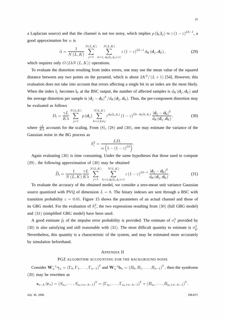
To evaluate the accuracy of the obtained model, we consider azero-mean unit variance Gaussian

source quantized with PVQ of dimensionL = 8. The binary indexes are sent through a BSC with

transition probabilityε = 0.01. Figure 15 shows the parameters of an actual channel and those of

its GBG model. For the evaluation ofσ2i , the two expressions resulting from(30) (full GBG model)

and (31) (simplified GBG model) have been used.

A good estimatepi of the impulse error probability is provided. The estimate of σ2i provided by

(30) is also satisfying and still reasonable with(31). The most difficult quantity to estimate isσ2g.

Nevertheless, this quantity is a characteristic of the system, and may be estimated more accurately

by simulation beforehand.

APPENDIX II

PGZ ALGORITHM ACCOUNTING FOR THE BACKGROUND NOISE

ConsiderW−1n γn = (Γ0,Γ1, . . . ,Γn−1)

T andW−1n bn = (B0, B1, . . . , Bn−1)

T , then the syndrome

(20) may be rewritten as

sn−k (rn) = (Sa0, . . . , Sa0+n−k−1)

T = (Γa0, . . . ,Γa0+n−k−1)

T + (Ba0, . . . , Ba0+n−k−1)

T .

July 30, 2006 DRAFT

26

0.5 1 1.5 2 2.50

0.2

0.4

0.6

0.8

R

actual channelGBG model

0.5 1 1.5 2 2.52

2.5

3

3.5

4

4.5

5

R

actual channelsimplified GBG modelfull GBG model

0.5 1 1.5 2 2.50

0.02

0.04

0.06

0.08

0.1

R

actual channelGBG model

0.5 1 1.5 2 2.56

8

10

12

14

16

18

R

actual channelsimplified GBG modelfull GBG model

pi

10lo

g(

)10

¾¾

ig

²²

/

¾g²

¾i²

Fig. 15. Comparison of a joint channel and its GBG model (L = 8 dimension PVQ followed by a BSC)

Assuming that there is no background gaussian noise, the classical PGZ algorithm would show

that λν has to satisfy

Γ∗n−k−ν,ν .λν = −Γ∗

n−k−ν,1 (32)

with Γn−k−ν,1 =(

Γa0+ν . . . Γa0+n−k−1

)Tand

Γn−k−ν,ν =

Γa0+ν−1 · · · Γa0

..... .

...

Γa0+n−k−2 · · · Γa0+n−k−1−ν

.

Assuming thatΓn−k−ν,ν andΓn−k−ν,1 are available,(32) may be solved in a least-squares sense

for λν

λν = −(ΓT

n−k−ν,ν.Γ∗n−k−ν,ν

)−1ΓT

n−k−ν,ν.Γ∗n−k−ν,1. (33)

In what follows, it is shown thatΓTn−k−ν,ν .Γ

∗n−k−ν,ν , Γn−k−ν,ν andΓn−k−ν,1 may be estimated

from the syndrome(20).

Let Bn−k−ν,1 =(

Ba0+ν . . . Ba0+n−k−1

)and

Bn−k−ν,ν =

Ba0+ν−1 · · · Ba0

.... . .

...

Ba0+n−k−2 · · · Ba0+n−k−1−ν

using the syndrome(20), Sn−k−ν,1 may be written as

Sn−k−ν,1 = Γn−k−ν,1 + Bn−k−ν,1 (34)

July 30, 2006 DRAFT

27

andSn−k−ν,ν as

Sn−k−ν,ν = Γn−k−ν,ν + Bn−k−ν,ν . (35)

Then

SHn−k−ν,νSn−k−ν,ν = ΓH

n−k−ν,νΓn−k−ν,ν + ΓHn−k−ν,νBn−k−ν,ν

+BHn−k−ν,νΓn−k−ν,ν + BH

n−k−ν,νBn−k−ν,ν . (36)

Impulse and Gaussian background noise are uncorrelated, thus E(ΓH

n−k−ν,νBn−k−ν,ν

)= 0ν and

E(BH

n−k−ν,νΓn−k−ν,ν

)= 0ν . Moreover, one may easily verify thatE (Bn−k−ν,1) = 0n−k−ν,1,

E (Bn−k−ν,ν) = 0n−k−ν,ν , andE(BH

n−k−ν,νBn−k−ν,ν

)= n−k−ν

n σ2gIν .

ML estimates forΓn−k−ν,ν and Γn−k−ν,1 may then be obtained asΓn−k−ν,ν = Sn−k−ν,ν and

Γn−k−ν,1 = Sn−k−ν,1. Using (36) and the two previous estimates, one may deduce an estimate for

ΓHn−k−ν,ν .Γn−k−ν,ν , as

ΓHn−k−ν,ν .Γn−k−ν,ν = SH

n−k−ν,νSn−k−ν,ν − (n − k − ν)

nσ2

gIν .

The three previous estimates may then be used in(33) to get (22) .

APPENDIX III

PDF OF THE NORM OF THE SYNDROME

The aim of this appendix is to derive a probability distribution of the norm of the syndrome under

the assumption thatν errors have corrupted the transmitted codeword.

Considering the vector of impulsesγ(ρ(ν)

)=(γρ(ν)

1, . . . , γρ(ν)

ν

)T, (20) may be rewritten as

sn−k

(ρ(ν)

)= Vn−k,ν

(ρ(ν)

)γ(ρ(ν)

)+ Rn−k,nW

−1n bn, (37)

with Vn−k,ν

(ρ(ν)

)= Rn−k,n

(wT

bρ1. . . wT

bρν

)T, see Section III-C.3. Then,

sn−k

(ρ(ν)

)=(

Vn−k,ν

(ρ(ν)

)Rn−k,nW

−1n

) γ

(ρ(ν)

)

bn

is a linear combination of gaussian variables with differing variances. Consider

∆ν+n (ν) = diag

(1/σi , . . . , 1/σ i

ν times, 1/σg, . . . , 1/σg

n times

),

thensn−k

(ρ(ν)

)= Q

(ρ(ν)

)zν+n, with

Q(ρ(ν)

)=(

Vn−k,ν

(ρ(ν)

)Rn−k,nW

−1n

)∆−1

ν+n (ν)

and

zν+n = ∆ν+n (ν)

γ

(ρ(ν)

)

bn

July 30, 2006 DRAFT

28

is a gaussian vector with iid unit variance entries.

The matrixQH(ρ(ν)

)Q(ρ(ν)

)is hermitian symmetric and thus may be diagonalized as

QH(ρ(ν)

)Q(ρ(ν)

)= KH

(ρ(ν)

)G(ρ(ν)

)K(ρ(ν)

),

with K(ρ(ν)

)unitary and real andG

(ρ(ν)

)diagonal. The norm of the syndrome may then be written

as

y(ρ(ν)

)= sH

n−k

(ρ(ν)

)sn−k

(ρ(ν)

)=(K(ρ(ν)

)zν+n

)HG(ρ(ν)

)K(ρ(ν)

)zν+n.

As zν+n is normal with unit variance,K(ρ(ν)

)zν+n is also normal with unit variance. Thus,

y(ρ(ν)

)=

rank(Q(ρ(ν)))∑

k=1

g2k

(ρ(ν)

)|zk|2 ,

wheregk

(ρ(ν)

)are the diagonal entries ofG

(ρ(ν)

). As rank

(Q(ρ(ν)

))= n − k, the probability

distribution ofy(ρ(ν)

)is the convolution of scaledχ2 distributions with one degree of freedom

p(y|ρ(ν), ν

)=

n−k⊗

k=1

χ21

(gk

(ρ(ν)

), y)

, (38)

with χ21 (gk, y) = 1√

2g2kΓ(1/2)

(y/g2

k

)−1/2exp

(−y/

(2g2

k

))and may be evaluated using [55].

The pdf of the syndrome under the hypothesis that there areν impulse errors is obtained by

averaging(38) over all possible values ofρ(ν)

p (y|ν) =∑

ρ(ν)

p(y|ρ(ν), ν

)p(ρ(ν)|ν

). (39)

REFERENCES

[1] A. Gabay, P. Duhamel, and O. Rioul, “Real BCH codes as joint source channel code for satellite images coding,” in

Proc. Globecom, San Francisco, USA, nov 2000, pp. 820–824.

[2] A. Gabay, O. Rioul, and P. Duhamel, “Joint source-channel coding using structured oversampled filters banks applied

to image transmission,” inProc. ICASSP, 2001, pp. 2581–2584.

[3] F. Abdelkefi, F. Alberge, and P. Duhamel, “A posteriori control of complex Reed Solomon decoding with application

to impulse noise cancellation in hiperlan2,” inProc. ICC, 2002, pp. 659 – 663.

[4] ——, “Impulse noise correction in hiperlan 2: Improvement of the decoding algorithm and application to PAPR

reduction,” inProceedings of ICC, 2003, pp. 2094 – 2098.

[5] C. E. Shannon, “A mathematical thoery of communication,” Bell Syst. Tech. J., 1948.

[6] S. B. Zahir Azami, P. Duhamel, and O. Rioul, “Joint sourcechannel coding : Panorama of methods,”Proceedings of

CNES workshop on Data Compression, Nov. 1996.

[7] K. Sayood,Introduction to Data Compression, Second Edition. San Francisco: Morgan Kaufmann, 2000.

[8] K. Ramchandran, A. Ortega, K. M. Uz, and M. Vetterli, “Multiresolution broadcast for HDTV using joint

source/Channel coding,”IEEE Tansactions on SAC, vol. 11, pp. 3–14, 1993.

[9] J. Hagenauer, “Rate-compatible punctured convolutional codes (RCPC codes) and their applications,”IEEE Trans.

Communications, vol. 36, no. 4, pp. 389–400, 1988.

[10] I. Kozintsev and K. Ramchandran, “Robust image transmission over energy-constrained time-varying channels using

multiresolution joint source-channel coding,”IEEE trans. Signal Processing, vol. 46, no. 4, pp. 1012–1026, 1998.

July 30, 2006 DRAFT

29

[11] N. Farvardin and V. Vaishampayan, “Optimal quantizer design for noisy channels: An approach to combined source-

channel coding,”IEEE Transactions on Information Theory, vol. 33, no. 6, pp. 827–837, 1991.

[12] Y. Zhou and W. Y. Chan, “Multiple description quantizerdesign using a channel optimized quantizer approach,” in

Proceedings of the 38th Annual Conference on Information Sciences and Systems (CISS’04), 2004.

[13] Y. Takishima, M. Wada, and H. Murakami, “Reversible variable length codes,”IEEE Trans. Commun, vol. 43, no.

2-4, pp. 158–162, 1995.

[14] K. Lakovic and J. Villasenor, “On design of error-correcting reversible variable length codes,”IEEE Communications

Letters, vol. 6, no. 8, pp. 337– 339, 2002.

[15] J. Wang, L.-L. Yang, and L. Hanzo, “Iterative construction of reversible variable-length codes and variable-length

error-correcting codes,”IEEE Communications Letters, vol. 8, no. 11, pp. 671– 673, 2004.

[16] J. Hagenauer, “Source-controlled channel decoding,”IEEE trans. on Communications, vol. 43, no. 9, pp. 2449–2457,

1995.

[17] V. Buttigieg and P. Farrell, “A MAP decoding algorithm for variable-length error-correcting codes,” inCodes and

Cyphers: Cryptography and Coding IV. Essex, England: The Inst. of Mathematics and its Appl., 1995, pp. 103–119.

[18] R. Bauer and J. Hagenauer, “Symbol-by-symbol MAP decoding of variable length codes,” inProc. 3rd ITG Conference

Source and Channel Coding, Munchen, 2000, pp. 111–116.

[19] K. Sayood, H. H. Otu, and N. Demir, “Joint source/channel coding for variable length codes,”IEEE Trans. Commun.,

vol. 48, pp. 787–794, 2000.

[20] R. Thobanen and J. Kliewer, “Robust decoding of variable-length encoded Markov sources using a three-dimensional

trellis,” IEEE Communications Letters, vol. 7, no. 7, pp. 320–322, 2003.

[21] P. Burlina and F. Alajaji, “An error resilient scheme for image transmission over noisy channels with memory,”IEEE

trans. on Image Processing, vol. 7, no. 4, pp. 593–600, 1998.

[22] J. Garcia-Frıas and J. D. Villasenor, “Joint turbo decoding and estimation of hidden Markov sources,”IEEE J. Selected

Areas in Communications, vol. 19, no. 9, pp. 1671–1679, 2001.

[23] J. Garcia-Frias and Y. Zhao, “Compression of binary memoryless sources using punctured turbo codes,”IEEE

Communications Letters, vol. 6, no. 9, pp. 394 – 396, 2002.

[24] J. Hagenauer, N. Dutsch, J. Barros, and A. Schaefer, “Incremental and decremental redundancy in turbo source–channel

coding,” in Proc. Int. Symposium on Control, Communications and SignalProcessing, March 2004, pp. 595–598.

[25] J. Hagenauer, J. Barros, and A. Schaefer, “Lossless turbo source coding with decremental redundancy,” inProc. 5th

Int. ITG Conference on Source and Channel Coding, January 2004, pp. 333–339.

[26] F. Hekland, G. E. Øien, and T. A. Ramstad, “Using 2: 1 shannon mapping for joint source-channel coding,” inProc.

DCC, 2005, pp. 223–232.

[27] C. E. Shannon, “Communication in the presence of noise,” Proc. IRE, vol. 37, pp. 10–21, 1949.

[28] J. K. Wolf, “Redundancy, the discrete Fourier transform, and impulse noise cancellation,”IEEE Transactions on

Communications, vol. 31, no. 3, pp. 458–461, 1983.

[29] T. G. Marshall, “Coding of real-number sequences for error correction: A digital signal processing problem,”IEEE

Journal on Selected Areas in Communications, vol. 2, no. 2, pp. 381–392, 1984.

[30] J. L. Wu and J. Shiu, “Discrete cosine transform in errorcontrol coding,”IEEE trans. on Communications, vol. 43,

no. 5, pp. 1857–1861, 1995.

[31] R. E. Blahut,Theory and Practice of Error Control Codes. Reading, MA: Addison-Wesley, 1984.

[32] F. Marvasti, M. Hasan, M. Echhart, and S. Talebi, “Efficient algorithms for burst error recovery using FFT and other

transform kernels,”IEEE trans. on Signal Processing, vol. 47, no. 4, pp. 1065–1075, 1999.

[33] G. R. Redinbo, “Decoding real block codes: Activity detection, wiener estimation,”IEEE trans. on Information Theory,

vol. 46, no. 2, pp. 609–623, 2000.

July 30, 2006 DRAFT

30

[34] M. Ghosh, “Analysis of the effect of impulse noise on multicarrier and single carrier QAM systems,”IEEE Transactions

on Communication, vol. 44, no. 2, pp. 145–147, 1996.

[35] O. Rioul, “A spectral algorithm for removing salt and pepper from images,” inProc. IEEE Digital Signal Processing

Workshop. 3, 1996, pp. 275–278.

[36] G. Rath and C. Guillemot, “Performance analysis and recursive syndrome decoding of DFT codes for bursty erasure

recovery,” IEEE trans. on Signal Processing, vol. 51, no. 5, pp. 1335–1350, 2003.

[37] ——, “Frame-theoretic analysis of DFT codes with erasures,” IEEE trans. on Signal Processing, vol. 52, no. 2, pp.

447–460, 2004.

[38] R. E. Totty and G. C. Clark, “Reconstruction error in waveform transmission,”IEEE Transactions on Information

Theory, vol. 13, no. 2, pp. 336–338, 1967.

[39] A. J. Kurtenbach and P. A. Wintz, “Quantizing for noisy channels,”IEEE Trans. Communication Technology, vol. 17,

no. 10, pp. 292–302, 1969.

[40] J. B. Anderson,Digital Transmission Ingineering, 2nd ed. Wiley, 2005.

[41] R. E. Blahut, “Computation of channel capacity and rate-distorsion functions,”IEEE transactions on Information

Theory, vol. 18, no. 4, pp. 460–473, 1972.

[42] M. Barkat,Signal, Detection and Estimation. Norwood, MA: Artech House, 1991.

[43] P. J. S. G. Ferreira, D. M. S. Santos, and V. M. A. Afreixo,“New results and open problems in real-number codes,”

in Proceedings of EUSIPCO, 2004.

[44] P. Duhamel and M. Vetterli, “Fast Fourier transforms: Atutorial review and a state of the art,”Signal Processing,

vol. 19, no. 4, pp. 259–299, 1990.

[45] Y. Shoam and A. Gersho, “Efficient bit allocation for an arbitrary set of quantizers,”IEEE Trans. on Acoustics, Speech,

and Signal Processing, vol. 36, no. 9, pp. 1445–1453, 1988.

[46] “CNES report WGISS-8,” 1999,http://www.space.qinetiq.com/ceos/docs/cnes report wgiss.doc.

[47] C. Lambert-Nebout, C.Latry, G. Moury, C. Parisot, M. Antonini, and M. Barlaud, “On-board optical image compression

for future high resolution remote sensing systems,” inProceedings of SPIE2000, vol. 4115, San Diego, USA, 2000.

[48] A. K. Jain, Fundamentals of Digital Image Processing. Englewood Cliffs, NJ: Prentice-Hall, 1989.

[49] http://smsc.cnes.fr/PLEIADES/.

[50] J. Kliewer and A. Mertins, “Soft-input reconstructionof binary transmitted quantized overcomplete expansions,” IEEE

Signal Processing Letters, vol. 11, no. 11, pp. 899–903, 2004.

[51] S. Marinkovic and C. Guillemot, “Joint source-channelcoding by means of oversampled filter banks codes,”Eurasip

journal on applied signal processing, no. 4, pp. 510–524, 2005.

[52] F. Labeau, J. Chiang, M. Kieffer, P. Duhamel, L. Vandendorpe, and B. Mack, “Oversampled filter banks as error

correcting codes: theory and impulse correction,”IEEE Trans. on Signal Processing, vol. 53, no. 12, pp. 4619 – 4630,

2005.

[53] T. R. Fischer, “A pyramid vector quantization,”IEEE Trans. Inform. Theory, vol. 32, pp. 568–583, 1986.

[54] A. C. Hung, E. K. Tsern, and T. H. Meng, “Error-resilientpyramid vector quantization for image compression,”IEEE

Trans. Image Processing, vol. 7, no. 10, pp. 1373–1386, 1998.

[55] R. B. Davies, “The distribution of a linear combinationof χ2 random variables,”Statistical algorithms, vol. 29, pp.

323–333, 1980.

July 30, 2006 DRAFT